Article

Dynamic Analysis of a Delayed Differential Equation for Ips subelongatus Motschulsky-Larix spp.

Department of Mathematics, Northeast Forestry University, Harbin 150040, China
*
Author to whom correspondence should be addressed.
Axioms 2024, 13(4), 232; https://doi.org/10.3390/axioms13040232
Submission received: 28 February 2024 / Revised: 26 March 2024 / Accepted: 30 March 2024 / Published: 1 April 2024
(This article belongs to the Special Issue Dynamical Systems: Theory and Applications in Mathematical Biology)

Abstract

:
The protection of forests and the mitigation of pest damage to trees play a crucial role in mitigating the greenhouse effect. In this paper, we first establish a delayed differential equation model for Ips subelongatus Motschulsky-Larix spp., where the delay parameter represents the time required for trees to undergo curing. Second, we analyze the stability of the equilibrium of the model and derive the normal form of Hopf bifurcation using a multiple-time-scales method. Then, we analyze the stability and direction of Hopf bifurcating periodic solutions. Finally, we conduct simulations to analyze the changing trends in pest and tree populations. Additionally, we investigate the impact of altering the rate of artificial planting on the system and provide corresponding biological explanations.

1. Introduction

At present, the issue of the greenhouse effect has received widespread attention worldwide. Human activities release a significant amount of greenhouse gases, with CO2 being the most crucial among them, as it increasingly traps solar heat and warms the global climate. Forests have been identified as a major leverage for climate change mitigation because of their capacity to fix atmospheric CO2 and transform it into organic carbon, in biomass and then in soils [1]. However, tree damage and death associated with insect and disease disturbance can reduce this carbon sequestration capacity [2]. Solving the problem of forest diseases and pests could also help mitigate the greenhouse effect. Scholars have conducted corresponding research on forest diseases and pests. Some scholars proposed the use of microorganisms and fungi for pest control [3,4,5]. Some scholars used modern technologies such as drones and remote sensing to monitor forests by constructing models [6,7,8]. Some scholars introduced methods for suppressing pest outbreaks by establishing mathematical models. For example, Jentsch et al. [9] used a difference equation model for the age structure of bark beetle outbreaks and forest fires, indicating that fires can not only remove infected trees but also alter their structure, thereby suppressing pest outbreaks. Xu et al. [10] described the process of controlling pests through pulse spraying of pesticides within a given time by constructing a dynamic system of logistic differential equations with pulse effects. It solved the problem of pest control within a limited time.
To address the issue of forest pests and diseases, an important approach in the field of mathematics is to establish mathematical models for simulating these problems. Various models of forest diseases and pests have been studied [11,12,13]. Many scholars provided a theoretical analysis of the models from an equation analysis perspective [14,15,16,17,18]. For example, Song et al. [14] considered a diffusive predator–prey system with memory-based diffusion and Holling type-II functional response. Jiang et al. [15] derived the normal form up to the third order for the Turing–Hopf bifurcation.
China’s total forest area ranks fifth in the world. The Northeast Forest Region is the largest natural forest region in China. Larix spp. is one of the most important trees in the northeast forest area. Therefore, giving attention to Larix spp. resources has a huge impact on China’s forests and the world’s forest resources. Some scholars have conducted research on the genes and genetics of Larix spp. [19,20]. Some scholars have studied the factors that hinder the growth and development of larch trees. For example, Skrzecz et al. [21] found that larch receded strongly in forested agricultural lands due to tillage techniques used before planting that prevented proper root development of larch seedlings and the severe impact of the large larch bark beetle (Heer). Chen et al. [22] showed that Ips subelongatus Motschulsky is a serious pest of northeastern larch that can kill relatively healthy trees during outbreak periods.
Ips subelongatus (Motschulsky) is an Asian larch bark beetle that causes significant damage to several species of larch in East Asia, particularly in northern China [23], such as the Da Hinggan and Xiao Hinggan ranges in the Inner Mongolia autonomous region and Heilongjiang Province, south-eastern Heilongjiang and the Changbai Mountains in Liaoning Province, and middle Inner Mongolia autonomous region, consequently threatening local plantations [24]. Ips subelongatus exhibits a high reproductive rate and low mortality rate in environments with high humidity. The larvae feed on phloem from both sides of the main tunnel, while the sub-tunnel gradually widens and lengthens as they grow. Upon reaching adulthood, the larvae emerge through small holes and disperse to find new hosts, establishing fresh tunnels. In addition, the weaker the vitality of trees and the fresher the fallen trees, the more rampant the pests. The smaller the canopy density of forest, the more severe the damage to the tree. Figure 1 shows the infection mechanism of Ips subelongatus Motschulsky.
Currently, scholars have conducted extensive research on the occurrence pattern, biological characteristics, and genetic modification of Ips subelongatus Motschulsky [25,26,27,28]. However, there have been few studies on the use of mathematical models to study Ips subelongatus Motschulsky. The research motivation for this article was as follows: by establishing a delayed differential equation, where the delay represents the time required for infected trees to regain their health, we discuss strategies for maintaining forest stability in the face of Ips subelongatus Motschulsky.
The rest of this article is arranged as follows: In Section 2, a delayed differential equation is established based on the living habits and infection ability of the Ips subelongatus Motschulsky. In Section 3, we analyze the existence and stability of the nonnegative equilibrium point, as well as the existence of Hopf bifurcation. In Section 4, we calculate the normal form of Hopf bifurcation. In Section 5, we use numerical simulations to verify the correctness of the results. In Section 6, we provide some conclusions.

2. Mathematical Modeling

In this section, we establish the following model:
d X d t = r X ( 1 X N ) β 1 X M X , d S d t = γ I ( t τ ) k β 2 I X S + R , d I d t = k β 2 I X S γ I ( t τ ) β 2 I ,
where r, N, β 1 , M, γ , k, β 2 , and R are nonnegative parameters. The specific meanings of variables and parameters can be seen in Table 1.
Next, we offer some explanations about the system (1).
(a)
Based on the biological characteristics of Ips subelongatus Motschulsky, we denote X ( t ) as the population size of Ips subelongatus Motschulsky. The reproductive capacity of pests is subject to resource constraints, resulting in a gradual decrease in their growth rate as they approach the environmental capacity N, we assume that the growth rate of pests follows the logistic model; that is, r X ( 1 X N ) . Moreover, the mortality rate pests experience not only depends on their own mortality rate β 1 , but also depends on predation by natural predators M. Based on this analysis, we establish the first equation of system (1) to describe the rate of change in the pest population.
(b)
We assume that susceptible Larix spp. S ( t ) becomes infected Larix spp. I ( t ) after being infected by pests. Infected Larix spp. I ( t ) can be cured and transformed back into susceptible Larix spp. S ( t ) . The process of curing requires a certain amount of time, taking into account practical considerations; thus, we introduce τ as the curing duration. The rate at which cured infected trees change is denoted as γ I ( t τ ) .
(c)
In the conventional infectious disease model, the infection rate is constant, but the infection ability of Ips subelongatus Motschulsky is stronger when the canopy density of the trees is lower, indicating that pests have a stronger ability to infect as more trees die. Therefore, we establish an infection rate function f ( β 2 I ) = k β 2 I , where k represents the infection rate coefficient and β 2 I represents the rate of change in infected trees that have died. This function reflects that the infection rate is directly proportional to β 2 I . At this point, the infectiousness of the pest is denoted k β 2 I X . Thus, the transmission rate from susceptible trees S ( t ) to infected trees I ( t ) can be denoted k β 2 I X S . Since the forest is not isolated, new Larix spp. trees will be planted at a certain rate R. Based on the above analysis, we can establish a relationship between susceptible and infected trees.
Remark 1.
As for system (1), several scholars have also conducted research on similar models, such as the infectious disease model. Majee et al. [29] assumed a constant infection rate, while we assume the infection rate as a function considering the biological characteristics of Ips subelongatus. Additionally, Majee et al. treated the cure rate as a saturation function, while we treat it as a constant. Li et al. [30] considered the infection rate to be a saturation function, whereas we regard it as directly proportional.

3. Stability Analysis of Equilibrium and Existence of Hopf Bifurcation

In this section, we discuss the system (1). We sequentially analyze the existence and stability of the equilibrium point, as well as the existence of Hopf bifurcation.

3.1. The Existence of Equilibrium

We make the following assumption:
( A 1 ) r > β 1 + M .
Remark 2.
r represents the proliferation rate of pests, β 1 represents the natural mortality rate of pests, and M represents the mortality rate caused by pests being preyed upon by natural enemies. Assumption (A1) implies that the proliferation rate of the pest exceeds its mortality rate. This is a universal law of nature, because if a population wants to exist, it must meet this condition, otherwise, extinction is inevitable.
When ( A 1 ) holds, we can obtain the unique and positive equilibrium of system (1):
E * = ( X * , S * , I * ) ,
where X * = N ( r β 1 M ) r , S * = γ + β 2 k β 2 X * , I * = R β 2 .

3.2. The Stability of Equilibrium and Existence of Hopf Bifurcation

For the convenience of the subsequent discussion, we denote a = k R X * = k R N ( r β 1 M ) r > 0 under ( A 1 ) .
We can obtain the characteristic equation of the system (1) at equilibrium E * , as follows:
( λ β 1 M + r ) [ λ 2 + ( γ e λ τ γ + a ) λ + a β 2 ] = 0 .
When τ = 0 , the characteristic Equation (2) becomes
( λ β 1 M + r ) ( λ 2 + a λ + a β 2 ) = 0 .
Under the assumption ( A 1 ) , we can clearly see from Vieta theorem that the Equation (3) has three roots with negative real parts. The equilibrium E * of the system (1) with τ = 0 is locally asymptotically stable.
Next, we discuss the existence of Hopf bifurcating periodic solutions near equilibrium E * when τ > 0 . Under the assumption ( A 1 ) , we can see that Equation (2) always has a root with a negative real part:
λ 1 = β 1 + M r .
Thus, we only need to consider the following equation:
λ 2 + ( γ e λ τ γ + a ) λ + a β 2 = 0 .
Lemma 1.
When ( a 2 2 a γ 2 a β 2 ) 2 4 a 2 β 2 2 > 0 and a 2 2 a γ 2 a β 2 < 0 , Equation (4) has a pair of pure imaginary roots ± i ω .
Proof. 
We introduce λ = i ω into Equation (4), then separate the real and imaginary parts, and finally obtain the following equations:
ω 2 + ω γ sin ( ω τ ) + a β 2 = 0 , ω γ cos ( ω τ ) ω γ + a ω = 0 .
Thus, we have
sin ( ω τ ) = ω 2 a β 2 γ ω , cos ( ω τ ) = γ a γ .
Let z = ω 2 , we obtain
h ( z ) = z 2 + ( a 2 2 a γ 2 a β 2 ) z + a 2 β 2 2 = 0 .
When ( a 2 2 a γ 2 a β 2 ) 2 4 a 2 β 2 2 < 0 , Equation (6) has no real root. When ( a 2 2 a γ 2 a β 2 ) 2 4 a 2 β 2 2 > 0 , Equation (6) has two distinct real roots:
z 1 , 2 = ( a 2 2 a γ 2 a β 2 ) ( a 2 2 a γ 2 a β 2 ) 2 4 a 2 β 2 2 2 , z 1 , 2 < 0 , when a 2 2 a γ 2 a β 2 > 0 . z 1 , 2 > 0 , when a 2 2 a γ 2 a β 2 < 0 .
Thus, when ( a 2 2 a γ 2 a β 2 ) 2 4 a 2 β 2 2 > 0 and a 2 2 a γ 2 a β 2 < 0 , z 1 , 2 > 0 , ω is a real number, Equation (4) has a pair of pure imaginary roots ± i ω . □
Assume that Equation (6) has two roots z 2 > z 1 > 0 , and h ( z 1 ) < 0 , h ( z 2 ) > 0 . Then, by substituting ω k = z k ( k = 1 , 2 ) into the Equation (5), we obtain the expression for τ :
τ k ( j ) = 1 ω k [ arccos ( P k ) + 2 j π ] , Q k 0 , 1 ω k [ 2 π arccos ( P k ) + 2 j π ] , Q k < 0 . k = 1 , 2 , j = 0 , 1 , 2 , .
where
Q k = sin ( ω k τ k ( j ) ) = ω k 2 a β 2 ω k γ , P k = cos ( ω k τ k ( j ) ) = γ a γ .
Lemma 2.
Under the assumption ( A 1 ) , system (1) satisfies the transversal condition for generating Hopf bifurcation; that is,
Re ( d λ d τ ) | τ k ( j ) = γ 2 ω 2 h ( z ) 0 , k = 1 , 2 , j = 0 , 1 , 2 , .
Proof. 
Take the derivative of λ on both sides of Equation (4).
We have
( 2 λ + γ e λ τ τ λ γ e λ τ γ + a ) d λ = γ λ 2 e λ τ d τ .
d τ d λ = 2 λ + γ e λ τ τ λ γ e λ τ γ + a γ λ 2 e λ τ = 2 λ + γ e λ τ γ + a γ λ 2 e λ τ τ λ .
Because when τ = τ k ( j ) , τ λ is purely imaginary, k = 1 , 2 , j = 0 , 1 , 2 . Thus,
R e ( d τ d λ ) | τ k ( j ) = R e ( 2 λ + γ e λ τ γ + a γ λ 2 e λ τ ) | τ k ( j ) = R e [ ( a γ ) c o s ( ω τ ) 2 ω s i n ( ω τ ) + γ γ ω 2 ] | τ k ( j ) .
According to Equation (5), we obtain
R e ( d τ d λ ) | τ k ( j ) = R e ( 2 ω 2 + a 2 2 a γ 2 a β 2 γ 2 ω 2 ) | τ k ( j ) = h ( z ) γ 2 ω 2 .
When z 2 > z 1 > 0 , h ( z 1 ) < 0 , h ( z 2 ) > 0 . Thus,
Re ( d λ d τ ) | τ k ( j ) = γ 2 ω 2 h ( z ) 0 , k = 1 , 2 , j = 0 , 1 , 2 , .
Based on the above, we obtain the following conclusions:
Theorem 1.
When (A1) holds, considering system (1), we draw the following conclusions:
(i)
If ( a 2 2 a γ 2 a β 2 ) 2 4 a 2 β 2 2 < 0 or ( a 2 2 a γ 2 a β 2 ) 2 4 a 2 β 2 2 > 0 , a 2 2 a γ 2 a β 2 > 0 , the equilibrium E * is locally asymptotically stable when τ 0 .
(ii)
If ( a 2 2 a γ 2 a β 2 ) 2 4 a 2 β 2 2 > 0 and a 2 2 a γ 2 a β 2 < 0 , the Equation (6) has two roots z 2 > z 1 > 0 , and h ( z 1 ) < 0 , h ( z 2 ) > 0 . Then, n N make 0 < τ 2 ( 0 ) < τ 1 ( 0 ) < τ 2 ( 1 ) < τ 1 ( 1 ) < < τ 1 ( n 1 ) < τ 2 ( n ) < τ 2 ( n + 1 ) < . When τ [ 0 , τ 2 ( 0 ) ) l = 1 n ( τ 1 ( l 1 ) , τ 2 ( l ) ) , the equilibrium E * of the system (1) is locally asymptotically stable. And when τ l = 0 n 1 ( τ 2 ( l ) , τ 1 ( l ) ) ( τ 2 ( n ) , + ) , the equilibrium E * is unstable, where τ k ( j ) ( k = 1 , 2 , j = 0 , 1 , 2 ) is given in Equation (7).

4. Normal Form of Hopf Bifurcation

In this section, we derive the normal form of the Hopf bifurcation of the system (1) using the multiple-time-scales method. In order to reflect the actual situation, we study the delay required for curing trees and the impact of this delay. We consider the time-delay τ as a bifurcation parameter. We make τ = τ c + ε μ , where τ c = τ k ( j ) is given in the Equation (7), which is the Hopf bifurcation critical value, ε is the dimensionless scale parameter, and μ is the perturbation parameter. When τ = τ k ( j ) , Equation (4) has the eigenvalue λ = i ω , and the system (1) undergoes a Hopf bifurcation at equilibrium E * . Then, we transform the equilibrium E * to the origin and change the time scale; that is, let t t τ . Finally, we obtain the following form:
Z ˙ = τ A Z ( t ) + τ B Z ( t 1 ) + τ F ( Z ( t ) , Z ( t 1 ) ) ,
where
Z ( t ) = ( X ( t ) , S ( t ) , I ( t ) ) T , Z ( t 1 ) = ( X ( t 1 ) , S ( t 1 ) , I ( t 1 ) ) T , F ( Z ( t ) , Z ( t 1 ) ) = ( r X 2 N , k β 2 ( I X S + S * I X + X * I S + I * X S ) , k β 2 ( I X S + S * I X + X * I S + I * X S ) ) T ,
and
A = r 2 r X * N β 1 M 0 0 k β 2 S * I * k β 2 X * I * k β 2 S * X * k β 2 I * S * k β 2 I * X * k β 2 S * X * β 2 ,   B = 0 0 0 0 0 γ 0 0 γ .
We set h as the eigenvector corresponding to the eigenvalue λ = i ω τ of the linear system of Equation (8), and h * as the eigenvector corresponding to the eigenvalue λ = i ω τ of the adjoint matrix of the linear system of Equation (8), and satisfy the following conditions:
h * , h = h * ¯ T h = 1 .
Through calculation, we obtain that
h = ( 0 , b , 1 ) T , h * = d ( p , 1 , c ) T ,
where
b = 1 β 2 i ω , c = 1 ω i a , p = ω R i [ k R β 2 ( x * ) 2 ] ( i w + β 1 + M r ) , d = 1 b ¯ + c .
We assume that the solution of the Equation (8) is in the following form:
Z ( t ) = Z ( T 0 , T 1 , T 2 ) = k = 1 + ε k Z k ( T 0 , T 1 , T 2 ) ,
where
Z ( T 0 , T 1 , T 2 , ) = ( X ( T 0 , T 1 , T 2 , ) , S ( T 0 , T 1 , T 2 , ) , I ( T 0 , T 1 , T 2 , ) ) T , Z k ( T 0 , T 1 , T 2 , ) = ( X k ( T 0 , T 1 , T 2 , ) , S k ( T 0 , T 1 , T 2 , ) , I k ( T 0 , T 1 , T 2 , ) ) T .
The derivative of t is transformed into
d d t = T 0 + ε T 1 + ε 2 T 2 + = D 0 + ε D 1 + ε 2 D 2 + ,
where D i is a differential operator, and
D i = T i , ( i = 0 , 1 , 2 , ) .
we have
Z ˙ ( t ) = ε D 0 Z 1 + ε 2 D 1 Z 1 + ε 3 D 2 Z 1 + ε 2 D 0 Z 2 + ε 3 D 1 Z 2 + ε 3 D 0 Z 3 + .
By using Taylor expansion I ( T 0 1 , ε ( T 0 1 ) , ε 2 ( T 0 1 ) , ) at I ( T 0 1 , T 1 , T 2 , ) , we obtain
I ( t 1 ) = ε I 1 , τ c + ε 2 I 2 , τ c + ε 3 I 3 , τ c ε 2 D 1 I 1 , τ c ε 3 D 2 I 1 , τ c ε 3 D 1 I 2 , τ c + ,
where I j , τ c = I j ( T 0 1 , T 1 , T 2 , ) , j = 1 , 2 , .
By substituting the Equations (10)–(12) into Equation (8) and separating the coefficients of ε , ε 2 , and ε 3 , we obtain the following equations:
D 0 X 1 τ c r X 1 ( 1 2 X * N β 1 M ) = 0 , D 0 S 1 τ c [ γ I 1 , τ c k β 2 ( X * S * I 1 + I * S * X 1 + I * X * S 1 ) ] = 0 , D 0 I 1 τ c [ k β 2 ( X * S * I 1 + I * S * X 1 + I * X * S 1 ) γ I 1 , τ c β 2 I 1 ] = 0 .
D 0 X 2 τ c X 2 ( r 2 r X * N β 1 M ) = μ X 1 ( r 2 r X * N β 1 M ) τ c r N X 1 2 D 1 X 1 , D 0 S 2 γ τ c I 2 , τ c + τ c k β 2 ( X * I * S 2 + X * S * I 2 + S * I * X 2 ) = μ γ I 1 , τ c τ c γ D 1 I 1 , τ c τ c k β 2 ( S * I 1 X 1 + X * I 1 S 1 + I * X 1 S 1 ) μ k β 2 ( S * I * X 1 + X * I * S 1 + X * S * I 1 ) D 1 S 1 , D 0 I 2 τ c k β 2 ( X * S * I 2 + X * I * S 2 + I * S * X 2 ) + γ τ c I 2 , τ c + τ c β 2 I 2 = τ c k β 2 ( S * I 1 X 1 + X * I 1 S 1 + I * X 1 S 1 ) + μ k β 2 ( S * I * X 1 + X * I * S 1 + X * S * I 1 ) μ γ I 1 , τ c + τ c γ D 1 I 1 , τ c μ β 2 I 1 D 1 I 1 .
D 0 X 3 τ c ( r 2 X * r N β 1 M ) X 3 = μ ( r 2 X * r N β 1 M ) X 2 μ r N X 1 2 2 τ c r N X 1 X 2 D 2 X 1 D 1 X 2 , D 0 S 3 + k β 2 τ c ( I * S * X 3 + X * S * I 3 + I * X * S 3 ) γ τ c I 3 , τ c = τ c k β 2 [ S * ( I 1 X 2 + I 2 X 1 ) + X * ( I 1 S 2 + I 2 S 1 ) + I * ( X 1 S 2 + X 2 S 1 ) ] μ k β 2 ( S * I 1 X 1 + I * S 1 X 1 + X * S 1 I 1 + X * S * I 2 + I * S * X 2 + I * X * S 2 ) ) k β 2 τ c I 1 X 1 S 1 D 2 S 1 D 1 S 2 τ c γ ( D 2 I 1 , τ c D 1 I 2 , τ c ) + μ γ ( I 2 , τ c D 1 I 1 , τ c ) , D 0 I 3 k β 2 τ c ( I * S * X 3 + X * S * I 3 + I * X * S 3 ) + γ τ c I 3 , τ c + τ c β 2 I 3 = τ c k β 2 [ S * ( I 1 X 2 + I 2 X 1 ) + X * ( I 1 S 2 + I 2 S 1 ) + I * ( X 1 S 2 + X 2 S 1 ) ] + μ k β 2 ( S * I 1 X 1 + I * S 1 X 1 + X * S 1 I 1 + X * S * I 2 + I * S * X 2 + I * X * S 2 ) + k β 2 τ c I 1 X 1 S 1 μ β 2 I 2 D 2 I 1 D 1 I 2 μ γ ( I 2 , τ c D 1 I 1 , τ c ) + τ c γ ( D 2 I 1 , τ c D 1 I 2 , τ c ) .
The form of the solution to Equation (13) is as follows:
Z 1 = G h e i ω τ c T 0 + G ¯ h ¯ e i ω τ c T 0 ,
where h is given by Equation (9). We substitute solution (16) into the right part of Equation (14), denote the coefficient of e i ω τ c T 0 as m 1 , and then use h * , m 1 = 0 to obtain the expression of G T 1 as follows:
G T 1 = K μ G ,
where
K = v [ e i ω τ c γ k β 2 ( X * I * b + X * S * ) e i ω τ c γ c ¯ + k β 2 c ¯ ( X * I * b + X * S * ) β 2 c ¯ ] ,
with
v = ( e i ω τ c τ c γ + b e i ω τ c τ c γ c ¯ + c ¯ ) 1 .
Because μ represents a very small disturbance, it has little impact on higher-order terms. So, we ignore the parts of high-order terms with μ . We assume that the form of the solution to Equation (14) is as follows:
X 2 = g 0 e 2 i ω τ c T 0 + g ¯ 0 e 2 i ω τ c T 0 + l 0 , S 2 = g 1 e 2 i ω τ c T 0 + g ¯ 1 e 2 i ω τ c T 0 + l 1 , I 2 = g 2 e 2 i ω τ c T 0 + g ¯ 2 e 2 i ω τ c T 0 + l 2 ,
where
g 0 = 0 , g 2 = k β 2 X * G 2 b 2 i ω + β 2 + γ e 2 i ω τ c k β 2 X * [ I * ( 1 + β 2 i 2 ω ) + S * ] , g 1 = ( 1 + β 2 2 ω i ) g 2 , l 0 = 0 , l 1 = ( b + b ¯ ) G G ¯ I * , l 2 = 0 .
Then, we substitute solution (18) into the right part of Equation (15), denote the coefficient of e i ω τ c T 0 as m 2 , and then use h * , m 2 = 0 to obtain the expression of G T 2 , as follows:
G T 2 = H G 2 G ¯ ,
where
H = v τ c k β 2 X * ( 1 c ¯ ) ( b + b ¯ ) I * ,
where v is given in Equation (17).
Then, we obtain the normal form of the Hopf bifurcation of system (1) truncated by the cubic-order terms:
G ˙ = K μ G + H G 2 G ¯ ,
where K and H are given in Equations (17) and (19), respectively. We replace the polar coordinates in Equation (20) with G = ρ e i θ , and then obtain the normal form of Hopf bifurcation in polar coordinates:
ρ ˙ = Re ( K ) μ ρ + Re ( H ) ρ 3 , θ ˙ = Im ( K ) μ + Im ( H ) ρ 2 .
According to the normal form of Hopf bifurcation in polar coordinates, we only need to consider the first equation in system (21). Thus, the following theorem holds:
Theorem 2.
When Re ( K ) μ Re ( H ) < 0 , there is an equilibrium point r * = Re ( K ) μ Re ( H ) in the first equation of the system (21), and system (1) has periodic solutions.
(i)
If Re ( K ) μ < 0 , the periodic solution reduced on the center manifold is unstable, when μ > 0 ( μ < 0 ) , the Hopf bifurcating periodic solution is forward (backward).
(ii)
If Re ( K ) μ > 0 , the periodic solution reduced on the center manifold is stable, when μ > 0 ( μ < 0 ) , the Hopf bifurcating periodic solution is forward (backward).
Proof. 
A non-trivial equilibrium of system (21) corresponds to the periodic solution of system (8). When Re ( K ) μ Re ( H ) < 0 , the non-trivial equilibrium for the first equation of system (21) is ρ ^ = Re ( K ) μ Re ( H ) , and ( Re ( K ) μ + 3 Re ( H ) ρ 2 ) | ρ = ρ ^ = 2 Re ( K ) μ . According to the stability theory of equilibrium, if Re ( K ) μ < 0 , the non-trivial equilibrium ρ ^ for the first equation of system (21) is unstable, and the periodic solution is unstable. If Re ( K ) μ > 0 , the non-trivial equilibrium ρ ^ for the first equation of system (21) is asymptotically stable, and the periodic solution is stable. And when μ > 0 ( μ < 0 ) , the Hopf bifurcating periodic solution is forward (backward). □

5. Numerical Simulations

In this section, we provide numerical simulations to verify the results of theoretical analysis using MATLAB R2023a and its built-in DDE (dde23) drawing command. Here, we used the Da Hinggan range as an example to conduct a simulation analysis. Due to the distance from the ocean, it is difficult for the humid climate to reach this area, resulting in dry conditions and less rainfall. This arid climate is unsuitable for the growth of Ips subelongatus, leading to a lower reproductive rate r and a higher mortality rate β 1 . Moreover, due to the abundant forest resources in the Da Hinggan range, many natural enemies of larch beetles such as birds and moths reside here, who can exert a certain predation rate M on the pests. In addition, people have implemented a certain artificial planting rate R to plant new trees in the forest. According to the definitions of the cure rate γ and mortality rate β 2 , γ + β 2 = 1 .
Based on the above analysis, we adopted the following parameters for simulation:
r = 0.78 , N = 45 , β 1 = 0.33 , β 2 = 0.12 , γ = 0.88 , k = 0.15 , M = 0.2 , R = 0.15 .
For this group of parameters, we calculated the equilibrium E * = ( 14.4231 , 3.8519 , 1.25 ) of system (1). According to Equation (6), we find ( a 2 2 a γ 2 a β 2 ) 2 4 a 2 β 2 2 = 0.2896 > 0 and a 2 2 a γ 2 a β 2 = 0.5437 < 0 , so Equation (6) has two positive real roots z 1 = 0.0028 , z 2 = 0.5409 , and we obtain ω 1 = 0.0529 , ω 2 = 0.7355 . Then, we substitute the parameters into Equation (7) to obtain τ 1 ( 0 ) = 101.9012 , τ 2 ( 0 ) = 1.2069 , τ 2 ( 1 ) = 9.7500 , so τ 2 ( 0 ) < τ 2 ( 1 ) < τ 1 ( 0 ) < . According to Theorem 1, the equilibrium E * is local asymptotically stable for τ [ 0 , τ 2 ( 0 ) ) = τ [ 0 , 1.2069 ) and unstable for τ > τ 2 ( 0 ) .
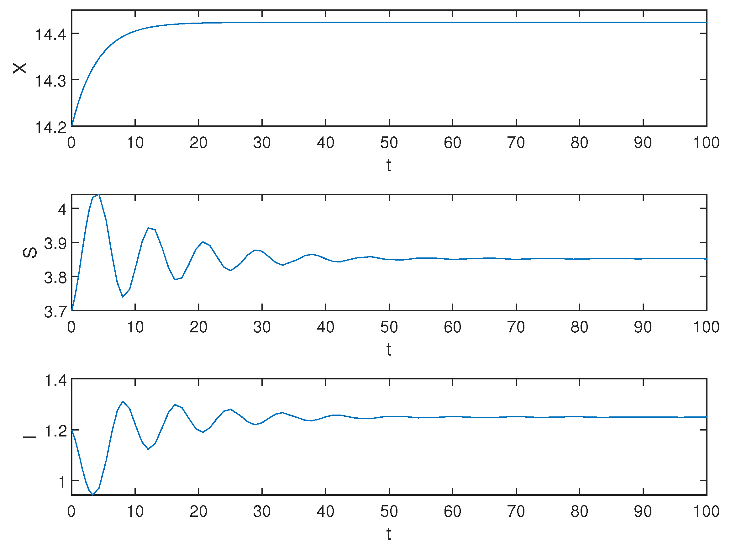
Then, we select the initial function [ X ( θ ) , S ( θ ) , I ( θ ) ] = [ 14.2 , 3.7 , 1.2 ] ( θ [ τ , 0 ] ) and τ = 1.1 < 1.2069 . Obviously, the equilibrium E * is locally asymptotically stable, the simulation results are shown in the following Figure 2.
Biological explanation 1: In Figure 2, X, S, and I undergo a brief period of change before stabilizing. During the initial stages, there is a sudden increase in the population of susceptible trees S, followed by a rapid decline, eventually stabilizing gradually. We speculate that this is due to the low number of pests in the early stages and people curing diseased trees, which leads to a rampant increase in the number of healthy trees. As time goes on, pests reproduce to their maximum capacity, infecting abundant tree resources and limiting the growth of healthy trees, resulting in a significant decrease in the number of healthy trees. Ultimately, through continued efforts in disease management and artificial reforestation activities, after undergoing some fluctuations, both S and I converge towards a certain value. Therefore, we infer that when the healing process is relatively short-term, both pests and trees will stabilize after an initial period.
When τ > 1.2069 , according to the Theorem 1, the equilibrium E * is unstable. By calculating the normal form of Hopf bifurcation, from Equations (17) and (19), we obtain K = 0.7548 + 0.2360 i , H = 0.1734 0.5544 i . According to Theorem 2, when μ < 0 , Re ( K ) μ Re ( H ) < 0 , Re ( M ) μ < 0 , the periodic solution is backward and unstable.
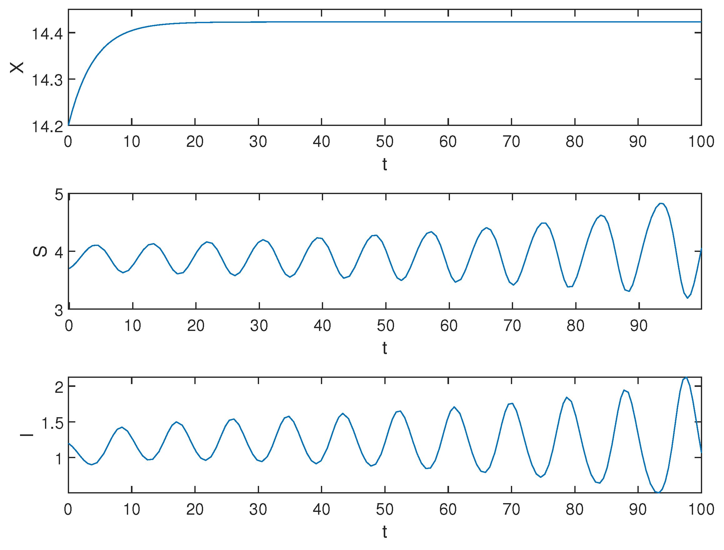
Next, we demonstrate the situation when τ = 1.22 > 1.2069 , and the simulation result is shown in Figure 3.
Biological explanation 2: From Figure 3, X is asymptotically stable, showing that the number of pests is stable at a certain number, and we can see that the amplitude of S and I fluctuations is increasing, indicating an unstable trend. We speculate that this may be due to a prolonged healing duration, resulting in many infected trees not being able to heal in time and eventually dying. The large number of dead trees increases the ability of pests to infect healthy trees. When the number of healthy trees is reduced to a certain extent, the pest’s ability to infect gradually declines due to the decrease in available hosts for the pest. Meanwhile, since the rate of artificial planting exceeds the mortality rate of trees, the number of healthy trees slowly recovers until it surpasses its original count. Due to insufficient control over the pest population, when there are enough healthy trees again, their ability to invade will recover and they initiate a new infestation, thus continuing the unstable trend.
Planted forests play a crucial role in addressing global climate change and are also valued globally for their numerous ecosystem services. The contributions of stand characteristics to carbon sequestration potential are triple that of climate variables for Larix spp. plantations in northeast China [31]. Increasing the artificial planting rate R is beneficial for carbon sequestration. The following discussion focuses on the impact of increasing this rate on the system (1).
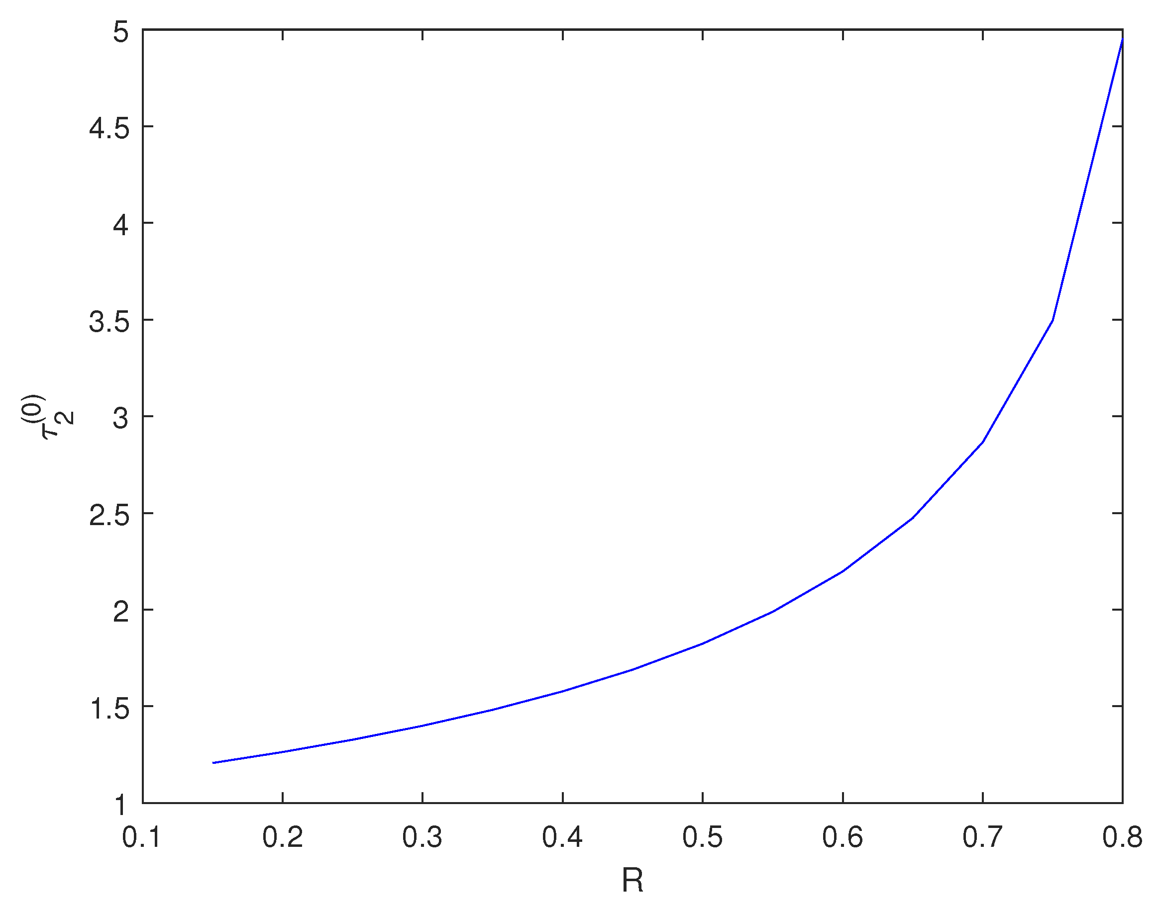
With other parameters remaining constant, through calculation, we find that when R ( 0 , 0.81 ] , the Equation (6) has two positive real roots. We choose R [ 0.15 , 0.8 ] to explore the impact of changing R on τ 2 ( 0 ) . Figure 4 shows the impact of changing R on τ 2 ( 0 ) .
Biological explanation 3: From Figure 4, we can see that as the planting rate R increases, the critical τ 2 ( 0 ) also increases. This indicates that the critical time required for healing trees becomes longer. We speculate that this phenomenon can be attributed to the “resistant stability" of the forest system. When there are a large number of trees, even if some become sick or die, other healthy trees can still perform necessary ecological functions and maintain their functional and structural capabilities. Individual sick trees will not have a significant impact on the entire ecosystem. Therefore, with an increase in artificial planting rate R, the number of trees in the forest increases and prolongs the critical time for healing.
When R > 0.81 , Equation (6) does not have positive roots. We take R = 0.85 for the simulation, to re-simulate again using the following parameters:
r = 0.78 , N = 45 , β 1 = 0.33 , β 2 = 0.12 , γ = 0.88 , k = 0.15 , M = 0.2 , R = 0.85 .
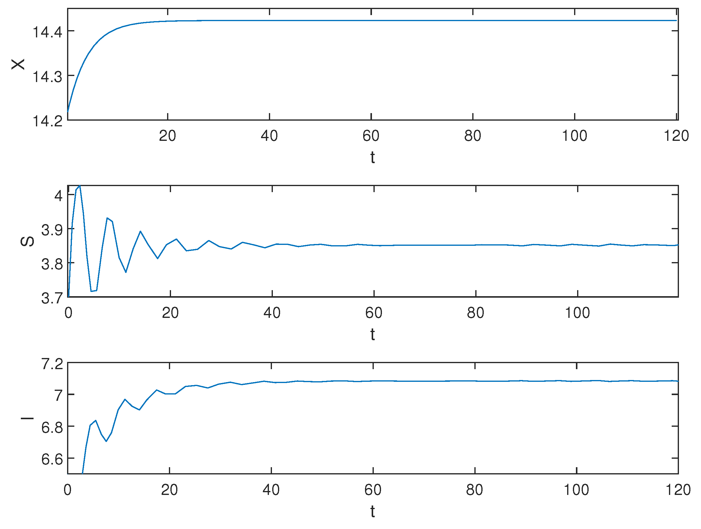
We calculate the equilibrium E * = ( 14.4231 , 3.8519 , 7.0833 ) of system (1). According to Equation (6), we find ( a 2 2 a γ 2 a β 2 ) 2 4 a 2 β 2 2 = 0.1071 < 0 and a 2 2 a γ 2 a β 2 = 0.2962 < 0 , Equation (6) does not have positive real roots, so the Hopf bifurcation does not occur near the equilibrium E * of system (1) at this time. The equilibrium E * of system (1) is always locally asymptotically stable for τ 0 . The equilibrium E * stability result is depicted in Figure 5 when τ = 2.2 .
Biological explanation 4: From Figure 5, we can see that X, S, and I eventually stabilize, even after increasing the time to cure the trees. We speculate that this is due to the strong resistance stability of the forest system under extremely high artificial planting rates R, ensuring that the system can reach a stable state.
After the above simulation results, we give some suggestions: by controlling the healing time within the critical time, the forest will eventually stabilize. However, if the healing time exceeds the critical time, this may lead to instability in the forest system. Increasing the rate of artificial planting of trees not only extends the critical time and reduces pressure on trees for recovery but also enhances carbon sequestration in forests. Therefore, people should pay more attention to and invest in artificial tree planting.

6. Conclusions

In this paper, we established a delayed differential equation model for the damage caused by Ips subelongatus Motschulsky to Larix spp. based on its biological characteristics. We investigated the stability of the equilibrium and the existence of Hopf bifurcation in the system, calculated the normal form of Hopf bifurcation by using the multiple time scale method, and analyzed the stability of the periodic solutions.
We simulated the changing trends of pests and trees using a group of parameters and confirmed our theoretical analysis. We used two different time delays τ to simulate what happens when the curing time is larger or smaller than the critical time delay τ 2 ( 0 ) , and provided corresponding biological explanations. It was found that when τ < τ 2 ( 0 ) , the equilibrium of system eventually tends to stabilize, while when τ > τ 2 ( 0 ) , the equilibrium of the system eventually becomes unstable. Due to the significant role of the artificial planting of trees in carbon sequestration, we found that increasing the artificial planting rate can prolong the critical time delay τ 2 ( 0 ) , thereby alleviating pressure on tree curing time for people. Moreover, when the artificial planting rate is very high, regardless of the duration required for curing, the system will eventually reach stability. Finally, we provided suggestions based on the simulation results, which suggest that people should increase their attention and investment in artificial tree planting.
Our model solely considered the temporal variable and only established the relationship among pests, susceptible trees, and infected trees. However, in reality, the infestation ability of pests is also influenced by spatial factors. Moreover, not all pests are capable of reproduction, and these non-reproducible pests have an impact on pest populations. Some scholars have provided mathematical foundations for enhancing the model with these aspects [32,33]. Next, we could incorporate spatial variables to construct a bivariate model or divide pest populations into reproducible and non-reproducible to establish a four-component multi-component system. These improvements would enable a more detailed investigation into the impact of pests on trees and allow accurately proposing control measures.

Author Contributions

Writing—original draft preparation, Z.L.; funding acquisition, Z.L. and Y.D.; methodology and supervision, Y.D. All authors have read and agreed to the published version of the manuscript.

Funding

This study was funded by a College Students Innovations Special Project funded by Northeast Forestry University of China (No. DC-2024126).

Data Availability Statement

No new data were created in this study. Data sharing is not applicable to this article.

Conflicts of Interest

The authors declare no conflicts of interest.

References

  1. Augusto, L.; Boča, A. Tree functional traits, forest biomass, and tree species diversity interact with site properties to drive forest soil carbon. Nat. Commun. 2022, 13, 1097. [Google Scholar] [CrossRef] [PubMed]
  2. Quirion, B.R.; Domke, G.M.; Walters, B.F.; Lovett, G.M.; Fargione, J.E.; Greenwood, L. Insect and disease disturbances correlate with reduced carbon sequestration in forests of the contiguous United States. Front. For. Glob. Chang. 2021, 4, 716582. [Google Scholar] [CrossRef]
  3. Kaczmarek, A.; Boguś, M.I. Fungi of entomopathogenic potential in Chytridiomycota and Blastocladiomycota, and in fungal allies of the Oomycota and Microsporidia. IMA Fungus 2021, 12, 29. [Google Scholar] [CrossRef] [PubMed]
  4. Vicente, C.S.L.; Soares, M.; Faria, J.M.S.; Ramos, A.P.; Lnácio, M.L. Insights into the role of fungi in pine wilt disease. J. Fungi 2021, 7, 780. [Google Scholar] [CrossRef] [PubMed]
  5. Dou, G.; Yan, D. Research progress on biocontrol of pine wilt disease by microorganisms. Forests 2022, 13, 1047. [Google Scholar] [CrossRef]
  6. Luo, Y.; Huang, H.; Roques, A. Early monitoring of forest wood-boring pests with remote sensing. Annu. Rev. Entomol. 2023, 68, 277–298. [Google Scholar] [CrossRef] [PubMed]
  7. Duarte, A.; Borralho, N.; Cabral, P.; Caetano, M. Recent advances in forest insect pests and diseases monitoring using UAV-based data: A systematic review. Forests 2022, 13, 911. [Google Scholar] [CrossRef]
  8. Bozzini, A.; Francini, S.; Chirici, G.; Battisti, A.; Faccoli, M. Spruce Bark Beetle Outbreak Prediction through Automatic Classification of Sentinel-2 Imagery. Forests 2023, 14, 1116. [Google Scholar] [CrossRef]
  9. Jentsch, P.C.; Bauch, C.T.; Anand, M. Fire mitigates bark beetle outbreaks in serotinous forests. Theor. Ecol. 2021, 14, 611–621. [Google Scholar] [CrossRef]
  10. Xu, W.; Chen, S.; Chen, L. Modeling of the prevention and control of forest pest. J. Biol. Syst. 2007, 15, 539–550. [Google Scholar] [CrossRef]
  11. Kishi, S.; Sun, J.; Kawaguchi, A.; Ochi, S.; Yoshida, M.; Yamanaka, T. Characteristic features of statistical models and machine learning methods derived from pest and disease monitoring datasets. R. Soc. Open Sci. 2023, 10, 230079. [Google Scholar] [CrossRef] [PubMed]
  12. Gutiérrez-Jara, J.P.; Vogt-Geisse, K.; Correa, M.C.G.; Vilches-Ponce, K.; Pérez, L.M.; Chowell, G. Modeling the impact of agricultural mitigation measures on the spread of Sharka disease in sweet cherry orchards. Plants 2023, 12, 3442. [Google Scholar] [CrossRef] [PubMed]
  13. Buch, K.R.; Fefferman, N.H. Mathematical Model of Basal Sprout Production in Vector-Borne Tree Disease. Forests 2023, 14, 349. [Google Scholar] [CrossRef]
  14. Song, Y.; Peng, Y.; Zhang, T. The spatially inhomogeneous Hopf bifurcation induced by memory delay in a memory-based diffusion system. J. Differ. Equ. 2021, 300, 597–624. [Google Scholar] [CrossRef]
  15. Jiang, W.; An, Q.; Shi, J. Formulation of the normal form of Turing–Hopf bifurcation in partial functional differential equations. J. Differ. Equ. 2020, 268, 705–715. [Google Scholar] [CrossRef]
  16. Sawada, Y.; Takeuchi, Y.; Dong, Y. Stability analysis of a single-species logistic model with time delay and constant inflow. Appl. Math. Lett. 2023, 138, 108514. [Google Scholar] [CrossRef]
  17. Chen, S.; Ma, W. Integrable nonlocal PT-symmetric generalized so(3,ℝ)-mKdV equations. Commun. Theor. Phys. 2023, 75, 125003. [Google Scholar] [CrossRef]
  18. Ma, W. AKNS Type Reduced Integrable Hierarchies with Hamiltonian Formulations. Rom. J. Phys. 2023, 68, 116. [Google Scholar] [CrossRef]
  19. Guo, Q.; Li, H.; Zheng, W.; Pan, J.; Lu, J.; Li, J. Analysis of genetic diversity and prediction of Larix species distribution in the Qinghai–Tibet Plateau, China. J. For. Res. 2023, 34, 705–715. [Google Scholar] [CrossRef]
  20. Mishima, K.; Hirakawa, H.; Iki, T.; Fukuda, Y.; Hirao, T.; Tamure, A.; Makoto, T. Comprehensive collection of genes and comparative analysis of full-length transcriptome sequences from Japanese larch (Larix kaempferi) and Kuril larch (Larix gmelinii var. japonica). BMC Plant Biol. 2022, 22, 470. [Google Scholar] [CrossRef]
  21. Skrzecz, I.; Perlińska, A. Current problems and tasks of forest protection in Poland. Folia For. Polonica 2018, 60, 161–172. [Google Scholar] [CrossRef]
  22. Chen, D.; Li, Y.; Zhang, Q.; Zhang, S.; Wang, H.; Zhen, Z.; Zhao, L.-L.; Kong, X.-B. Population divergence of aggregation pheromone responses in Ips subelongatus in northeastern China. Insect Sci. 2016, 23, 728–738. [Google Scholar] [CrossRef]
  23. Lee, C.Y.; Nam, Y.; Park, C.; Bae, Y.J.; Choi, W.I. Forecasting spring flight of Ips subelongatus (Coleoptera: Curculionidae: Scolytinae) in Japanese larch Larix kaempferi (Pinales: Pinaceae) forests in the Republic of Korea. Environ. Entomol. 2019, 48, 1481–1488. [Google Scholar] [CrossRef] [PubMed]
  24. Liu, X.; Wang, H.; Lu, Q.; Decock, C.; Li, Y.; Zhang, X. Taxonomy and pathogenicity of Leptographium species associated with Ips subelongatus infestations of Larix spp. in northern China, including two new species. Mycol. Prog. 2017, 16, 1–13. [Google Scholar] [CrossRef]
  25. Du, H.; Fang, J.; Shi, X.; Yu, C.; Deng, M.; Zhang, S.; Liu, F.; Zhang, Z.; Han, F.; Kong, X. Insights into the divergence of Chinese Ips bark beetles during evolutionary adaptation. Biology 2022, 11, 384. [Google Scholar] [CrossRef] [PubMed]
  26. Shi, X.; Zhang, S.; Liu, F.; Xu, F.; Zhang, F.; Guo, X.; Zhang, Z.; Kong, X.B. SEM analysis of sensilla on the mouthparts and antennae of Asian larch bark beetle Ips subelongatus. Micron 2021, 140, 102976. [Google Scholar] [CrossRef] [PubMed]
  27. Du, H.; Fang, J.; Shi, X.; Zhang, S.; Liu, F.; Yu, C.; Zhang, Z.; Kong, X. Comparative analysis of eight mitogenomes of bark beetles and their phylogenetic implications. Insects 2021, 12, 949. [Google Scholar] [CrossRef] [PubMed]
  28. Fang, J.; Liu, M.; Zhang, S.; Liu, F.; Zhang, Z.; Zhang, Q.; Kong, X. Chemical signal interactions of the bark beetle with fungal symbionts, and host/non-host trees. J. Exp. Bot. 2020, 71, 6084–6091. [Google Scholar] [CrossRef] [PubMed]
  29. Majee, S.; Adak, S.; Jana, S.; Mandal, M.; Kar, T.K. Complex dynamics of a fractional-order SIR system in the context of COVID-19. J. Appl. Math. Comput. 2022, 21, 4051–4074. [Google Scholar] [CrossRef]
  30. Li, B.; Eskandari, Z.; Avazzadeh, Z. Dynamical Behaviors of an SIR Epidemic Model with Discrete Time. Fractal Fract. 2022, 6, 659. [Google Scholar] [CrossRef]
  31. Dong, L.; Lin, X.; Bettinger, P.; Liu, Z. The contributions of stand characteristics on carbon sequestration potential are triple that of climate variables for Larix spp. plantations in northeast China. Sci. Total Environ. 2024, 911, 168726. [Google Scholar] [CrossRef] [PubMed]
  32. Shi, J.; Wang, C.; Wang, H. Diffusive Spatial Movement with Memory. J. Diff. Equ. 2020, 32, 979–1002. [Google Scholar] [CrossRef]
  33. Yu, J. Existence and stability of a unique and exact two periodic orbits for an interactive wild and sterile mosquito model. J. Diff. Equ. 2020, 269, 10395–10415. [Google Scholar] [CrossRef]
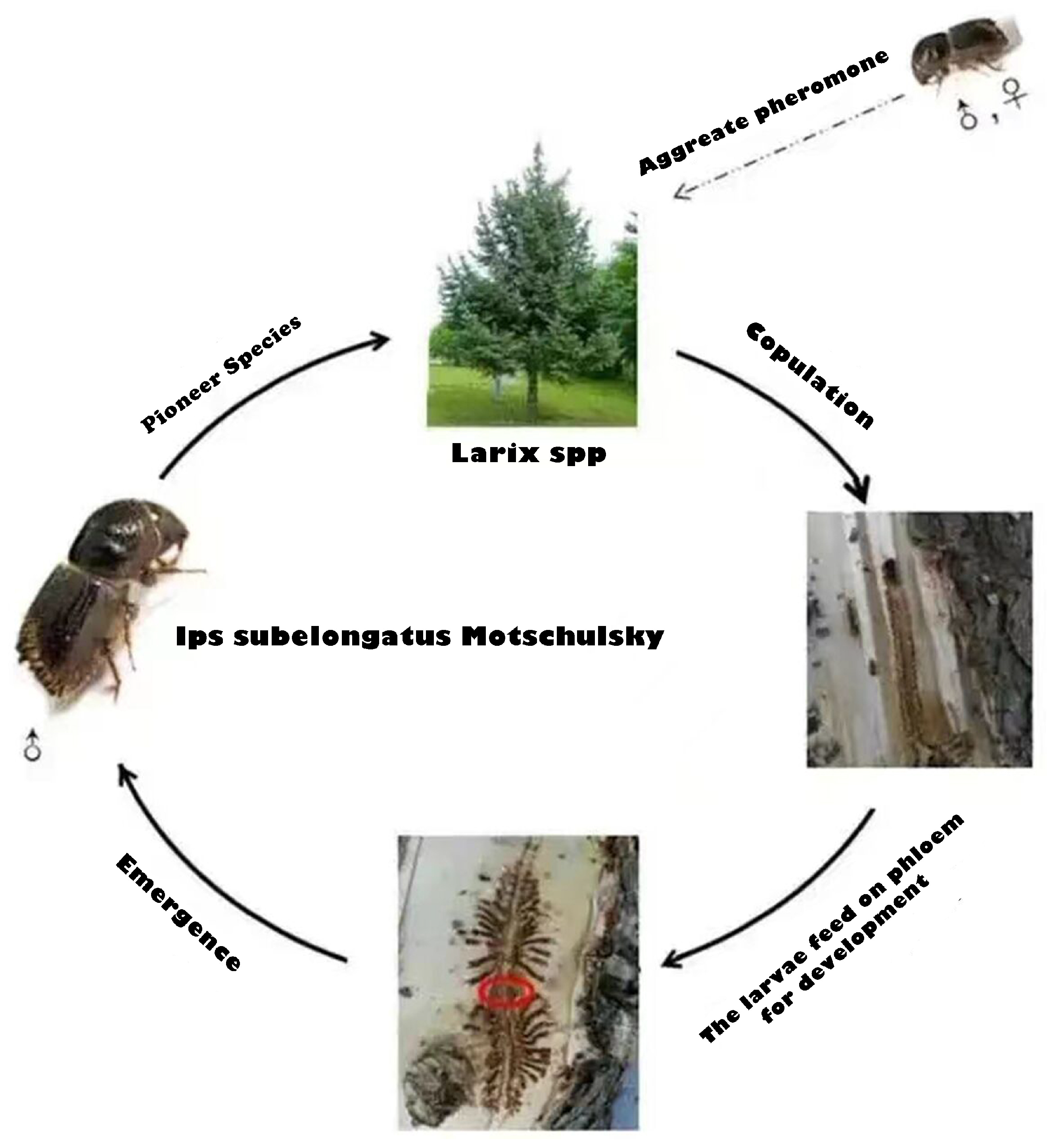
Figure 1. The infection mechanism of Ips subelongatus Motschulsky.
Axioms 13 00232 g001
Figure 2. Equilibrium E * of the system (1) is locally asymptotically stable when τ = 1.1 .
Axioms 13 00232 g002
Figure 3. Equilibrium E * of the system (1) is unstable when τ = 1.22 .
Axioms 13 00232 g003
Figure 4. τ 2 ( 0 ) varies with R.
Axioms 13 00232 g004
Figure 5. Equilibrium E * of the system (1) is locally asymptotically stable when τ = 2.2 .
Axioms 13 00232 g005
Table 1. Descriptions of the variables and parameters of the system (1).
SymbolDescriptionsUnit
XThe population size of the Ips subelongatus Motschulsky 10 7 PCS
SThe population size of susceptible Larix spp. 10 6 trees
IThe population size of infected Larix spp. 10 6 trees
rThe proliferation rate of Ips subelongatus Motschulsky-
NEnvironmental capacity of Ips subelongatus Motschulsky 10 6 PCS
β 1 The natural mortality rate of Ips subelongatus Motschulsky-
β 2 Mortality rate of infected trees-
γ The cure rate of infected trees-
τ The time required for infected trees to recover their healthMonth
kInfection rate coefficient-
MThe mortality rate caused by pests being preyed upon by natural enemies-
RThe input rate of artificially planted trees-
Disclaimer/Publisher’s Note: The statements, opinions and data contained in all publications are solely those of the individual author(s) and contributor(s) and not of MDPI and/or the editor(s). MDPI and/or the editor(s) disclaim responsibility for any injury to people or property resulting from any ideas, methods, instructions or products referred to in the content.