Exploring Stochastic Heat Equations: A Numerical Analysis with Fast Discrete Fourier Transform Techniques

Abstract

This paper presents an innovative numerical technique for specific classes of stochastic heat equations. Our approach uniquely combines a sixth-order compact finite difference algorithm with fast discrete Fourier transforms. While traditional discrete sine transforms are effective for approximating second-order derivatives, they are inadequate for first-order derivatives. To address this limitation, we introduce an innovative variant based on exponential transforms. This method is rigorously evaluated on two forms of stochastic heat equations, and the solutions are compared with those obtained using the established stochastic ten non-polynomial cubic-spline method. The results confirm the accuracy and applicability of our proposed method, highlighting its potential to enhance the numerical treatment of stochastic heat equations.

1. Introduction

The classical heat equation [1,2] shows how heat conduction is distributed in a rod, or each region over a given time. It is of fundamental importance in diverse scientific fields. In mathematics, it is used in the prototypical parabolic partial differential equation (PDE). In probability theory, the heat equation relates to the study of Brownian motion via the Fokker–Planck equation. In financial mathematics, it is used to solve the Black–Scholes PDE. The diffusion equation, a more general version of the heat equation, arises in connection with the study of chemical diffusion and other related processes.

The stochastic heat equation (SHE) is also a mathematical model that characterizes the distribution of heat in a medium over time, influenced by random fluctuations or noise. Unlike the classical heat equation, which is deterministic, the stochastic version includes a random forcing term, representing the inherent uncertainties in real-world systems, such as thermal noise. Moreover, these stochastic terms are essential for capturing the effects of randomness, which are important in various physical and mathematical systems, such as those affected by thermal fluctuations or other unpredictable forces. The stochastic heat equation combines aspects of partial differential equations with stochastic processes and provides an important tool in different fields like engineering, physics, finance, and biology [3]. The inclusion of the stochastic term makes solving the stochastic partial differential equations analytically much more complex. Therefore, numerical algorithms will be necessary to investigate their approximate solutions such as the ten non-polynomial cubic-spline (TNPCS) method [4,5], the Chebyshev wavelets with the Galerkin method [6], the Legendre polynomials together with the operational-matrix of integration [7], the finite difference approximation combined with the stochastic exponential method [8,9], spectral stochastic methods [10], quadratic spline approach [11], homotopy analysis method [12,13], Pickard method [13], finite difference (FD) and finite element methods [14,15], Tau FD approach [16], collocation method [17], collocation-Galerkin method [18], etc.

The compact finite difference (CFD) method is widely used to solve some types of the differential equations by converting them to a system of equations and solving it by the matrix inversion or any other methods [19,20]. Recently, instead of using the classical CFD schemes directly, a fast discrete Fourier transforms (FDFT) has been applied to the CFD schemes to construct new representations for the first-order, and higher-order derivatives. The FDFT method is applied, in the form of sine transforms, to the 4th-order or 6th-order CFD approach to approximate the second derivatives and used them to solve some types of the differential equations like Helmholtz equation [21], and Poisson equation [22,23,24]. On the contrary, it faces a real problem when trying to approximate the odd derivatives and as a result, it cannot be used for the differential equations that contain any odd derivatives. Following numerous attempts, we have managed to resolve this situation by using another form of the FDFT based on exponential transforms [25]. This combination between the sine and exponential transforms has been established in this study to solve the following two forms of the one-dimensional SHE as defined in [5,6] as:

$${\mathcal{U}}_t\left(x, t\right)=\rho {\mathcal{U}}_{xx}\left(x, t\right)+\sigma {\mathcal{U}}_x\left(x, t\right)+\alpha \mathcal{U}\left(x, t\right)+\beta \mathcal{U}\left(x, t\right) \dot{\mathbb{W}}\left(t\right),(\mathrm{Type} \mathrm{I})$$

(1)

or,

$${\mathcal{U}}_t\left(x, t\right)=\left(\alpha +\beta \dot{\mathbb{W}}\left(t\right)\right){\mathcal{U}}_{xx}\left(x, t\right)+\sigma {\mathcal{U}}_x\left(x, t\right),(\mathrm{Type} \mathrm{II})$$

(2)

$$\mathcal{U}\left(x, 0\right)=g\left(x\right), x\in \left[a, b\right],$$

$$\mathcal{U}\left(a, t\right)=0, \mathcal{U}\left(b, t\right)=0, t\in \left[0, T\right].$$

where $\mathcal{U}\left(x, t\right)$ is the unknown function, $\rho$, $\sigma$, $\alpha$ and $\beta$ are arbitrary constants. Also, $\dot{\mathbb{W}}\left(t\right)=\xi {\displaystyle \frac{d}{dt}}\mathbb{W}\left(t\right)$ is the Gaussian white-noise which represents a generalized derivative of the Wiener process $\mathbb{W}\left(t\right)$ with zero expectation and variance ${\xi }^2.$

Definition 1 (Wiener process) 

[26].  In mathematics, Brownian motion is also often called the Wiener process, and it is a continuous-time stochastic process characterized by the following:

• Zero initial value:  ${\mathbb{W}}_0=0$;
• Independent increments: the change   $\left({\mathbb{W}}_{t+∆t}-{\mathbb{W}}_t\right)$  is independent of the past;
• Normal distribution of increments:  $\left({\mathbb{W}}_{t+∆t}-{\mathbb{W}}_t\right)~N\left(0,∆t\right)$;
• With probability one,   $t\to \mathbb{W}\left(t\right)$  is continuous but not differentiable.

Our paper is organized as follows: The compact finite difference approach and the fast discrete Fourier transforms are introduced in Section 2 and Section 3. In Section 4, we show how to apply the proposed technique for the one-dimensional SHE. Section 5 provides the approximate solutions of the presented two cases. Finally, the conclusion is illustrated in Section 6.

2. Compact Finite Difference Scheme

Within this section, the 6th-order compact finite difference (CFD) algorithm is investigated for the first and the second order derivatives, respectively. To begin firstly, consider we have a uniform grid with $M$ subintervals, $x_i=x_0+ih$ where $h=∆x=x_{i+1}-x_i$ is the space step and $i=0, 1, 2,\dots , M$.

Secondly, the general formula of CFD approach for the 1st derivative, by using five internal nodes, can be defined as [21,22,23,24,25]:

$$\alpha {\mathcal{U}}_{i-1}^{\prime }+{\mathcal{U}}_i^{\prime }+\alpha {\mathcal{U}}_{i+1}^{\prime }=a\left({\displaystyle \frac{{\mathcal{U}}_{i+1}-{\mathcal{U}}_{i-1}}{2h}}\right)+b\left({\displaystyle \frac{{\mathcal{U}}_{i+2}-{\mathcal{U}}_{i-2}}{4h}}\right),$$

(3)

where $\alpha$, $a$ and $b$ are the constants to be determined. Applying Taylor’s approximations to Equation (3), we get the 4th order CFD approximation when $a={\displaystyle \frac{2}{3}}(\alpha +2)$ and $b={\displaystyle \frac{1}{3}}(4\alpha -1)$. The 6th order CFD approximation is obtained at $\alpha ={\displaystyle \frac{1}{3}}$, $a={\displaystyle \frac{14}{9}}$ and $b={\displaystyle \frac{1}{9}}$. Thus, 6th order CFD scheme for $u_i^{\prime }$ is:

$${\displaystyle \frac{1}{3}}{\mathcal{U}}_{i-1}^{\prime }+{\mathcal{U}}_i^{\prime }+{\displaystyle \frac{1}{3}}{\mathcal{U}}_{i+1}^{\prime }={\displaystyle \frac{14}{9}}\left({\displaystyle \frac{{\mathcal{U}}_{i+1}-{\mathcal{U}}_{i-1}}{2h}}\right)+{\displaystyle \frac{1}{9}}\left({\displaystyle \frac{{\mathcal{U}}_{i+2}-{\mathcal{U}}_{i-2}}{4h}}\right),$$

$${\mathcal{U}}_{i-1}^{\prime }+3{\mathcal{U}}_i^{\prime }+{\mathcal{U}}_{i+1}^{\prime }={\displaystyle \frac{1}{12h}}\left(-{\mathcal{U}}_{i-2}-28{\mathcal{U}}_{i-1}+28{\mathcal{U}}_{i+1}+{\mathcal{U}}_{i+2}\right).$$

(4)

Thirdly, the general formula of CFD approach for the 2nd derivative is defined as [21,22,23,24,25]:

$$\alpha {\mathcal{U}}_{i-1}^{\prime \prime }+{\mathcal{U}}_i^{\prime \prime }+\alpha {\mathcal{U}}_{i+1}^{″}=a\left({\displaystyle \frac{{\mathcal{U}}_{i-1}-2{\mathcal{U}}_i+{\mathcal{U}}_{i+1}}{h^2}}\right)+b\left({\displaystyle \frac{{\mathcal{U}}_{i-2}-2{\mathcal{U}}_i+{\mathcal{U}}_{i+2}}{4h^2}}\right),$$

(5)

where $\alpha$, $a$ and $b$ are the constants to be determined. Applying Taylor’s approximations to Equation (5), hence the 4th order CFD approximation can be achieved when $a={\displaystyle \frac{4}{3}}(1-\alpha )$ and $b={\displaystyle \frac{1}{3}}(10\alpha -1)$. Also, the 6th-order CFD approximation is given at $\alpha ={\displaystyle \frac{2}{11}}$, $a={\displaystyle \frac{12}{11}}$ and $b={\displaystyle \frac{3}{11}}$. Thus, 6th order CFD scheme for $u_i^{\prime \prime }$ is:

$${\displaystyle \frac{2}{11}}{\mathcal{U}}_{i-1}^{\prime \prime }+{\mathcal{U}}_i^{\prime \prime }+{\displaystyle \frac{2}{11}}{\mathcal{U}}_{i+1}^{\prime \prime }={\displaystyle \frac{12}{11}}\left({\displaystyle \frac{{\mathcal{U}}_{i-1}-2{\mathcal{U}}_i+{\mathcal{U}}_{i+1}}{h^2}}\right)+{\displaystyle \frac{3}{11}}\left({\displaystyle \frac{{\mathcal{U}}_{i-2}-2{\mathcal{U}}_i+{\mathcal{U}}_{i+2}}{4h^2}}\right),$$

$$2{\mathcal{U}}_{i-1}^{\prime \prime }+11{\mathcal{U}}_i^{\prime \prime }+2{\mathcal{U}}_{i+1}^{\prime \prime }={\displaystyle \frac{3}{4h^2}}\left({\mathcal{U}}_{i-2}+16{\mathcal{U}}_{i-1}-34{\mathcal{U}}_i+16{\mathcal{U}}_{i+1}+{\mathcal{U}}_{i+2}\right).$$

(6)

3. Structure of CFD Scheme Based on Fast Discrete Fourier Transforms

In this context, the fast discrete Fourier transforms (FDFT) are applied to the CFD schemes discussed in Section 2, to derive new representations for the first and the second order derivatives. For this purpose, we need to construct a uniform mesh with $M_x+1$ nodes, $x_i=x_0+i{h}_x$ where $h_x=∆x$ is the space step, $x_0=a$, $x_n=b$ and $i=0, 1, 2,\dots , M_x$. Also, taking into consideration the 6th order CFD Equations (4) and (5), then

$${\mathcal{U}}_{i-1}^x+3{\mathcal{U}}_i^x+{\mathcal{U}}_{i+1}^x={\displaystyle \frac{1}{12h}}\left({-{\mathcal{U}}_{i-2}-28\mathcal{U}}_{i-1}+28{\mathcal{U}}_{i+1}+{\mathcal{U}}_{i+2}\right),$$

(7)

$$2{\mathcal{U}}_{i-1}^{xx}+11{\mathcal{U}}_i^{xx}+2{\mathcal{U}}_{i+1}^{xx}={\displaystyle \frac{3}{4h_x^2}}\left({\mathcal{U}}_{i-2}+16{\mathcal{U}}_{i-1}-34{\mathcal{U}}_i+16{\mathcal{U}}_{i+1}+{\mathcal{U}}_{i+2}\right).$$

(8)

The one-dimensional (1D) discrete sine transforms (DST) for ${\mathcal{U}}_i$ and its inverse for ${\widehat{\mathcal{U}}}_p$ are given as in [21,22,24] as follows:

$${\mathcal{U}}_i={\sum }_{p=1}^{M_x-1}{\widehat{\mathcal{U}}}_p\sin \left({\displaystyle \frac{\pi \left(i\right)p}{M_x}}\right),$$

(9)

$${\widehat{\mathcal{U}}}_p={\displaystyle \frac{2}{M_x}}{\sum }_{i=1}^{M_x-1}{\mathcal{U}}_i\sin \left({\displaystyle \frac{\pi \left(i\right)p}{M_x}}\right).$$

(10)

Applying (9) to Equation (8) leads to

$$\begin{array}{c}2{\sum }_{p=1}^{M_x-1}{\widehat{\mathcal{U}}}_p^{xx}\sin \left({\displaystyle \frac{\pi \left(i-1\right)p}{M_x}}\right)+11{\sum }_{p=1}^{M_x-1}{\widehat{\mathcal{U}}}_p^{xx}\sin \left({\displaystyle \frac{\pi \left(i\right)p}{M_x}}\right)+\\ 2\sum _{p=1}^{M_x-1}{\widehat{\mathcal{U}}}_p^{xx}\sin \left({\displaystyle \frac{\pi \left(i+1\right)p}{M_x}}\right)={\displaystyle \frac{3}{4h_x^2}}[\sum _{p=1}^{M_x-1}{\widehat{\mathcal{U}}}_p\sin \left({\displaystyle \frac{\pi \left(i-2\right)p}{M_x}}\right)+\\ 16\sum _{p=1}^{M_x-1}{\widehat{\mathcal{U}}}_p\sin \left({\displaystyle \frac{\pi \left(i-1\right)p}{M_x}}\right)-34\sum _{p=1}^{M_x-1}{\widehat{\mathcal{U}}}_p\sin \left({\displaystyle \frac{\pi \left(i\right)p}{M_x}}\right)+\\ 16\sum _{p=1}^{M_x-1}{\widehat{\mathcal{U}}}_p\sin \left({\displaystyle \frac{\pi \left(i+1\right)p}{M_x}}\right)+\sum _{p=1}^{M_x-1}{\widehat{\mathcal{U}}}_p\sin \left({\displaystyle \frac{\pi \left(i+2\right)p}{M_x}}\right)],\\ \sum _{p=1}^{M_x-1}{\widehat{\mathcal{U}}}_p^{xx}\left[2\sin \left({\displaystyle \frac{\pi \left(i-1\right)p}{M_x}}\right)+11\sin \left({\displaystyle \frac{\pi \left(i\right)p}{M_x}}\right)+2\sin \left({\displaystyle \frac{\pi \left(i+1\right)p}{M_x}}\right)\right]=\\ {\displaystyle \frac{3}{4h_x^2}}\sum _{p=1}^{M_x-1}{\widehat{\mathcal{U}}}_p[\sin \left({\displaystyle \frac{\pi \left(i-2\right)p}{M_x}}\right)+16\sin \left({\displaystyle \frac{\pi \left(i-1\right)p}{M_x}}\right)-34\sin \left({\displaystyle \frac{\pi \left(i\right)p}{M_x}}\right)+\\ 16\sin \left({\displaystyle \frac{\pi \left(i+1\right)p}{M_x}}\right)+\sin \left({\displaystyle \frac{\pi \left(i+2\right)p}{M_x}}\right)],\end{array}$$

After simplifications,

$$\left[4\cos \left({\displaystyle \frac{p\pi }{M_x}}\right)+11\right]{\widehat{\mathcal{U}}}_p^{xx}={\displaystyle \frac{3}{2h_x^2}}\left[\cos \left({\displaystyle \frac{2p\pi }{M_x}}\right)+16\cos \left({\displaystyle \frac{p\pi }{M_x}}\right)-17\right]{\widehat{\mathcal{U}}}_p,$$

Hence,

$${\widehat{\mathcal{U}}}_p^{xx}={\displaystyle \frac{3}{2h_x^2}}\left[{\displaystyle \frac{\cos \left(\frac{2p\pi }{M_x}\right)+16\cos \left(\frac{p\pi }{M_x}\right)-17}{4\cos \left(\frac{p\pi }{M_x}\right)+11}}\right]{\widehat{\mathcal{U}}}_p.$$

(11)

Since the discrete sine transform failed to determine an approximation for ${\widehat{\mathcal{U}}}_p^x$ using Equation (7). Thus, we need to define another formula of discrete Fourier transform to achieve this approximation, which can be obtained by using the discrete exponential transforms (DET) defined as:

$${\mathcal{U}}_i={\sum }_{p=1}^{M_x}{\widehat{\mathcal{U}}}_p e^{\mathbb{i}\left({\displaystyle \frac{2\pi \left(i\right)p}{M_x}}\right)},$$

(12)

$${\widehat{\mathcal{U}}}_p={\displaystyle \frac{1}{M_x}}{\sum }_{i=1}^{M_x-1}{\mathcal{U}}_i e^{\mathbb{i}\left({\displaystyle \frac{2\pi \left(i\right)p}{M_x}}\right)}.$$

(13)

Applying (12) to Equation (7) leads to

$$\begin{array}{c}\sum _{p=1}^{M_x}{\widehat{\mathcal{U}}}_p^x e^{\mathbb{i}\left({\displaystyle \frac{2\pi \left(i-1\right)p}{M_x}}\right)}+3\sum _{p=1}^{M_x}{\widehat{\mathcal{U}}}_p^x e^{\mathbb{i}\left({\displaystyle \frac{2\pi \left(i\right)p}{M_x}}\right)}+\sum _{p=1}^{M_x}{\widehat{\mathcal{U}}}_p^x e^{\mathbb{i}\left({\displaystyle \frac{2\pi \left(i+1\right)p}{M_x}}\right)}=\\ {\displaystyle \frac{1}{12h_x}}(-\sum _{p=1}^{M_x}{\widehat{\mathcal{U}}}_p e^{\mathbb{i}\left({\displaystyle \frac{2\pi \left(i-2\right)p}{M_x}}\right)}-28\sum _{p=1}^{M_x}{\widehat{\mathcal{U}}}_p e^{\mathbb{i}\left({\displaystyle \frac{2\pi \left(i-1\right)p}{M_x}}\right)}+\\ 28\sum _{p=1}^{M_x}{\widehat{\mathcal{U}}}_p e^{\mathbb{i}\left({\displaystyle \frac{2\pi \left(i+1\right)p}{M_x}}\right)}+\sum _{p=1}^{M_x}{\widehat{\mathcal{U}}}_p e^{\mathbb{i}\left({\displaystyle \frac{2\pi \left(i+2\right)p}{M_x}}\right)}),\end{array}$$

$$\begin{array}{c}\sum _{p=1}^{M_x}\left[e^{\mathbb{i}\left({\displaystyle \frac{2\pi \left(i-1\right)p}{M_x}}\right)}+3e^{\mathbb{i}\left({\displaystyle \frac{2\pi \left(i\right)p}{M_x}}\right)}+e^{\mathbb{i}\left({\displaystyle \frac{2\pi \left(i+1\right)p}{M_x}}\right)}\right]{\widehat{\mathcal{U}}}_p^x=\\ {\displaystyle \frac{1}{12h_x}}\sum _{p=1}^{M_x}[-e^{\mathbb{i}\left({\displaystyle \frac{2\pi \left(i-2\right)p}{M_x}}\right)}-28e^{\mathbb{i}\left({\displaystyle \frac{2\pi \left(i-1\right)p}{M_x}}\right)}+28e^{\mathbb{i}\left({\displaystyle \frac{2\pi \left(i+1\right)p}{M_x}}\right)}+\\ e^{\mathbb{i}\left({\displaystyle \frac{2\pi \left(i+2\right)p}{M_x}}\right)}]{\widehat{\mathcal{U}}}_p,\end{array}$$

$$\begin{array}{c}\sum _{p=1}^{M_x}{e}^{\mathbb{i}\left({\displaystyle \frac{2\pi \left(i\right)p}{M_x}}\right)}\left[\left(e^{\mathbb{i}\left({\displaystyle \frac{-2\pi p}{M_x}}\right)}+e^{\mathbb{i}\left({\displaystyle \frac{2\pi p}{M_x}}\right)}\right)+3\right]{\widehat{\mathcal{U}}}_p^x=\\ {\displaystyle \frac{1}{12h_x}}\sum _{p=1}^{M_x}{e}^{\mathbb{i}\left({\displaystyle \frac{2\pi \left(i\right)p}{M_x}}\right)}\left[\left(-e^{\mathbb{i}\left({\displaystyle \frac{-4\pi p}{M_x}}\right)}+e^{\mathbb{i}\left({\displaystyle \frac{4\pi p}{M_x}}\right)}\right)+28\left(-e^{\mathbb{i}\left({\displaystyle \frac{-2\pi p}{M_x}}\right)}+e^{\mathbb{i}\left({\displaystyle \frac{2\pi p}{M_x}}\right)}\right)\right]{\widehat{\mathcal{U}}}_p\end{array}$$

Since $\left(e^{\mathbb{i}\left({\displaystyle \frac{-2\pi p}{M_x}}\right)}+e^{\mathbb{i}\left({\displaystyle \frac{2\pi p}{M_x}}\right)}\right)=2\cos \left({\displaystyle \frac{2\pi p}{M_x}}\right)$, $\left(-e^{\mathbb{i}\left({\displaystyle \frac{-2\pi p}{M_x}}\right)}+e^{\mathbb{i}\left({\displaystyle \frac{2\pi p}{M_x}}\right)}\right)=2\mathbb{i}\sin \left({\displaystyle \frac{2\pi p}{M_x}}\right)$, and $\left(-e^{\mathbb{i}\left({\displaystyle \frac{-4\pi p}{M_x}}\right)}+e^{\mathbb{i}\left({\displaystyle \frac{4\pi p}{M_x}}\right)}\right)=2\mathbb{i}\sin \left({\displaystyle \frac{4\pi p}{M_x}}\right)$, then

$$\begin{array}{c}\sum _{p=1}^{M_x}{e}^{\mathbb{i}\left({\displaystyle \frac{2\pi \left(i\right)p}{M_x}}\right)}\left[2\cos \left({\displaystyle \frac{2p\pi }{M_x}}\right)+3\right]{\widehat{\mathcal{U}}}_p^x=\\ {\displaystyle \frac{2\mathbb{i}}{12h_x}}\sum _{p=1}^{M_x}{e}^{\mathbb{i}\left({\displaystyle \frac{2\pi \left(i\right)p}{M_x}}\right)}\left[\sin \left({\displaystyle \frac{4p\pi }{M_x}}\right)+28\sin \left({\displaystyle \frac{2p\pi }{M_x}}\right)\right]{\widehat{\mathcal{U}}}_p,\end{array}$$

since the expression $\sum _{p=1}^{M_x}{e}^{\mathbb{i}\left({\displaystyle \frac{2\pi \left(i\right)p}{M_x}}\right)}$ exists in both sides of the above equation, then by expanding it and comparing the terms at each value of $p$. Hence, the next formula can be used to represent the above equation at any value of $p$:

$$\left[2\cos \left({\displaystyle \frac{2p\pi }{M_x}}\right)+3\right]{\widehat{\mathcal{U}}}_p^x={\displaystyle \frac{\mathbb{i}}{6h_x}}\left[\sin \left({\displaystyle \frac{4p\pi }{M_x}}\right)+28\sin \left({\displaystyle \frac{2p\pi }{M_x}}\right)\right]{\widehat{\mathcal{U}}}_p,$$

Hence,

$${\widehat{\mathcal{U}}}_p^x={\displaystyle \frac{\mathbb{i}}{6h_x}}\left[{\displaystyle \frac{\sin \left(\frac{4p\pi }{M_x}\right)+28\sin \left(\frac{2p\pi }{M_x}\right)}{2\cos \left(\frac{2p\pi }{M_x}\right)+3}}\right]{\widehat{\mathcal{U}}}_p.$$

(14)

4. Numerical Approximations of the Stochastic Heat Equations

In this section, we show how to use the fast discrete sine and exponential transforms to solve the two given formulas of the stochastic heat equations in one dimension. To begin, consider $t_j=j{h}_t$, where $h_t=∆t$ is the time step, and $j=0, 1, 2,\dots , T$. Also, assume that $\mathcal{U}=\mathcal{U}\left(x, t\right)$, ${\mathcal{U}}_t={\mathcal{U}}_t\left(x, t\right)$, ${\mathcal{U}}_x={\mathcal{U}}_x\left(x, t\right)$, ${\mathcal{U}}_{xx}={\mathcal{U}}_{xx}\left(x, t\right)$ and $\mathbb{n}\left(t\right)=\dot{\mathbb{W}}\left(t\right)$; then, Equations (1) and (2) can be written as:

$${\mathcal{U}}_t=\rho {\mathcal{U}}_{xx}+\sigma {\mathcal{U}}_x+\left(\alpha +\beta \mathbb{n}\left(t\right)\right)\mathcal{U},(\mathrm{Type} \mathrm{I})$$

(15)

or,

$${\mathcal{U}}_t=\left(\alpha +\beta \mathbb{n}\left(t\right)\right){\mathcal{U}}_{xx}+\sigma {\mathcal{U}}_x,(\mathrm{Type} \mathrm{II})$$

(16)

Then, by using the finite difference (FD), ${\mathcal{U}}_t$ and $\mathbb{n}\left(t\right)$ can be represented numerically for $\xi =1$ and $j=0, 1, 2, \dots ,T$ as: ${\left({\mathcal{U}}_t\right)}_i^j={\displaystyle \frac{1}{h_t}}\left({\mathcal{U}}_i^{j+1}-{\mathcal{U}}_i^j\right)$, and $\mathbb{n}\left(t\right)={\displaystyle \frac{1}{h_t}}\left({\mathbb{W}}^{j+1}-{\mathbb{W}}^j\right)$. In addition, applying the Crank–Nicolson (CN) method to Equations (15) and (16),

$$\left({\displaystyle \frac{{\mathcal{U}}_i^{j+1}-{\mathcal{U}}_i^j}{h_t}}\right)={\displaystyle \frac{\rho }{2}}\left({\left({\mathcal{U}}_{xx}\right)}_i^{j+1}+{\left({\mathcal{U}}_{xx}\right)}_i^j\right)+{\displaystyle \frac{\sigma }{2}}\left({\left({\mathcal{U}}_x\right)}_i^{j+1}+{\left({\mathcal{U}}_x\right)}_i^j\right)+$$

$${\displaystyle \frac{1}{2}}\left(\alpha +\beta \mathbb{n}\left(t\right)\right)\left({\mathcal{U}}_i^{j+1}+{\mathcal{U}}_i^j\right),$$

$${\mathcal{U}}_i^{j+1}-\left({\displaystyle \frac{\rho h_t}{2}}\right){\left({\mathcal{U}}_{xx}\right)}_i^{j+1}-\left({\displaystyle \frac{\sigma h_t}{2}}\right){\left({\mathcal{U}}_x\right)}_i^{j+1}-{\displaystyle \frac{h_t}{2}}\left(\alpha +{\displaystyle \frac{\beta }{h_t}} \left({\mathbb{W}}^{j+1}-{\mathbb{W}}^j\right)\right){\mathcal{U}}_i^{j+1}$$

$$={\mathcal{U}}_i^j+\left({\displaystyle \frac{\rho h_t}{2}}\right){\left({\mathcal{U}}_{xx}\right)}_i^j+\left({\displaystyle \frac{\sigma h_t}{2}}\right){\left({\mathcal{U}}_x\right)}_i^j+ {\displaystyle \frac{h_t}{2}}\left(\alpha +\beta \left({\mathbb{W}}^{j+1}-{\mathbb{W}}^j\right)\right){\mathcal{U}}_i^j,(\mathrm{Type} \mathrm{I})$$

(17)

or,

$$\left({\displaystyle \frac{{\mathcal{U}}_i^{j+1}-{\mathcal{U}}_i^j}{h_t}}\right)={\displaystyle \frac{1}{2}}\left(\alpha +\beta \mathbb{n}\left(t\right)\right)\left({\left({\mathcal{U}}_{xx}\right)}_i^{j+1}+{\left({\mathcal{U}}_{xx}\right)}_i^j\right)+{\displaystyle \frac{\sigma }{2}}\left({\left({\mathcal{U}}_x\right)}_i^{j+1}+{\left({\mathcal{U}}_x\right)}_i^j\right),$$

$${\mathcal{U}}_i^{j+1}-{\displaystyle \frac{h_t}{2}}\left(\alpha +{\displaystyle \frac{\beta }{h_t}} \left({\mathbb{W}}^{j+1}-{\mathbb{W}}^j\right)\right){\left({\mathcal{U}}_{xx}\right)}_i^{j+1}-\left({\displaystyle \frac{\sigma h_t}{2}}\right){\left({\mathcal{U}}_x\right)}_i^{j+1}$$

$$={\mathcal{U}}_i^j+{\displaystyle \frac{h_t}{2}}\left(\alpha +{\displaystyle \frac{\beta }{h_t}} \left({\mathbb{W}}^{j+1}-{\mathbb{W}}^j\right)\right){\left({\mathcal{U}}_{xx}\right)}_i^j+\left({\displaystyle \frac{\sigma h_t}{2}}\right){\left({\mathcal{U}}_x\right)}_i^j,(\mathrm{Type} \mathrm{II}).$$

(18)

Assume that

$$U={\mathcal{U}}_i^{j+1}, U^x={\left({\mathcal{U}}_x\right)}_i^{j+1}, U^{xx}={\left({\mathcal{U}}_{xx}\right)}_i^{j+1}, \mathcal{w}=\alpha +{\displaystyle \frac{\beta }{h_t}} \left({\mathbb{W}}^{j+1}-{\mathbb{W}}^j\right),$$

$$G={\mathcal{U}}_i^j+\left({\displaystyle \frac{\rho h_t}{2}}\right){\left({\mathcal{U}}_{xx}\right)}_i^j+\left({\displaystyle \frac{\sigma h_t}{2}}\right){\left({\mathcal{U}}_x\right)}_i^j+\left({\displaystyle \frac{h_t\mathcal{w}}{2}}\right){\mathcal{U}}_i^j,$$

and $H={\mathcal{U}}_i^j+{\displaystyle \frac{h_t}{2}}\left(\alpha +{\displaystyle \frac{\beta }{h_t}}\left({\mathbb{W}}^{j+1}-{\mathbb{W}}^j\right)\right){\left({\mathcal{U}}_{xx}\right)}_i^j+\left({\displaystyle \frac{\sigma h_t}{2}}\right){\left({\mathcal{U}}_x\right)}_i^j$.

Then, Equations (17) and (18) can be reduced to the following forms

$$\left(1-\left({\displaystyle \frac{h_t}{2}}\right)\mathcal{w}\right)U-\left({\displaystyle \frac{\rho h_t}{2}}\right)U^{xx}-\left({\displaystyle \frac{\sigma h_t}{2}}\right)U^x=G,(\mathrm{Type} \mathrm{I})$$

(19)

or,

$$U-\left({\displaystyle \frac{h_t}{2}}\right)\mathcal{w}{U}^{xx}-\left({\displaystyle \frac{\sigma h_t}{2}}\right)U^x=H,(\mathrm{Type} \mathrm{II}).$$

(20)

In addition, by discretizing Equations (19) and (20), we obtain

$$\left(1-\left({\displaystyle \frac{h_t}{2}}\right)\mathcal{w}\right)U_i-\left({\displaystyle \frac{\rho h_t}{2}}\right)U_i^{xx}-\left({\displaystyle \frac{\sigma h_t}{2}}\right)U_i^x=G_i,(\mathrm{Type} \mathrm{I})$$

(21)

or,

$$U_i-\left({\displaystyle \frac{h_t}{2}}\right)\mathcal{w}{U}_i^{xx}-\left({\displaystyle \frac{\sigma h_t}{2}}\right)U_i^x=H_i,(\mathrm{Type} \mathrm{II}).$$

(22)

Utilizing the inverse-Fourier transform for Equations (21) and (22),

$$\left(1-\left({\displaystyle \frac{h_t}{2}}\right)\mathcal{w}\right){\widehat{U}}_p-\left({\displaystyle \frac{\rho h_t}{2}}\right){\widehat{U}}_p^{xx}-\left({\displaystyle \frac{\sigma h_t}{2}}\right){\widehat{U}}_p^x={\widehat{G}}_p,(\mathrm{Type} \mathrm{I})$$

(23)

or,

$${\widehat{U}}_p-\left({\displaystyle \frac{h_t}{2}}\right)\mathcal{w}{\widehat{U}}_p^{xx}-\left({\displaystyle \frac{\sigma h_t}{2}}\right){\widehat{U}}_p^x={\widehat{H}}_p,(\mathrm{Type} \mathrm{II}).$$

(24)

Now, applying the approximations of ${\widehat{U}}_p^x$ and ${\widehat{U}}_p^{xx}$ from Equations (19) and (22) into Equations (23) and (24), we have

$${\widehat{U}}_p={\displaystyle \frac{2 {\widehat{G}}_p}{\left(2-h_t \mathcal{w}\right)-\left(\frac{3\rho h_t}{2h_x^2}\right)\left[\frac{\cos \left(\frac{2p\pi }{M_x}\right)+16\cos \left(\frac{p\pi }{M_x}\right)-17}{4\cos \left(\frac{p\pi }{M_x}\right)+11}\right]-\left(\frac{\mathbb{i} \sigma h_t}{6h_x}\right)\left[\frac{\sin \left(\frac{4p\pi }{M_x}\right)+28\sin \left(\frac{2p\pi }{M_x}\right)}{2\cos \left(\frac{2p\pi }{M_x}\right)+3}\right]}},(\mathrm{Type} \mathrm{I})$$

(25)

or,

$${\widehat{U}}_p={\displaystyle \frac{2 {\widehat{H}}_p}{2-\left(\frac{3 h_t\mathcal{w}}{2h_x^2}\right)\left[\frac{\cos \left(\frac{2p\pi }{M_x}\right)+16\cos \left(\frac{p\pi }{M_x}\right)-17}{4\cos \left(\frac{p\pi }{M_x}\right)+11}\right]-\left(\frac{\mathbb{i}\sigma h_t}{6h_x}\right)\left[\frac{\sin \left(\frac{4p\pi }{M_x}\right)+28\sin \left(\frac{2p\pi }{M_x}\right)}{2\cos \left(\frac{2p\pi }{M_x}\right)+3}\right]}},(\mathrm{Type} \mathrm{II}).$$

(26)

Equations (19) and (20) can be solved by the following fast algorithm for $j=0, 1, 2,\dots , T$, and $u_0^j=u_{M_x}^j=0$:

• Firstly, obtain ${\left({\mathcal{U}}_{xx}\right)}_i^j$:

  $${\widehat{\mathcal{U}}}_p={\displaystyle \frac{2}{M_x}}{\sum }_{i=1}^{M_x-1}{\mathcal{U}}_i^j\sin \left({\displaystyle \frac{\pi \left(i\right)p}{M_x}}\right)$$

  $${\widehat{\mathcal{U}}}_p^{xx}={\displaystyle \frac{3}{2h_x^2}}\left[{\displaystyle \frac{\cos \left(\frac{2p\pi }{M_x}\right)+16\cos \left(\frac{p\pi }{M_x}\right)-17}{4\cos \left(\frac{p\pi }{M_x}\right)+11}}\right]{\widehat{\mathcal{U}}}_p$$

  $${\left({\mathcal{U}}_{xx}\right)}_i^j={\sum }_{i=1}^{M_x-1}{\widehat{\mathcal{U}}}_p^{xx}\sin \left({\displaystyle \frac{\pi \left(i\right)p}{M_x}}\right)$$

  (27)
• Secondly, obtain ${\left({\mathcal{U}}_x\right)}_i^j$:

  $${\widehat{\mathcal{U}}}_p={\displaystyle \frac{1}{M_x}}{\sum }_{i=1}^{M_x-1}{\mathcal{U}}_i^j{e}^{\mathbb{i}\left({\displaystyle \frac{2\pi \left(i\right)p}{M_x}}\right)},$$

  $${\widehat{\mathcal{U}}}_p^x={\displaystyle \frac{\mathbb{i}}{6h_x}}\left[{\displaystyle \frac{\sin \left(\frac{4p\pi }{M_x}\right)+28\sin \left(\frac{2p\pi }{M_x}\right)}{2\cos \left(\frac{2p\pi }{M_x}\right)+3}}\right]{\widehat{u}}_p,$$

  $${\left({\mathcal{U}}_x\right)}_i^j={\sum }_{i=1}^{M_x-1}{\widehat{\mathcal{U}}}_p^x\sin \left({\displaystyle \frac{\pi \left(i\right)p}{M_x}}\right),$$

  (28)
• Thirdly, obtain ${\widehat{U}}_p$ for the given SHEs:
  By applying Equations (27) and (28) to Equation (21),

  $$G_i=\left(1+\left({\displaystyle \frac{h_t}{2}}\right){\mathcal{w}}_j\right){\mathcal{U}}_i^j+\left({\displaystyle \frac{\rho h_t}{2}}\right){\left({\mathcal{U}}_{xx}\right)}_i^j+\left({\displaystyle \frac{\sigma h_t}{2}}\right){\left({\mathcal{U}}_x\right)}_i^j,$$

  $${\widehat{G}}_p={\displaystyle \frac{2}{M_x}}{\sum }_{i=1}^{M_x-1}{G}_i\sin \left({\displaystyle \frac{\pi \left(i\right)p}{M_x}}\right),$$

  $${\widehat{U}}_p={\displaystyle \frac{2 {\widehat{G}}_p}{\left(2-h_t \mathcal{w}\right)-\left(\frac{3\rho h_t}{2h_x^2}\right)\left[\frac{\cos \left(\frac{2p\pi }{M_x}\right)+16\cos \left(\frac{p\pi }{M_x}\right)-17}{4\cos \left(\frac{p\pi }{M_x}\right)+11}\right]-\left(\frac{\mathbb{i} \sigma h_t}{6h_x}\right)\left[\frac{\sin \left(\frac{4p\pi }{M_x}\right)+28\sin \left(\frac{2p\pi }{M_x}\right)}{2\cos \left(\frac{2p\pi }{M_x}\right)+3}\right]}},(\mathrm{Type} \mathrm{I}),$$

  (29)

  also, applying Equations (27) and (28) to Equation (22),

  $$H_i={\mathcal{U}}_i^j+\left({\displaystyle \frac{h_t}{2}}\right){\mathcal{w}}_j {\left({\mathcal{U}}_{xx}\right)}_i^j+\left({\displaystyle \frac{\sigma h_t}{2}}\right){\left({\mathcal{U}}_x\right)}_i^j,$$

  $${\widehat{H}}_p={\displaystyle \frac{2}{M_x}}{\sum }_{i=1}^{M_x-1}{H}_i\sin \left({\displaystyle \frac{\pi \left(i\right)p}{M_x}}\right),$$

  $${\widehat{U}}_p={\displaystyle \frac{2 {\widehat{H}}_p}{2-\left(\frac{3 h_t\mathcal{w}}{2h_x^2}\right)\left[\frac{\cos \left(\frac{2p\pi }{M_x}\right)+16\cos \left(\frac{p\pi }{M_x}\right)-17}{4\cos \left(\frac{p\pi }{M_x}\right)+11}\right]-\left(\frac{\mathbb{i}\sigma h_t}{6h_x}\right)\left[\frac{\sin \left(\frac{4p\pi }{M_x}\right)+28\sin \left(\frac{2p\pi }{M_x}\right)}{2\cos \left(\frac{2p\pi }{M_x}\right)+3}\right]}},(\mathrm{Type} \mathrm{II})$$

  (30)
• Finally, the solution for the two types of SHE at each level $j$ can be obtained by substituting ${\widehat{U}}_p$ from Equation (29) or (30) into the next equation:

  $${\mathcal{U}}_i^j=U_i={\sum }_{p=1}^{M_x-1}{\widehat{U}}_p\sin \left({\displaystyle \frac{\pi \left(i\right)p}{M_x}}\right), \mathrm{for} 1\le i\le M_x-1, \mathrm{and} 0\le j\le T.$$

  (31)

To obtain the solution of the given SHEs (1) and (2), it is essential to apply a variety of Wiener process samples. As a result, the above iterative fast algorithm should be executed $\mathcal{K}$ times, as detailed below:

• Firstly, obtain ${\left({\mathcal{U}}_{xx}\right)}_{i,\mathcal{K}}^j$:

  $${\widehat{\mathcal{U}}}_{p,\mathcal{K}}={\displaystyle \frac{2}{M_x}}{\sum }_{i=1}^{M_x-1}{\mathcal{U}}_{i,\mathcal{K}}^j\sin \left({\displaystyle \frac{\pi \left(i\right)p}{M_x}}\right),$$

  $${\widehat{\mathcal{U}}}_{p,\mathcal{K}}^{xx}={\displaystyle \frac{3}{2h_x^2}}\left[{\displaystyle \frac{\cos \left(\frac{2p\pi }{M_x}\right)+16\cos \left(\frac{p\pi }{M_x}\right)-17}{4\cos \left(\frac{p\pi }{M_x}\right)+11}}\right]{\widehat{\mathcal{U}}}_{p,\mathcal{K}},$$

  $${\left({\mathcal{U}}_{xx}\right)}_{i,\mathcal{K}}^j={\sum }_{i=1}^{M_x-1}{\widehat{\mathcal{U}}}_{p,\mathcal{K}}^{xx}\sin \left({\displaystyle \frac{\pi \left(i\right)p}{M_x}}\right),$$

  (32)
• Secondly, obtain ${\left({\mathcal{U}}_x\right)}_{i,\mathcal{K}}^j$:

  $${\widehat{\mathcal{U}}}_{p,\mathcal{K}}={\displaystyle \frac{1}{M_x}}{\sum }_{i=1}^{M_x-1}{\mathcal{U}}_{i,\mathcal{K}}^j{e}^{\mathbb{i}\left({\displaystyle \frac{2\pi \left(i\right)p}{M_x}}\right)},$$

  $${\widehat{\mathcal{U}}}_{p,\mathcal{K}}^x={\displaystyle \frac{\mathbb{i}}{6h_x}}\left[{\displaystyle \frac{\sin \left(\frac{4p\pi }{M_x}\right)+28\sin \left(\frac{2p\pi }{M_x}\right)}{2\cos \left(\frac{2p\pi }{M_x}\right)+3}}\right]{\widehat{\mathcal{U}}}_{p,\mathcal{K}},$$

  $${\left({\mathcal{U}}_x\right)}_{i,\mathcal{K}}^j={\sum }_{i=1}^{M_x-1}{\widehat{\mathcal{U}}}_{p,\mathcal{K}}^x\sin \left({\displaystyle \frac{\pi \left(i\right)p}{M_x}}\right),$$

  (33)

  $${\mathcal{w}}_{j,\mathcal{K}}=\alpha +{\displaystyle \frac{\beta }{h_t}}\left({\mathbb{W}}_{\mathcal{K}}^{j+1}-{\mathbb{W}}_{\mathcal{K}}^j\right),$$

  (34)
• Thirdly, obtain ${\widehat{U}}_{p,\mathcal{K}}$ for type I SHE:

  $$G_{i,\mathcal{K}}=\left(1+\left({\displaystyle \frac{h_t}{2}}\right){\mathcal{w}}_{j,\mathcal{K}}\right){\mathcal{U}}_{i,\mathcal{K}}^j+\left({\displaystyle \frac{\rho h_t}{2}}\right){\left({\mathcal{U}}_{xx}\right)}_{i,\mathcal{K}}^j+\left({\displaystyle \frac{\sigma h_t}{2}}\right){\left({\mathcal{U}}_x\right)}_{i,\mathcal{K}}^j,$$

  $${\widehat{G}}_{p,\mathcal{K}}={\displaystyle \frac{2}{M_x}}{\sum }_{i=1}^{M_x-1}{G}_{i,\mathcal{K}}\sin \left({\displaystyle \frac{\pi \left(i\right)p}{M_x}}\right),$$

  $${\widehat{U}}_{p,\mathcal{K}}={\displaystyle \frac{2 {\widehat{G}}_{p,\mathcal{K}}}{\left(2-h_t {\mathcal{w}}_{\mathcal{K}}\right)-\left(\frac{3\rho h_t}{2h_x^2}\right)\left[\frac{\cos \left(\frac{2p\pi }{M_x}\right)+16\cos \left(\frac{p\pi }{M_x}\right)-17}{4\cos \left(\frac{p\pi }{M_x}\right)+11}\right]-\left(\frac{\mathbb{i}\sigma h_t}{6h_x}\right)\left[\frac{\sin \left(\frac{4p\pi }{M_x}\right)+28\sin \left(\frac{2p\pi }{M_x}\right)}{2\cos \left(\frac{2p\pi }{M_x}\right)+3}\right]}}$$

  (35)
  Similarly, for type II SHE:

  $$H_{i,\mathcal{K}}={\mathcal{U}}_{i,\mathcal{K}}^j+\left({\displaystyle \frac{h_t}{2}}\right){\mathcal{w}}_{j,\mathcal{K}} {\left({\mathcal{U}}_{xx}\right)}_{i,\mathcal{K}}^j+\left({\displaystyle \frac{\sigma h_t}{2}}\right){\left({\mathcal{U}}_x\right)}_{i,\mathcal{K}}^j,$$

  $${\widehat{H}}_{p,\mathcal{K}}={\displaystyle \frac{2}{M_x}}{\sum }_{i=1}^{M_x-1}{H}_{i,\mathcal{K}}\sin \left({\displaystyle \frac{\pi \left(i\right)p}{M_x}}\right),$$

  $${\widehat{U}}_{p,\mathcal{K}}={\displaystyle \frac{2 {\widehat{H}}_{p,\mathcal{K}}}{2-\left(\frac{3 h_t {\mathcal{w}}_{\mathcal{K}}}{2h_x^2}\right)\left[\frac{\cos \left(\frac{2p\pi }{M_x}\right)+16\cos \left(\frac{p\pi }{M_x}\right)-17}{4\cos \left(\frac{p\pi }{M_x}\right)+11}\right]-\left(\frac{\mathbb{i}\sigma h_t}{6h_x}\right)\left[\frac{\sin \left(\frac{4p\pi }{M_x}\right)+28\sin \left(\frac{2p\pi }{M_x}\right)}{2\cos \left(\frac{2p\pi }{M_x}\right)+3}\right]}},$$

  (36)
• Finally, the solution of the SHES (1.1) or (1.2) is:

  $${\mathcal{U}}_{i,\mathcal{K}}^j=U_{i,\mathcal{K}}={\sum }_{p=1}^{M_x-1}{\widehat{U}}_{p,\mathcal{K}}\sin \left({\displaystyle \frac{\pi \left(i\right)p}{M_x}}\right), \mathrm{for} 1\le i\le M_x-1, \mathrm{and} 0\le j\le T.$$

  (37)

The above iterative scheme of Equations (32)– (36) can be solved for $\mathcal{K}=1$ and $j=\mathrm{0,1},2,\dots ,T$, and the same procedure can be performed for $\mathcal{K}=2,3,4,\dots$. Hence, we can obtain the expectation and the variance of the solution-sequences $\left\{{\mathcal{U}}_{i,1}^j, {\mathcal{U}}_{i,2}^j, {\mathcal{U}}_{i,3}^j,\dots ,{\mathcal{U}}_{i,\mathcal{K}}^j\right\}$ for the given stochastic heat Equations (1) and (2).

5. Numerical Results

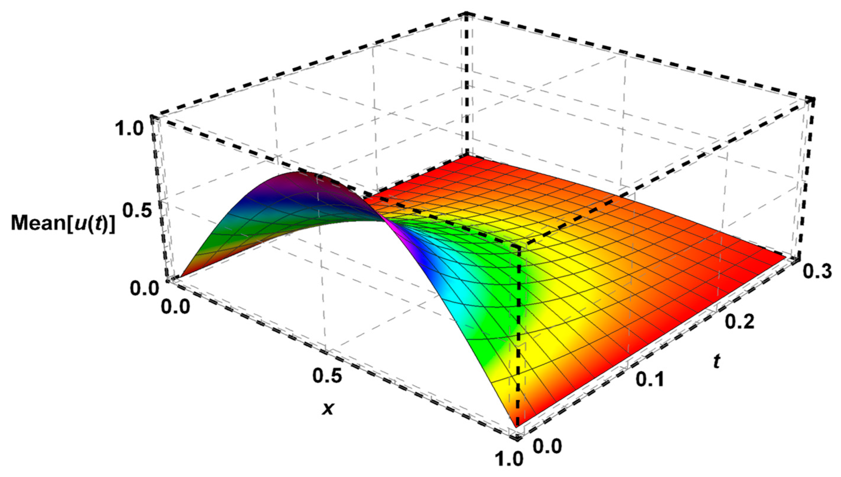
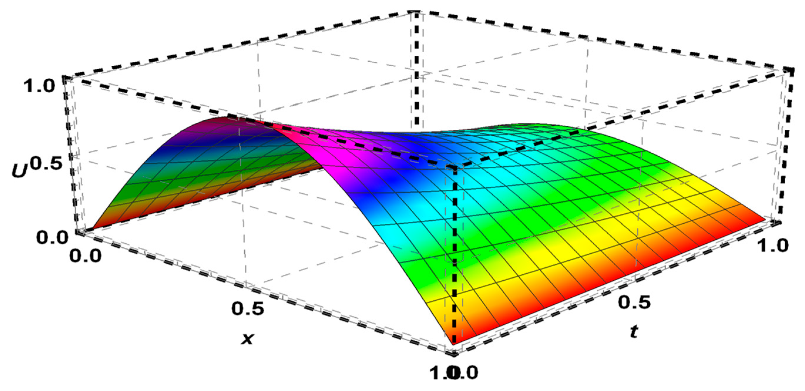
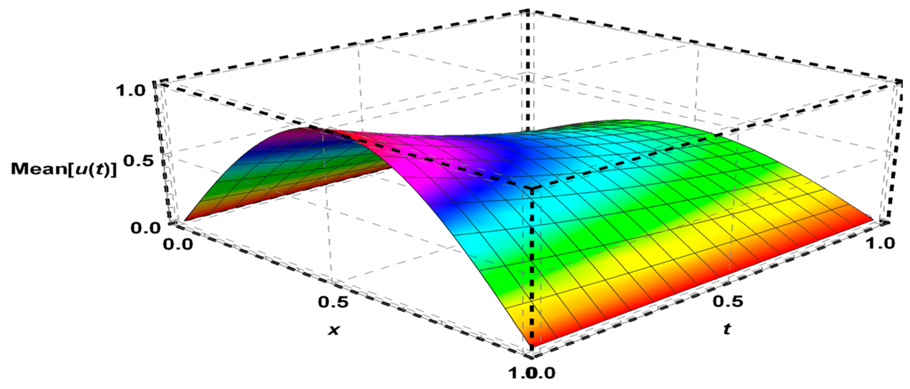
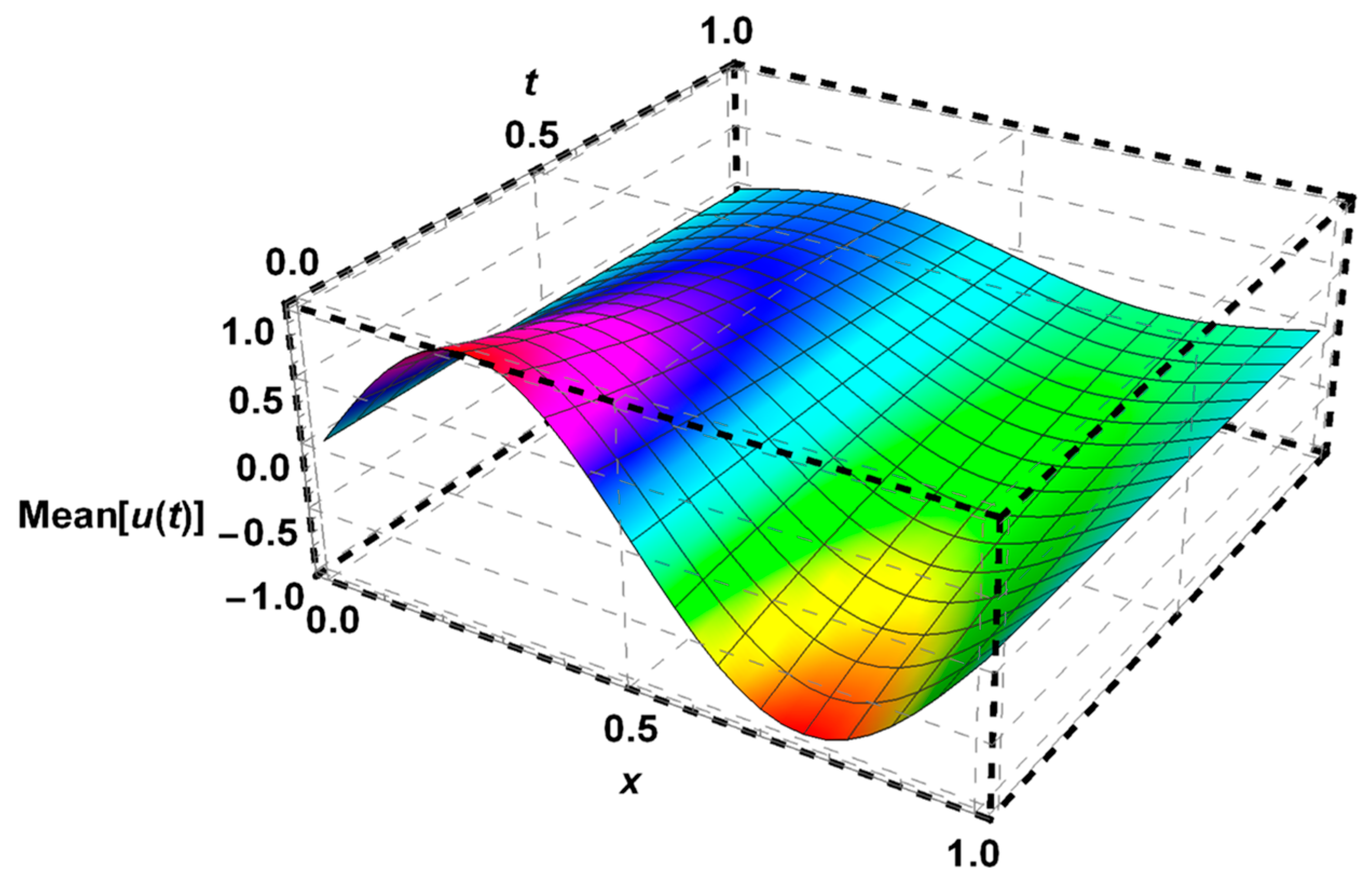
Figure 1, Figure 2, Figure 3, Figure 4, Figure 5 and Figure 6 illustrate the expectation and the variance for three stochastic heat equations of the form specified in Equation (1), using parameters set to $M_x=80$, $h_t=0.01$, and utilizing about 2000 samples of $\mathbb{W}\left(t\right)$. These figures clearly show the behaviour of the solutions, capturing both expected values and the associated variances under the influence of noise.

Figure 7, Figure 8, Figure 9, Figure 10 and Figure 11 extend this analysis to two stochastic heat equations characterized by Equation (2), with parameters set to $M_x=32$ and $h_t=0.01$, and utilizing about 2000 samples of $\mathbb{W}\left(t\right)$. The visual representation of these results emphasizes the robustness of our method in handling stochastic variability.

Table 1. The numerical results of Problem 1 for $h_t=0.01$ and $t=0.3$.

x	Method in [31]	STNPCS [5]	FDFT
No. of Noise Samples	10,000	2000	2000
$0.125$	0.020364	0.0197639	$0.0197644$
$0.250$	0.037627	0.0365191	$0.0365198$
$0.375$	0.049162	0.0477145	$0.0477154$
$0.500$	0.053213	0.0516458	$0.0516468$
$0.625$	0.049162	0.0477145	$0.0477154$
$0.750$	0.037627	0.0365191	$0.0365198$
$0.875$	0.020364	0.0197639	$0.0197644$
$1.000$	0.0	0.0	0.0

,

Table 2. The numerical results of Problem 2 for $h_t=0.01$ and $t=0.3$.

x	STNPCS [5]	FDFT
$0.125$	0.0377703	0.0358112
$0.250$	$0.069772$	0.0683866
$0.375$	$0.091155$	0.0912509
$0.500$	$0.098660$	0.0994191
$0.625$	$0.091145$	0.0912509
$0.750$	$0.069755$	0.0683866
$0.875$	$0.037751$	0.0358112
$1.000$	0.0	0.0

,

Table 3. The numerical results of Problem 3 for $h_t=0.01$ and $t=0.3$.

x	STNPCS [5]	FDFT
$0.125$	$0.013944$	$0.0139333$
$0.250$	$0.034553$	$0.0345279$
$0.375$	$0.052662$	$0.0526253$
$0.500$	$0.059676$	$0.0596333$
$0.625$	$0.052662$	$0.0526253$
$0.750$	$0.034553$	$0.0345279$
$0.875$	$0.013944$	$0.0139333$
$1.000$	0.0	0.0

and

Table 4. The numerical results of Problem 4 for $\beta =0.01$ and $t=1$.

x	STNPCS [5]	FDFT
$0.125$	$0.141702$	$0.141661$
$0.250$	$0.261831$	$0.261756$
$0.375$	$0.342099$	$0.342001$
$0.500$	$0.370285$	$0.370179$
$0.625$	$0.342099$	$0.342001$
$0.750$	$0.261831$	$0.261756$
$0.875$	$0.141702$	$0.141661$
$1.000$	0.0	0.0

provide a detailed comparison of the numerical results generated using the STNPCS [4,5,27] technique and the Fourier transform [28,29,30]. These tables quantitatively demonstrate that our proposed method significantly reduces computational time and effort. Specifically, the FDFT method consistently outperformed the STNPCS technique in terms of processing speed while maintaining a high level of accuracy.

One of the key advantages of the suggested method is its stability in the presence of increased noise. As the number of samples from the noise term rises, our approach remains reliable and produces consistent results across all five problems analysed. This stability is crucial for practical applications, where uncertainty is inherent.

Overall, the present data indicate that the FDFT algorithm is not only faster and more efficient but also enhances the reliability of numerical solutions for stochastic heat equations. This underscores the method’s potential for broader application in complex systems requiring real-time or high-frequency computations. All calculations were performed using Mathematica 12.1, ensuring a robust computational environment for our analysis.

Problem 1. 

Consider the 1D SHE [5,31] is:

$${\mathcal{U}}_t\left(x, t\right)={\mathcal{U}}_{xx}\left(x, t\right)-0.01 \mathcal{U}\left(x, t\right) \dot{\mathbb{W}}\left(t\right),$$

(38)

$$\mathcal{U}\left(x, 0\right)=\mathit{sin} \left(\pi x\right),\mathcal{U}\left(0, t\right)=\mathcal{U}\left(1, t\right)=0,x\in \left[0, 1\right],t\in \left[0, 0.3\right].$$

Figure 1 showed the mean of solutions for Problem 1, while Figure 2 illustrated a very small variance of solutions given by FDFT and STNPCS methods which indicated that the solutions using FDFT are more accurate. Also, a comparison of solutions between different methods is given in Table 1.

Problem 2. 

Consider the 1D SHE [5,31] is:

$${\mathcal{U}}_t\left(x, t\right)={\mathcal{U}}_{xx}\left(x, t\right)+2{\mathcal{U}}_x\left(x, t\right)-\left(1+0.02 \dot{\mathbb{W}}\left(t\right)\right)\mathcal{U}\left(x, t\right)$$

(39)

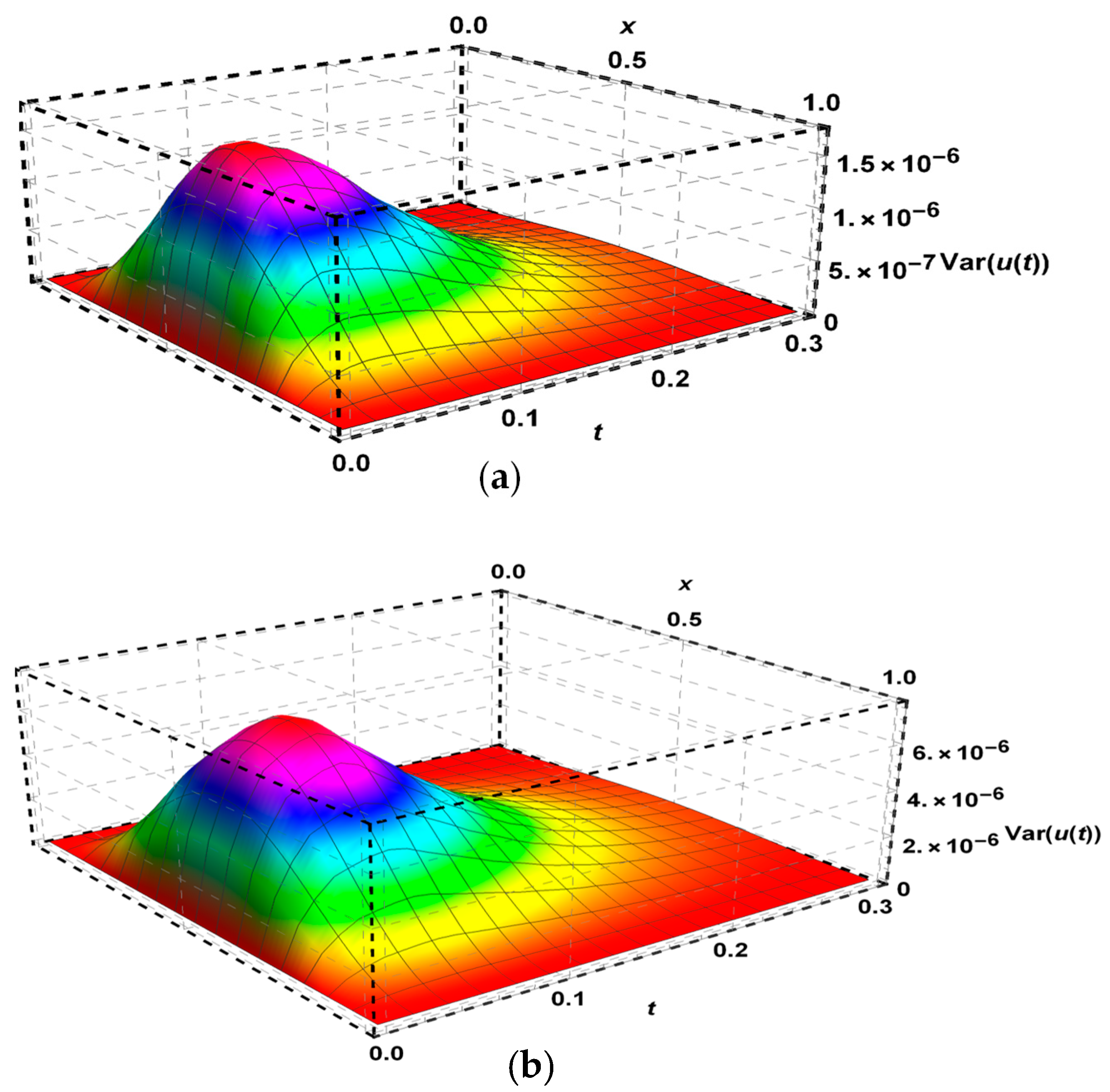
$$\mathcal{U}\left(x, 0\right)=10x\left(1-x\right), \mathcal{U}\left(0, t\right)=\mathcal{U}\left(1, t\right)=0, x\in \left[0, 1\right], t\in \left[0, 0.3\right]$$

The mean of solutions for Problem 2 is obtained by the present technique and visualized in Figure 3. The FDFT and STNPCS methods introduced its solutions in Table 2, and an $O\left(h^5\right)$ variance of solutions in Figure 4.

Problem 3. 

Consider the 1D SHE [5,31] is:

$${\mathcal{U}}_t\left(x, t\right)=0.01{\mathcal{U}}_{xx}\left(x, t\right)+0.01{\mathcal{U}}_x\left(x, t\right)-0.02 \mathcal{U}\left(x, t\right) \dot{\mathbb{W}}\left(t\right)$$

(40)

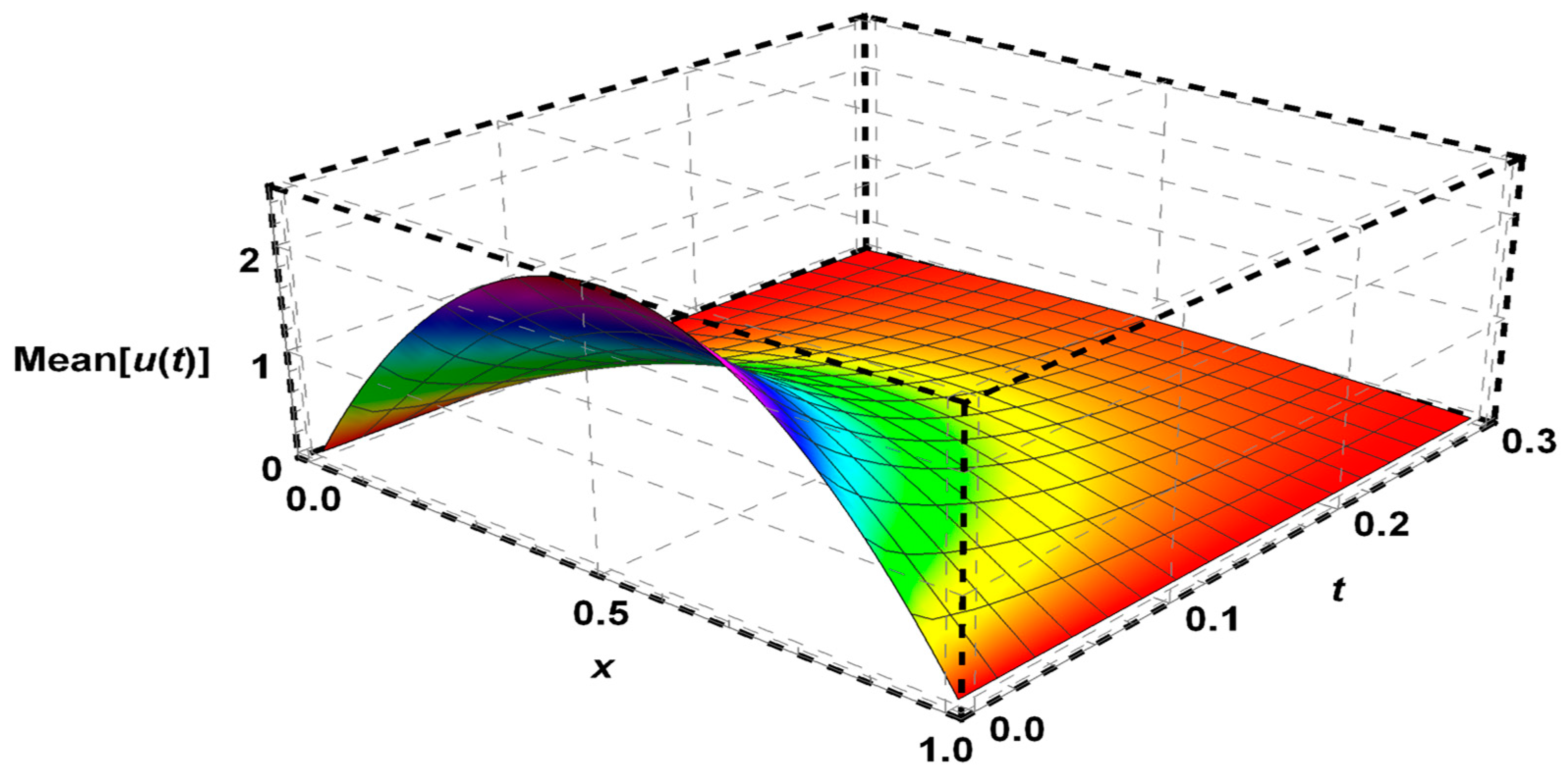
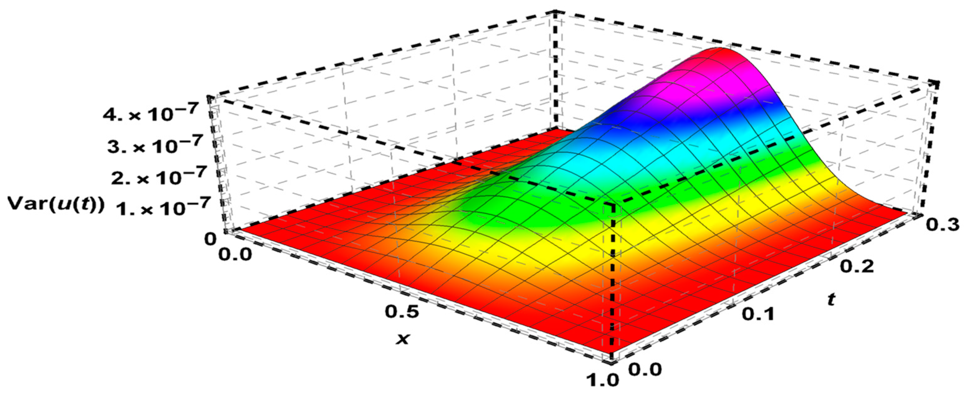
$$\mathcal{U}\left(x, 0\right)=x^2{\left(1-x\right)}^2, \mathcal{U}\left(0, t\right)=\mathcal{U}\left(1, t\right)=0, x\in \left[0, 1\right], t\in \left[0, 0.3\right]$$

The mean of solutions for Problem 3 is given by the proposed method in Table 3 and visualized in Figure 5. Also, an $O\left(h^7\right)$ variance of solutions is shown in Figure 6.

Problem 4. 

Consider the 1D SHE [6] is:

$${\mathcal{U}}_t\left(x, t\right)=\left({\displaystyle \frac{1}{{\pi }^2}}+\beta \dot{\mathbb{W}}\left(t\right)\right){\mathcal{U}}_{xx}\left(x, t\right)$$

(41)

$$\mathcal{U}\left(x, 0\right)=\sin \left(\pi x\right), \mathcal{U}\left(0, t\right)=\mathcal{U}\left(1, t\right)=0, x\in \left[0, 1\right], t\in \left[0, 1\right]$$

and its exact solution for $\beta =0$ is: $\mathcal{U}\left(x, t\right)=e^{-t}\mathit{sin} \left(\pi x\right)$.

For $\beta =0$, the FDFT method gave the solution of the deterministic heat equation in Problem 4 with an $O\left(h^6\right)$ absolute error as shown in

Table 5. The numerical results of Problem 4 for $\beta =0$ and $t=1$.

x	Exact	FDFT Method	Absolute Errors
$0.125$	$0.140781367$	$0.140780194$	$1.173\times {10}^{-6}$
$0.250$	$0.260130048$	$0.260127879$	$2.167\times {10}^{-6}$
$0.375$	$0.339876286$	$0.339873454$	$2.832\times {10}^{-6}$
$0.500$	$0.367879441$	$0.367876376$	$3.066\times {10}^{-6}$
$0.625$	$0.339876286$	$0.339873454$	$2.832\times {10}^{-6}$
$0.750$	$0.260130048$	$0.260127879$	$2.167\times {10}^{-6}$
$0.875$	$0.140781367$	$0.140780194$	$1.173\times {10}^{-6}$
$1.000$	$0.0$	$0.0$	$0.0$

and Figure 7. Furthermore, the mean and the variance of solutions are given in Table 4 and Figure 8 and Figure 9 for $\beta =0.01$.

Problem 5. 

Consider the 1D SHE [6] is:

$${\mathcal{U}}_t\left(x, t\right)=\left({\displaystyle \frac{1}{{2\pi }^2}}+\beta \dot{\mathbb{W}}\left(t\right)\right){\mathcal{U}}_{xx}\left(x, t\right)$$

(42)

$$\mathcal{U}\left(x, 0\right)=\sin \left(2\pi x\right), \mathcal{U}\left(0, t\right)=\mathcal{U}\left(1, t\right)=0, x\in \left[0, 1\right], t\in \left[0, 1\right]$$

and its exact solution for $\beta =0$ is: $\mathcal{U}\left(x, t\right)=e^{-2t}\mathit{sin} \left(2\pi x\right)$.

The present method obtained the solution of the deterministic heat equation in Problem 5 with an $O\left(h^6\right)$ absolute error as visualized in

Table 6. The numerical results of Problem 5 for $\beta =0$ and $t=1$.

x	Exact	FDFT Method	Absolute Errors
$0.125$	$0.095696497$	$0.095690119$	$6.377\times {10}^{-6}$
$0.250$	$0.135335283$	$0.135326265$	$9.018\times {10}^{-6}$
$0.375$	$0.09569649$	$0.095690119$	$6.377\times {10}^{-6}$
$0.500$	$0.0$	$0.0$	$0.0$
$0.625$	$-0.09569649$	$-0.095690119$	$6.377\times {10}^{-6}$
$0.750$	$-0.135335283$	$-0.135326265$	$9.018\times {10}^{-6}$
$0.875$	$-0.09569649$	$-0.095690119$	$6.377\times {10}^{-6}$
$1.000$	$0.0$	$0.0$	$0.0$

and Figure 10 for $\beta =0$, Furthermore, the mean of solutions for $\beta =0.02$ is shown in Figure 11.

In our study, the deterministic components exhibit a higher convergence rate compared to the stochastic components. This difference is attributed to the inherent complexity introduced by the stochastic term, which involves the Wiener process. For the deterministic part, the numerical method leverages the sixth-order CFD scheme, which ensures a high-order accuracy for smooth components of the solution. The convergence analysis confirms that the deterministic components converge with an expected order of $O\left(h^6\right)$.

In contrast, the stochastic component introduces randomness, which leads to increased variability and slower convergence. The discretization of the stochastic term relies on the Crank–Nicolson approach, combined with FDFT for efficient computation. The stochastic component is governed by the white noise and as noted in the simulations, converges at a rate consistent with $O\left(h^3\right)$, as influenced by the interplay between the noise and numerical scheme.

These differences are visually evident in Figure 2, Figure 4 and Figure 6, where the variance associated with the stochastic component is more prominent. This highlights the trade-off between the accuracy of deterministic and stochastic contributions, a factor intrinsic to solving stochastic differential equations.

6. Conclusions

In conclusion, compact finite difference (CFD) methods are widely employed to obtain the solution of various types of partial differential equations by discretizing them into systems of linear equations, which are typically solved through matrix inversion—a process that can be time-consuming, particularly for larger systems. This work introduces an innovative algorithm based on the sixth-order CFD approach, specifically designed for solving stochastic heat equations. By utilizing fast discrete Fourier transforms (FDFT) instead of traditional matrix inversion, our approach significantly enhances computational efficiency and effectiveness.

The importance of this method lies not only in its speed but also in its versatility, as the FDFT can be readily adapted for higher-dimensional problems. This capability opens new avenues for exploration, positioning our algorithm as a valuable tool in the numerical analysis of complex systems.

Looking ahead, we aim to extend our method to encompass fractional stochastic heat equations, which are vital for modelling processes exhibiting memory effects. Additionally, we plan to investigate its application within fuzzy environments, where uncertainty plays a critical role. These future directions will enhance the robustness and applicability of our method, further contributing to advancements in computational techniques for solving stochastic partial differential equations.

The fast discrete Fourier transform can be extended extend to solve the two-dimensional (2D) problems as follows:

Firstly, the 6th order CFD scheme of Equation (8) in 2D, are obtained:

$$2{\mathcal{U}}_{i-1,j}^{xx}+11{\mathcal{U}}_{i,j}^{xx}+2{\mathcal{U}}_{i+1,j}^{xx}={\displaystyle \frac{3}{4h_x^2}}\left({\mathcal{U}}_{i-2,j}+16{\mathcal{U}}_{i-1,j}-34{\mathcal{U}}_{i,j}+16{\mathcal{U}}_{i+1,j}+{\mathcal{U}}_{i+2,j}\right),$$

(43)

$$2{\mathcal{U}}_{i,j-1}^{yy}+11{\mathcal{U}}_{i,j}^{yy}+2{\mathcal{U}}_{i,j+1}^{yy}={\displaystyle \frac{3}{4h_y^2}}\left({\mathcal{U}}_{i,j-2}+16{\mathcal{U}}_{i,j-1}-34{\mathcal{U}}_{i,j}+16{\mathcal{U}}_{i,j+1}+{\mathcal{U}}_{i,j+2}\right).$$

(44)

Secondly, the 2D discrete sine transform for ${\mathcal{U}}_{ij}$ and its inverse for ${\widehat{\mathcal{U}}}_{pq}$ are defined as follows:

$${\mathcal{U}}_{ij}={\sum }_{p=1}^{M_x-1}{\sum }_{q=1}^{M_y-1}{\widehat{\mathcal{U}}}_{pq}\sin \left({\displaystyle \frac{\pi \left(i\right)p}{M_x}}\right)\sin \left({\displaystyle \frac{\pi \left(j\right)q}{M_y}}\right),$$

(45)

$${\widehat{\mathcal{U}}}_{pq}={\displaystyle \frac{2}{M_x}}{\displaystyle \frac{2}{M_y}}{\sum }_{i=1}^{M_x-1}{\sum }_{j=1}^{M_y-1}{\mathcal{U}}_{ij}\sin \left({\displaystyle \frac{\pi \left(i\right)p}{M_x}}\right)\sin \left({\displaystyle \frac{\pi \left(j\right)q}{M_y}}\right).$$

(46)

Applying (45) to Equation (43) leads to

$$\begin{array}{c}2\sum _{p=1}^{M_x-1}\sum _{q=1}^{M_y-1}{\widehat{\mathcal{U}}}_{pq}^{xx}\sin \left({\displaystyle \frac{\pi \left(i-1\right)p}{M_x}}\right)\sin \left({\displaystyle \frac{\pi \left(j\right)q}{M_y}}\right)+\\ 11\sum _{p=1}^{M_x-1}\sum _{q=1}^{M_y-1}{\widehat{\mathcal{U}}}_{pq}^{xx}\sin \left({\displaystyle \frac{\pi \left(i\right)p}{M_x}}\right)\sin \left({\displaystyle \frac{\pi \left(j\right)q}{M_y}}\right)+\\ 2\sum _{p=1}^{M_x-1}\sum _{q=1}^{M_y-1}{\widehat{\mathcal{U}}}_{pq}^{xx}\sin \left({\displaystyle \frac{\pi \left(i+1\right)p}{M_x}}\right)\sin \left({\displaystyle \frac{\pi \left(j\right)q}{M_y}}\right)=\\ {\displaystyle \frac{3}{4h_x^2}}[\sum _{p=1}^{M_x-1}\sum _{q=1}^{M_y-1}{\widehat{\mathcal{U}}}_{pq}\sin \left({\displaystyle \frac{\pi \left(i-2\right)p}{M_x}}\right)\sin \left({\displaystyle \frac{\pi \left(j\right)q}{M_y}}\right)+\\ 16\sum _{p=1}^{M_x-1}\sum _{q=1}^{M_y-1}{\widehat{\mathcal{U}}}_{pq}\sin \left({\displaystyle \frac{\pi \left(i-1\right)p}{M_x}}\right)\sin \left({\displaystyle \frac{\pi \left(j\right)q}{M_y}}\right)-\\ 34\sum _{p=1}^{M_x-1}\sum _{q=1}^{M_y-1}{\widehat{\mathcal{U}}}_{pq}\sin \left({\displaystyle \frac{\pi \left(i\right)p}{M_x}}\right)\sin \left({\displaystyle \frac{\pi \left(j\right)q}{M_y}}\right)+\\ 16\sum _{p=1}^{M_x-1}\sum _{q=1}^{M_y-1}{\widehat{\mathcal{U}}}_{pq}\sin \left({\displaystyle \frac{\pi \left(i+1\right)p}{M_x}}\right)\sin \left({\displaystyle \frac{\pi \left(j\right)q}{M_y}}\right)+\\ \sum _{p=1}^{M_x-1}\sum _{q=1}^{M_y-1}{\widehat{\mathcal{U}}}_{pq}\sin \left({\displaystyle \frac{\pi \left(i+2\right)p}{M_x}}\right)\sin \left({\displaystyle \frac{\pi \left(j\right)q}{M_y}}\right)],\end{array}$$

$$\begin{array}{c}\sum _{p=1}^{M_x-1}\sum _{q=1}^{M_y-1}{\widehat{\mathcal{U}}}_{pq}^{xx}[2\sin \left({\displaystyle \frac{\pi \left(i-1\right)p}{M_x}}\right)+11\sin \left({\displaystyle \frac{\pi \left(i\right)p}{M_x}}\right)\\ +2\sin \left({\displaystyle \frac{\pi \left(i+1\right)p}{M_x}}\right)]\sin \left({\displaystyle \frac{\pi \left(j\right)q}{M_y}}\right)= {\displaystyle \frac{3}{4h_x^2}}\sum _{p=1}^{M_x-1}\sum _{q=1}^{M_y-1}{\widehat{\mathcal{U}}}_{pq}[\sin \left({\displaystyle \frac{\pi \left(i-2\right)p}{M_x}}\right)+\\ 16\sin \left({\displaystyle \frac{\pi \left(i-1\right)p}{M_x}}\right)-34\sin \left({\displaystyle \frac{\pi \left(i\right)p}{M_x}}\right)+16\sin \left({\displaystyle \frac{\pi \left(i+1\right)p}{M_x}}\right)+\sin \left({\displaystyle \frac{\pi \left(i+2\right)p}{M_x}}\right)]\sin \left({\displaystyle \frac{\pi \left(j\right)q}{M_y}}\right),\end{array}$$

After simplifications,

$$\left[4\cos \left({\displaystyle \frac{p\pi }{M_x}}\right)+11\right]{\widehat{\mathcal{U}}}_{pq}^{xx}={\displaystyle \frac{3}{2h_x^2}}\left[\cos \left({\displaystyle \frac{2p\pi }{M_x}}\right)+16\cos \left({\displaystyle \frac{p\pi }{M_x}}\right)-17\right]{\widehat{\mathcal{U}}}_{pq},$$

Hence,

$${\widehat{\mathcal{U}}}_{pq}^{xx}={\displaystyle \frac{3}{2h_x^2}}\left[{\displaystyle \frac{\cos \left(\frac{2p\pi }{M_x}\right)+16\cos \left(\frac{p\pi }{M_x}\right)-17}{4\cos \left(\frac{p\pi }{M_x}\right)+11}}\right]{\widehat{\mathcal{U}}}_{pq},$$

(47)

Similarly, applying (45) to Equation (44) and after simplifications, we have

$${\widehat{\mathcal{U}}}_{pq}^{yy}={\displaystyle \frac{3}{2h_y^2}}\left[{\displaystyle \frac{\cos \left(\frac{2q\pi }{M_y}\right)+16\cos \left(\frac{q\pi }{M_y}\right)-17}{4\cos \left(\frac{q\pi }{M_y}\right)+11}}\right]{\widehat{\mathcal{U}}}_{pq}.$$

(48)

Also, the fast discrete Fourier transform can be extended extend to solve the three-dimensional (3D) problems as follows:

Firstly, the 6th order CFD scheme of Equation (8) in 3D, are obtained:

$$2{\mathcal{U}}_{i-1,j,k}^{xx}+11{\mathcal{U}}_{i,j,k}^{xx}+2{\mathcal{U}}_{i+1,j,k}^{xx}={\displaystyle \frac{3}{4h_x^2}}\left({\mathcal{U}}_{i-2,j,k}+16{\mathcal{U}}_{i-1,j,k}-34{\mathcal{U}}_{i,j,k}+16{\mathcal{U}}_{i+1,j,k}+{\mathcal{U}}_{i+2,j,k}\right),$$

(49)

$$2{\mathcal{U}}_{i-1,j,k}^{yy}+11{\mathcal{U}}_{i,j,k}^{yy}+2{\mathcal{U}}_{i+1,j,k}^{yy}={\displaystyle \frac{3}{4h_x^2}}\left({\mathcal{U}}_{i-2,j,k}+16{\mathcal{U}}_{i-1,j,k}-34{\mathcal{U}}_{i,j,k}+16{\mathcal{U}}_{i+1,j,k}+{\mathcal{U}}_{i+2,j,k}\right),$$

(50)

$$2{\mathcal{U}}_{i-1,j,k}^{zz}+11{\mathcal{U}}_{i,j,k}^{zz}+2{\mathcal{U}}_{i+1,j,k}^{zz}={\displaystyle \frac{3}{4h_x^2}}\left({\mathcal{U}}_{i-2,j,k}+16{\mathcal{U}}_{i-1,j,k}-34{\mathcal{U}}_{i,j,k}+16{\mathcal{U}}_{i+1,j,k}+{\mathcal{U}}_{i+2,j,k}\right),$$

(51)

Secondly, the 3D discrete sine transform for ${\mathcal{U}}_{ijk}$ and its inverse for ${\widehat{\mathcal{U}}}_{pql}$are defined as follows:

$${\mathcal{U}}_{ijk}={\sum }_{p=1}^{M_x-1}{\sum }_{q=1}^{M_y-1}{\sum }_{l=1}^{M_z-1}{\widehat{\mathcal{U}}}_{pql}\sin \left({\displaystyle \frac{\pi \left(i\right)p}{M_x}}\right)\sin \left({\displaystyle \frac{\pi \left(j\right)q}{M_y}}\right)\sin \left({\displaystyle \frac{\pi \left(k\right)l}{M_z}}\right),$$

(52)

$${\widehat{\mathcal{U}}}_{pql}={\displaystyle \frac{2}{M_x}}{\displaystyle \frac{2}{M_y}}{\displaystyle \frac{2}{M_z}}{\sum }_{p=1}^{M_x-1}{\sum }_{q=1}^{M_y-1}{\sum }_{l=1}^{M_z-1}{\mathcal{U}}_{ijk}\sin \left({\displaystyle \frac{\pi \left(i\right)p}{M_x}}\right)\sin \left({\displaystyle \frac{\pi \left(j\right)q}{M_y}}\right)\sin \left({\displaystyle \frac{\pi \left(k\right)l}{M_z}}\right),$$

(53)

Applying (52) to Equations (49)– (51), and after simplifications, we obtain

$${\widehat{\mathcal{U}}}_{pql}^{xx}={\displaystyle \frac{3}{2h_x^2}}\left[{\displaystyle \frac{\cos \left(\frac{2p\pi }{M_x}\right)+16\cos \left(\frac{p\pi }{M_x}\right)-17}{4\cos \left(\frac{p\pi }{M_x}\right)+11}}\right]{\widehat{\mathcal{U}}}_{pql},$$

(54)

$${\widehat{\mathcal{U}}}_{pql}^{yy}={\displaystyle \frac{3}{2h_y^2}}\left[{\displaystyle \frac{\cos \left(\frac{2q\pi }{M_y}\right)+16\cos \left(\frac{q\pi }{M_y}\right)-17}{4\cos \left(\frac{q\pi }{M_y}\right)+11}}\right]{\widehat{\mathcal{U}}}_{pql},$$

(55)

$${\widehat{\mathcal{U}}}_{pql}^{zz}={\displaystyle \frac{3}{2h_y^2}}\left[{\displaystyle \frac{\cos \left(\frac{2l\pi }{M_z}\right)+16\cos \left(\frac{l\pi }{M_z}\right)-17}{4\cos \left(\frac{l\pi }{M_z}\right)+11}}\right]{\widehat{\mathcal{U}}}_{pql}$$

(56)

References

- Hassan Khabir, M. Cubic B-spline Collocation Method for One-Dimensional Heat Equation. Pure Appl. Math. J. 2017, 6, 51. [Google Scholar] [CrossRef]
- Iqbal, M.; Zainuddin, N.; Daud, H.; Kanan, R.; Jusoh, R.; Ullah, A.; Khan, I.K. Numerical Solution of Heat Equation using Modified Cubic B-spline Collocation Method. J. Adv. Res. Numer. Heat Transf. 2024, 20, 23–35. [Google Scholar] [CrossRef]
- Da Prato, G.Z.J. Stochastic Equations in Infinite Dimensions, 2nd ed.; Cambridge University Press: Cambridge, UK, 2014. [Google Scholar]
- Hammad, D.A.; Semary, M.S.; Khattab, A.G. Ten non-polynomial cubic splines for some classes of Fredholm integral equations. Ain Shams Eng. J. 2022, 13, 101666. [Google Scholar] [CrossRef]
- Fareed, A.F.; Khattab, A.G.; Semary, M.S. A novel stochastic ten non-polynomial cubic splines method for heat equations with noise term. Partial Differ. Equ. Appl. Math. 2024, 10, 100677. [Google Scholar] [CrossRef]
- Heydari, M.H.; Hooshmandasl, M.R.; Barid Loghmani, G.; Cattani, C. Wavelets Galerkin method for solving stochastic heat equation. Int. J. Comput. Math. 2016, 93, 1579–1596. [Google Scholar] [CrossRef]
- Uma, D.; Jafari, H.; Raja Balachandar, S.; Venkatesh, S.G. An Approximation Method for Stochastic Heat Equation Driven by White Noise. Int. J. Appl. Comput. Math. 2022, 8, 274. [Google Scholar] [CrossRef]
- Anton, R.; Cohen, D.; Quer-Sardanyons, L. A fully discrete approximation of the one-dimensional stochastic heat equation. IMA J. Numer. Anal. 2020, 40, 247–284. [Google Scholar] [CrossRef]
- Fareed, A.F.; Semary, M.S.; Hassan, H.N. Two semi-analytical approaches to approximate the solution of stochastic ordinary differential equations with two enormous engineering applications. Alex. Eng. J. 2022, 61, 11935–11945. [Google Scholar] [CrossRef]
- Nouy, A. Recent developments in spectral stochastic methods for the numerical solution of stochastic partial differential equations. Arch. Comput. Methods Eng. 2009, 16, 251–285. [Google Scholar] [CrossRef]
- Moghaddam, B.P.; Mostaghim, Z.S.; Pantelous, A.A.; Machado, J.A.T. An integro quadratic spline-based scheme for solving nonlinear fractional stochastic differential equations with constant time delay. Commun. Nonlinear Sci. Numer. Simul. 2021, 92, 105475. [Google Scholar] [CrossRef]
- Hamed, M.; El-Twail, M.A.; El-Desouky, B.; El-Beltagy, M.A. Solution of Nonlinear Stochastic Langevin’s Equation Using WHEP, Pickard and HPM Methods. Appl. Math. 2014, 5, 398–412. [Google Scholar] [CrossRef]
- El-Tawil, M.A.; Fareed, A.F. Solution of Stochastic Cubic and Quintic Nonlinear Diffusion Equation Using WHEP, Pickard and HPM Methods. Open J. Discret. Math. 2011, 1, 6–21. [Google Scholar] [CrossRef]
- Gerencsér, M.; Gyöngy, I. Finite Difference Schemes for Stochastic Partial Differential Equations in Sobolev Spaces. Appl. Math. Optim. 2015, 72, 77–100. [Google Scholar] [CrossRef]
- Boulakia, M.; Genadot, A.; Thieullen, M. Simulation of SPDEs for Excitable Media Using Finite Elements. J. Sci. Comput. 2015, 65, 171–195. [Google Scholar] [CrossRef]
- Youssri, Y.H.; Muttardi, M.M. A Mingled Tau-Finite Difference Method for Stochastic First-Order Partial Differential Equations. Int. J. Appl. Comput. Math. 2023, 9, 14. [Google Scholar] [CrossRef]
- Babaei, A.; Jafari, H.; Banihashemi, S. A collocation approach for solving time-fractional stochastic heat equation driven by an additive noise. Symmetry 2020, 12, 904. [Google Scholar] [CrossRef]
- Masti, I.; Sayevand, K. On collocation-Galerkin method and fractional B-spline functions for a class of stochastic fractional integro-differential equations. Math. Comput. Simul. 2024, 216, 263–287. [Google Scholar] [CrossRef]
- Hammad, D.A.; El-Azab, M.S. A 2N order compact finite difference method for solving the generalized regularized long wave (GRLW) equation. Appl. Math. Comput. 2015, 253, 248–261. [Google Scholar] [CrossRef]
- Hammad, D.A.; El-Azab, M.S. 2N order compact finite difference scheme with collocation method for solving the generalized Burger’s-Huxley and Burger’s-Fisher equations. Appl. Math. Comput. 2015, 258, 296–311. [Google Scholar] [CrossRef]
- Biazar, J.; Asayesh, R. An efficient high-order compact finite difference method for the Helmholtz equation. Comput. Methods Differ. Equ. 2020, 8, 553–563. [Google Scholar] [CrossRef]
- Wang, H.; Zhang, Y.; Ma, X.; Qiu, J.; Liang, Y. An efficient implementation of fourth-order compact finite difference scheme for Poisson equation with Dirichlet boundary conditions. Comput. Math. Appl. 2016, 71, 1843–1860. [Google Scholar] [CrossRef]
- Hosseinverdi, S.; Fasel, H.F. A fourth-order accurate compact difference scheme for solving the three-dimensional poisson equation with arbitrary boundaries. In AIAA Scitech 2020 Forum; American Institute of Aeronautics and Astronautics Inc., AIAA: Reston, VA, USA, 2020; Volume 1, Part F. [Google Scholar] [CrossRef]
- Gatiso, A.H.; Belachew, M.T.; Wolle, G.A. Sixth-order compact finite difference scheme with discrete sine transform for solving Poisson equations with Dirichlet boundary conditions. Results Appl. Math. 2021, 10, 100148. [Google Scholar] [CrossRef]
- Liao, F.; Zhang, L.-M. High accuracy split-step finite difference method for Schrödinger-KdV equations. Commun. Theor. Phys. 2018, 70, 413. [Google Scholar] [CrossRef]
- Särkkä, S.; Solin, A. Applied Stochastic Differential Equations; Cambridge University Press: Cambridge, UK, 2019. [Google Scholar] [CrossRef]
- Hammad, D.A.; Semary, M.S.; Khattab, A.G. Parametric quintic spline for time fractional Burger’s and coupled Burgers’ equations. Fixed Point Theory Algorithms Sci. Eng. 2023, 2023, 9. [Google Scholar] [CrossRef]
- Fang, L.; Ma, L.; Ding, S.; Zhao, D. Finite-time stabilization for a class of high-order stochastic nonlinear systems with an output constraint. Appl. Math. Comput. 2019, 358, 63–79. [Google Scholar] [CrossRef]
- Chen, W.; Fu, Z.; Grafakos, L.; Wu, Y. Fractional Fourier transforms on Lp and applications. Appl. Comput. Harmon. Anal. 2021, 55, 71–96. [Google Scholar] [CrossRef]
- Yang, Y.; Wu, Q.; Jhang, S.T.; Kang, Q. Approximation Theorems Associated with Multidimensional Fractional Fourier Transform and Applications in Laplace and Heat Equations. Fractal Fract. 2022, 6, 625. [Google Scholar] [CrossRef]
- Roozbahani, M.M.; Aminikhah, H.; Tahmasebi, M. Numerical multi-scaling method to solve the linear stochastic partial differential equations. Comput. Appl. Math. 2018, 37, 5527–5541. [Google Scholar] [CrossRef]