An Improved King–Werner-Type Method Based on Cubic Interpolation: Convergence Analysis and Complex Dynamics

Abstract

In this paper, we study the convergence and complex dynamics of a novel higher-order multipoint iteration scheme to solve nonlinear equations. The approach is based upon utilizing cubic interpolation in the second step of the King–Werner method to improve its convergence order from $2.414$ to 3 and the efficiency index from $1.554$ to $1.732$, which is higher than the efficiency of optimal fourth- and eighth-order iterative schemes. The proposed method is validated through numerical and dynamic experiments concerning the absolute error, approximated computational order, regions of convergence, and CPU time (sec) on the real-world problems, including Kepler’s equation, isentropic supersonic flow, and law of population growth, demonstrating superior performance compared to some existing well-known methods. Commonly, regions of convergence of iterative methods are investigated and compared by plotting attractor basins of iteration schemes in the complex plane on polynomial functions of the type $z^n-1$. However, in this paper, the attractor basins of the proposed method are investigated on diverse nonlinear functions. The proposed scheme creates portraits of basins of attraction faster with wider convergence areas outperforming existing well-known iteration schemes.

1. Introduction

Solving nonlinear equations of the form $f\left(x\right)=0,$ where $f:I\in \mathbb{R}\to \mathbb{R}$ is a continuously differentiable function defined on an open interval I, is a fundamental yet challenging problem encountered across various disciplines of science and engineering. In many practical applications, such equations do not admit closed-form analytical solutions, necessitating the use of iterative numerical techniques to approximate the roots with a desired level of accuracy.

Among these techniques, Newton’s method [1] remains one of the most widely used due to its quadratic convergence and simplicity, particularly when the function f and its derivative $f^{\prime }$ are easy to compute. Newton’s method is a classical iterative technique, which starts with an initial approximation $x_0$ and generates a sequence $x_n$ from the following relation:

$$x_{n+1}=x_n-{\displaystyle \frac{f\left(x_n\right)}{f^{\prime }\left(x_n\right)}}.$$

(1)

Multipoint methods overcome the theoretical limits of any one-point method like Newton’s method (1) regarding the order of convergence and informational and computational efficiency [2]. Thus, they are of greater practical importance than one-point methods. A comprehensive study of multipoint iterative methods for simple roots can be found in [2,3,4]. To expedite the convergence of Newton’s method, many third-order two-point methods, requiring the evaluations of either the first derivative or first and second derivatives, have also been proposed (see [1,2,5,6,7,8,9]).

Kung and Traub [10] conjectured that an optimal method of order n is a method without memory which requires $n+1$ function evaluations per iteration. To satisfy this conjecture, several optimal fourth and eighth-order methods have been derived and investigated in the last few years (for example, see [4,11,12,13,14,15,16,17,18,19,20]).

Efficiency index of an iteration scheme (IS) is computed using a well-known formula due to Ostrowski [1] given by:

$$E\left(IS\right)=p^{{\displaystyle \frac{1}{\eta }}},$$

(2)

where p indicates order convergence of $\left(IS\right)$ and $\eta$ is the total number of evaluations of functions used by an iterative scheme per iterative cycle. For instance, the efficiency of Newton’s method is $E\left(3\right)={\left(2\right)}^{{\displaystyle \frac{1}{2}}}\approx 1.414$. Please note that an optimal fourth-order scheme, for example, the well-known King method [21] has an efficiency index, $4^{{\displaystyle \frac{1}{3}}}\simeq 1.587$. However, the new method designed in this paper has higher computational efficiency, i.e., $1.732$.

The main motivation of this work is to improve the convergence order and efficiency of the well-known King–Werner method [22] by introducing cubic interpolation in its second step. This enhancement raises the order of convergence from $2.414$ to 3 and the efficiency index from $1.554$ to $1.732$, outperforming many existing optimal fourth- and eighth-order schemes in practice. Our aim is to present a more effective and computationally competitive alternative iterative scheme for solving nonlinear equations.

To this end, we propose a novel third-order multipoint iterative method and analyze its convergence analysis as well as complex dynamics. The method is validated through several numerical and graphical experiments, demonstrating both robustness and superior performance. The iteration method derived in this paper is more efficient than the optimal methods described above. Moreover, higher-order convergent techniques free from the evaluation of derivatives, for instance, the schemes presented in the papers [23,24], are of specific significance since a large number of nonlinear equations involve a non-differentiable term.

We consider the derivative-free King–Werner method given as follows [22]:

$$\begin{array}{cc}\hfill z_{n+1}& =x_n-{\displaystyle \frac{f\left(x_n\right)}{[x_n,z_n;f]}},\hfill \\ \hfill x_{n+1}& =z_{n+1}-{\displaystyle \frac{f\left(z_{n+1}\right)}{[x_n,z_n;f]}},n=0,1,2,\dots ,\hfill \end{array}$$

(3)

where $x_0,z_0$ are initial points and $[x_n,z_n;f]$ is first order divided difference. We improve the convergence order of the King–Werner method (3) from $2.414$ to 3 under the same hypothesis.

The contents of the paper are summarized below. The development of the new method is presented in Section 2. In Section 3, the convergence analysis of the new method is investigated. Numerical examples, including some real-world applications, are considered for the verification of theoretical results and the comparison with some existing methods in Section 4. Section 5 presents the complex dynamics and stability analysis of the new method compared with some existing well-known methods using basins of attraction. Finally, the summary of the key findings is concluded in Section 6.

2. The Method

We define a two-step iterative scheme given by:

$$\begin{array}{cc}\hfill z_{n+1}& =x_n-{\displaystyle \frac{f\left(x_n\right)}{[x_n,z_n;f]}},\hfill \\ \hfill x_{n+1}& =z_{n+1}-{\displaystyle \frac{f\left(z_{n+1}\right)}{C^{\prime }\left(z_{n+1}\right)}},\hfill \end{array}$$

(4)

where C is a cubic curve interpolation given by,

$$C\left(t\right)=a{(t-x_n)}^3+b{(t-x_n)}^2+c(t-x_n)+d,$$

(5)

employing the following conditions:

$$C\left(x_n\right)=f\left(x_n\right),C\left(z_n\right)=f\left(z_n\right)\mathrm{and}C\left(z_{n+1}\right)=f\left(z_{n+1}\right).$$

(6)

Now, for the coefficients b, c and d in terms of the coefficient a by applying the conditions (6) in R(t), then

$$\begin{array}{cc}\hfill b& ={\displaystyle \frac{{\delta }_1-{\delta }_2}{{\lambda }_1-{\lambda }_2}}+a({\lambda }_1+{\lambda }_2),\hfill \end{array}$$

(7)

$$\begin{array}{cc}\hfill c& ={\displaystyle \frac{{\delta }_2{\lambda }_1-{\delta }_1{\lambda }_2}{{\lambda }_1-{\lambda }_2}}+a{\lambda }_1{\lambda }_2,\hfill \end{array}$$

(8)

$$\begin{array}{cc}\hfill d& =f\left(x_n\right),\hfill \end{array}$$

(9)

where,

$$\begin{array}{cc}\hfill {\lambda }_1& =z_n-x_k,{\lambda }_2=z_{n+1}-x_n,\hfill \\ \hfill {\delta }_1& ={\displaystyle \frac{f\left(z_n\right)-f\left(x_n\right)}{z_n-x_n}},{\delta }_2={\displaystyle \frac{f\left(z_{k+1}\right)-f\left(x_n\right)}{z_{n+1}-x_n}}.\hfill \end{array}$$

Simple calculations yield:

$$C^{\prime }\left(z_{n+1}\right)=3a{(z_{n+1}-x_n)}^2+2b(z_{n+1}-x_n)+c={\displaystyle \frac{{\delta }_2({\lambda }_1-2{\lambda }_2)+{\delta }_1{\lambda }_2-a{({\lambda }_1-{\lambda }_2)}^2{\lambda }_2}{{\lambda }_1-{\lambda }_2}}.$$

(10)

Hence, by using Equation (10), the iteration scheme (4) yields:

$$\begin{array}{cc}\hfill z_{n+1}& =x_n-{\displaystyle \frac{f\left(x_n\right)}{[x_n,z_n;f]}},\hfill \\ \hfill x_{n+1}& =z_{n+1}-{\displaystyle \frac{{\lambda }_1-{\lambda }_2}{{\delta }_2({\lambda }_1-2{\lambda }_2)+{\delta }_1{\lambda }_2-a{({\lambda }_1-{\lambda }_2)}^2{\lambda }_2}}f\left(z_{n+1}\right).\hfill \end{array}$$

(11)

The iterative scheme (11) includes a free parameter a, which plays a crucial role in enhancing the behavior and performance of the proposed method. By varying the value of a, different iterative methods can be derived from the same general formulation. This flexibility allows for tuning the method to achieve optimal convergence characteristics under different problem conditions. In this manuscript, however, we focus on a specific case by selecting a fixed value of a, namely $a=1$. The convergence analysis of the iteration scheme (11) is investigated in the next section.

3. Convergence

To study the convergence analysis of the method (11), we take into account the idea of R- order of convergence presented by Ortega-Rheinboldt [25]. Let $x_n$ be a sequence of approximations, generated by an iteration method, which converges to a zero $\alpha$ of $f\left(x\right)=0$ with the R-order of convergence, $O_R\ge r$, then we can write:

$$e_{n+1}\sim e_n^r,$$

(12)

where $e_{n+1}=x_n-\alpha$ is the error at the $n+1$-th iteration.

Let $e_n=x_n-\alpha ,$${\overline{e}}_n=z_n-\alpha$, be the errors in the n-th iteration of an iteration scheme. With the help of Taylor’s expansions of $f\left(x_n\right)$ and $f\left(z_n\right)$ about $\alpha$ and considering that $f\left(\alpha \right)=0$ and $f^{\prime }\left(\alpha \right)\ne 0,$ we have,

$$f\left(x_n\right)=f^{\prime }\left(\alpha \right)[e_n+A_2{e}_n^2+A_3{e}_n^3+O\left(e_n^4\right)],$$

(13)

$$f\left(z_n\right)=f^{\prime }\left(\alpha \right)[{\overline{e}}_n+A_2{\overline{e}}_n^2+A_3{\overline{e}}_n^3+O\left({\overline{e}}_n^4\right)],$$

(14)

where $A_i=(1/i!)f^{\left(i\right)}\left(\alpha \right)/f^{\prime }\left(\alpha \right),i>1.$

• By using the expressions (13) and (14) in the first step of (11), we obtain

  $${\overline{e}}_{n+1}=A_2{\overline{e}}_n{e}_n+(A_3-A_2^2)({\overline{e}}_n^2{e}_n+{\overline{e}}_n{e}_n^2)+\dots .$$

  (15)

  Again, by using (13), (14) and (15) in the scheme (11), we obtain:

  $$e_{n+1}=\left(A_2(A_2^2-A_3+{\displaystyle \frac{a}{f^{\prime }\left(\alpha \right)}})\right){\overline{e}}_n^2{e}_n^2+\dots .$$

  (16)

  The above error relations are essential to prove the following result.

Theorem 1.

Let $x_0$ be an initial guess sufficiently close to a zero α of f, then the iteration scheme (11) has R-order of convergence at least 3.

Proof. 

The Equations (15) and (16) yield, respectively:

$${\overline{e}}_{n+1}\sim {\overline{e}}_n{e}_n$$

(17)

and

$$e_{n+1}\sim {\overline{e}}_n^2{e}_n^2.$$

(18)

Consequently,

$$e_{n+1}\sim {\left({\overline{e}}_{n+1}\right)}^2.$$

(19)

Suppose that the sequences $\left\{x_n\right\}$ and $\left\{y_n\right\}$ have R-order of convergence r and p, respectively. Then, the Equation (12) yields:

$$e_{n+1}\sim e_n^r$$

(20)

and

$${\overline{e}}_{n+1}\sim {\overline{e}}_n^p.$$

(21)

By combining (19) and (20), we obtain:

$${\overline{e}}_{n+1}\sim e_n^{{\displaystyle \frac{r}{2}}}.$$

(22)

Also, by combining (21) and (22), we obtain:

$${\overline{e}}_n\sim e_n^{{\displaystyle \frac{r}{2p}}}.$$

(23)

Now, from Equations (18) and (23), we obtain:

$$e_{n+1}\sim e_n^2{e}_n^{{\displaystyle \frac{r}{p}}}\sim e_n^{2+{\displaystyle \frac{r}{p}}}.$$

(24)

From (23), we obtain:

$${\overline{e}}_{n+1}\sim e_{n+1}^{{\displaystyle \frac{r}{2p}}},i.e.e_{n+1}\sim {\overline{e}}_{n+1}^{{\displaystyle \frac{2p}{r}}}.$$

(25)

By comparing the pairs of expressions, (20) ∧ (24) and (19) ∧ (25), we obtain:

$$\begin{array}{c}\hfill 2+{\displaystyle \frac{r}{p}}=r,\\ \hfill {\displaystyle \frac{2p}{r}}=2.\end{array}$$

The solution to the above equations yields $r=3$ and $p=3$, indicating that the new method (11) has third order of convergence. Hence the result. □

4. Numerical Results and Comparison

This section evaluates the efficacy and validity of the proposed method (11) by employing Mathematica 11 programming environment with arbitrary-precision arithmetic. For the sake of comparison, we consider second order methods of Newton [25] and Steffensen [26]; third-order methods by Özban [8], Weerakoon-Fernando [9], Halley [7], Ostrowski [1] and the method given by (3). These methods are given as follows:

• Newton’s method:

  $$x_{n+1}=x_n-{\displaystyle \frac{f\left(x_n\right)}{f^{\prime }\left(x_n\right)}}.$$

  (26)

  Steffensen’s method:

  $$\begin{array}{cc}\hfill z_n& =x_n+f\left(x_n\right),\hfill \\ \hfill x_{n+1}& =x_n-{\displaystyle \frac{f\left(x_n\right)}{[z_n,x_n;f]}}.\hfill \end{array}$$

  (27)

  Özban’s method:

  $$\begin{array}{cc}\hfill z_{n+1}& =x_n-{\displaystyle \frac{f\left(x_n\right)}{f^{\prime }\left(x_n\right)}},\hfill \\ \hfill x_{n+1}& =x_n-{\displaystyle \frac{f\left(x_n\right)}{f^{\prime }((x_n+z_{n+1})/2)}}.\hfill \end{array}$$

  (28)

  Weerakoon-Fernando’s method:

  $$\begin{array}{cc}\hfill z_{n+1}& =x_n-{\displaystyle \frac{f\left(x_n\right)}{f^{\prime }\left(x_n\right)}},\hfill \\ \hfill x_{n+1}& =x_n-{\displaystyle \frac{2f\left(x_n\right)}{f^{\prime }\left(x_n\right)+f^{\prime }\left(z_{n+1}\right)}}.\hfill \end{array}$$

  (29)

  Halley’s method:

  $$x_{n+1}=x_n-{\displaystyle \frac{2f\left(x_n\right)f^{\prime }\left(x_n\right)}{2f^{\prime }{\left(x_n\right)}^2-f\left(x_n\right)f^{\prime \prime }\left(x_n\right)}}.$$

  (30)

  Ostrowski’s method:

  $$x_{n+1}=x_n-{\displaystyle \frac{f\left(x_n\right)}{\sqrt{f^{\prime }{\left(x_n\right)}^2-f\left(x_n\right)f^{\prime \prime }\left(x_n\right)}}}.$$

  (31)

Numerical results displayed in

Table 1. Comparison of different iteration methods on $f_1\left(x\right)$, taking $x_0=0.5$.

Method	n	$|{\mathit{x}}_2-{\mathit{x}}_1|$	$|{\mathit{x}}_3-{\mathit{x}}_2|$	$|{\mathit{x}}_4-{\mathit{x}}_3|$	ACOC
Newton	7	$7.916(-3)$	$1.437(-6)$	$4.560(-14)$	2.000
Steffensen	7	$1.667(-2)$	$1.198(-5)$	$5.546(-12)$	2.000
Method (3) $(z_0=0.1)$	5	$6.649(-6)$	$7.573(-16)$	$1.832(-39)$	2.414
Özban	5	$4.903(-4)$	$1.561(-12)$	$5.034(-38)$	3.000
Weerakoon	5	$1.335(-3)$	$6.648(-11)$	$8.207(-33)$	3.000
Halley	5	$2.250(-3)$	$6.206(-10)$	$1.300(-29)$	3.000
Ostrowski	5	$2.399(-3)$	$7.547(-10)$	$2.349(-29)$	3.000
Method (11) $(z_0=0.1)$	4	$7.490(-6)$	$3.645(-19)$	$2.357(-59)$	3.000

,

Table 2. Comparison of different iteration methods on $f_2\left(x\right)$, taking $x_0=1.4$.

Method	n	$|{\mathit{x}}_2-{\mathit{x}}_1|$	$|{\mathit{x}}_3-{\mathit{x}}_2|$	$|{\mathit{x}}_4-{\mathit{x}}_3|$	ACOC
Newton	7	$7.463(-3)$	$5.958(-6)$	$3.756(-12)$	2.000
Steffensen	8	$4.138(-2)$	$2.899(-4)$	$1.334(-8)$	2.000
Method (3) $(z_0=1.7)$	5	$4.347(-5)$	$1.510(-12)$	$1.082(-30)$	2.414
Özban	5	$3.903(-3)$	$1.842(-9)$	$1.936(-28)$	3.000
Weerakoon	5	$8.875(-3)$	$1.925(-8)$	$2.022(-25)$	3.000
Halley	5	$2.448(-2)$	$1.392(-6)$	$2.434(-19)$	3.000
Ostrowski	5	$2.342(-2)$	$1.152(-6)$	$1.296(-19)$	3.000
Method (11) $(z_0=1.7)$	5	$2.025(-4)$	$2.745(-14)$	$2.313(-43)$	3.000

,

Table 3. Comparison of different iteration methods on $f_3\left(x\right)$, taking $x_0=0.5$.

Method	n	$|{\mathit{x}}_2-{\mathit{x}}_1|$	$|{\mathit{x}}_3-{\mathit{x}}_2|$	$|{\mathit{x}}_4-{\mathit{x}}_3|$	ACOC
Newton	8	$6.480(-2)$	$2.065(-3)$	$2.013(-6)$	2.000
Steffensen	fail	-	-	-	-
Method (3) $(z_0=0.25)$	6	$5.706(-3)$	$1.021(-6)$	$1.104(-15)$	2.414
Özban	5	$1.008(-2)$	$1.882(-7)$	$1.229(-21)$	3.000
Weerakoon	5	$1.498(-2)$	$9.943(-7)$	$2.934(-19)$	3.000
Halley	5	$4.448(-3)$	$6.324(-9)$	$1.769(-26)$	3.000
Ostrowski	fail	-	-	-	-
Method (11) $(z_0=0.25)$	5	$1.075(-4)$	$2.511(-13)$	$3.504(-39)$	3.000

and

Table 4. Comparison of different iteration methods on $f_4\left(x\right)$, taking $x_0=1.05$.

Method	n	$|{\mathit{x}}_2-{\mathit{x}}_1|$	$|{\mathit{x}}_3-{\mathit{x}}_2|$	$|{\mathit{x}}_4-{\mathit{x}}_3|$	ACOC
Newton	8	$6.174(-3)$	$1.158(-4)$	$4.027(-8)$	2.000
Steffensen	9	$1.686(-2)$	$4.603(-3)$	$2.748(-84)$	2.000
Method (3) $(z_0=0.999)$	5	$1.842(-5)$	$3.526(-12)$	$1.816(-27)$	2.414
Özban	5	$7.826(-4)$	$3.911(-9)$	$4.903(-25)$	3.000
Weerakoon	5	$9.852(-4)$	$1.009(-8)$	$1.089(-23)$	3.000
Halley	5	$5.729(-4)$	$1.084(-9)$	$7.351(-27)$	3.000
Ostrowski	5	$1.446(-4)$	$3.862(-12)$	$7.358(-35)$	3.000
Method (11) $(z_0=0.999)$	4	$3.865(-8)$	$5.133(-22)$	$1.217(-63)$	3.000

include the number of required iterations $\left(n\right)$, absolute error between two consecutive iterations $\left(\right|x_{n+1}-x_n\left|\right)$, for the first three iterative steps (where $B(-m)$ denotes $B\times {10}^{-m}$), the approximated computational order of convergence (ACOC) and CPU time (sec) elapsed as the program executes, computed by Mathematica command “TimedUsed[ ]”. The ACOC is calculated using the following expression [27]:

$$\mathrm{ACOC}={\displaystyle \frac{ln\left(\right|x_{n+1}-x_n|/|x_n-x_{n-1}\left|\right)}{ln\left(\right|x_n-x_{n-1}|/|x_{n-1}-x_{n-2}\left|\right)}},$$

(32)

based on the last four iterative approximations of the required root. The number of required iterations $\left(n\right)$ are calculated such that it satisfies the stopping criterion $\left(\right|x_{n+1}-x_n|+|f\left(x_n\right)\left|\right)<{10}^{-150}$. For numerical tests, we consider the following four examples from real-world applications.

Example 1.

Kepler’s equation

First, we analyze Kepler’s equation given as follows [28]:

$$f_1\left(x\right)=x-{\alpha }_{1}sin\left(x\right)-K=0,$$

(33)

where $0\le {\alpha }_1<1$ and $0\le K\le \pi$. For different values of K and ${\alpha }_1$, a numerical investigation has been presented in [28]. For $K=0.1$ and ${\alpha }_1=0.25$, the solution of (33) is $\alpha =0.13320215082857313$. Numerical comparisons of different methods for this problem are shown in Table 1, which demonstrates that the proposed method (11) achieves the desired accuracy in four iterations, fewer than all the other methods, and confirms a theoretical convergence order of 3. All the cubic-order methods converge in 5 iterations, but with less accuracy than the proposed method. This indicates improved efficiency and reduced computational cost of the new method.

Example 2.

Isentropic supersonic flow

Consider isentropic supersonic flow around a sharp expansion corner. The relationship between the Mach number before the corner $\left(M_1\right)$ and after the corner $\left(M_2\right)$, defined by Hoffman [29], is given as follows:

$$\Delta ={\theta }^{{\displaystyle \frac{1}{2}}}\left[ta{n}^{-1}{\left({\displaystyle \frac{M_2^2-1}{\theta }}\right)}^{{\displaystyle \frac{1}{2}}}-ta{n}^{-1}{\left({\displaystyle \frac{M_1^2-1}{\theta }}\right)}^{{\displaystyle \frac{1}{2}}}\right]-\left[ta{n}^{-1}{(M_2^2-1)}^{{\displaystyle \frac{1}{2}}}-ta{n}^{-1}{(M_1^2-1)}^{{\displaystyle \frac{1}{2}}}\right],$$

(34)

where $\theta ={\displaystyle \frac{\omega +1}{\omega -1}}$ and $\omega$ indicates the particular heat ratio of the gas. For $\omega =1.4,M_1=1.5$ and $\Delta ={10}^0$, the Equation (34) is resolved for $M_2$ as a particular case, as follows:

$$f_2\left(x\right)=ta{n}^{-1}\left({\displaystyle \frac{\sqrt{5}}{2}}\right)-ta{n}^{-1}\left(\sqrt{x^2-1}\right)+\sqrt{6}(ta{n}^{-1}\left(\sqrt{{\displaystyle \frac{x^2-1}{6}}}\right)-ta{n}^{-1}\left({\displaystyle \frac{1}{2}}\sqrt{{\displaystyle \frac{5}{6}}}\right))-{\displaystyle \frac{11}{63}}=0,$$

(35)

where $x=M_2.$ A solution is of the above equation is $\alpha =1.84112940685019962$. The numerical comparison of several methods for this problem is shown in Table 2 for an initial guess $x_0=1.4.$ Again, the proposed method (11) achieves convergence in 5 iterations, surpassing other methods in accuracy and speed. The higher ACOC and significantly lower absolute errors for the proposed method indicate more rapid convergence, making it best for nonlinear equations of the form (35).

Example 3.

Population growth

The law of population growth is defined by [30]:

$${\displaystyle \frac{dN\left(t\right)}{dt}}=\lambda N\left(t\right)+\nu ,$$

(36)

where $\lambda$ is birth rate constant of population, $N\left(t\right)$ is the population at time t and $\nu$ is the rate of immigration. If $N_0$ is an initial population, then Equation (36) has the following solution:

$$N\left(t\right)=N_0{e}^{\lambda t}+{\displaystyle \frac{\nu }{\lambda }}(e^{\lambda t}-1).$$

(37)

As a particular problem, suppose that there are 1,000,000 individuals initially contained in a certain population, that in the first year, 435,000 individuals immigrate into the community, and that at the end of one year, 1,564,000 individuals are present. Then, to find the birth rate, we must solve the following equation:

$$f_3\left(x\right)=1564-1000e^x-{\displaystyle \frac{435}{x}}(e^x-1)=0,$$

(38)

wherein $x=\lambda$. A solution to this problem is $\alpha =0.10099792968574979$. The numerical outcomes for this problem are presented in Table 3 which illustrates that the proposed method (11) outperforms others, converging in 5 iterations with a high ACOC of 3. The superior performance of the proposed method confirms its robustness and wide applicability, even when other well-known methods fail.

Example 4.

Transcendental-Polynomial Piecewise Function

Let us consider a nonlinear function as follows:

$$f_4\left(x\right)=\left\{\begin{array}{c}{x}^{3}ln{x}^2+x^5-x^4,x\ne 0,\hfill \\ 0,x=0.\hfill \end{array}\right.$$

(39)

The above equation has three roots; $-0.6111811894,0,1$, where the root $\alpha =0$ is a multiple root of multiplicity 3. The simple zero at $\alpha =1$ is our desired root. The corresponding numerical outcomes are presented in Table 4, which shows that the proposed method (11) converges in only 4 iterations, outperforming all the other methods in both speed and accuracy.

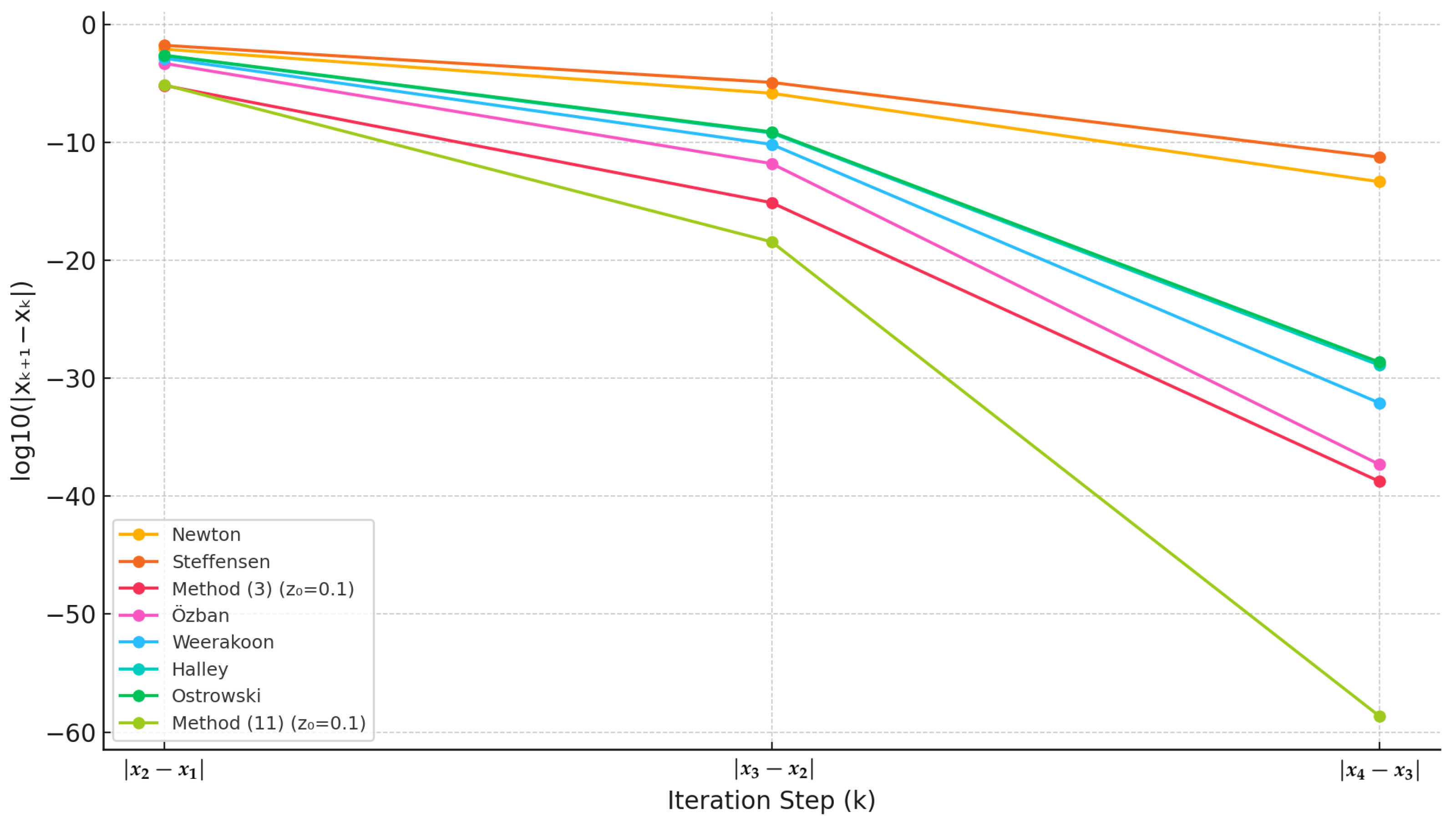
Figure 1 presents a graphical representation of the numerical results shown in Table 1. It is evident from this figure that the proposed method (11) demonstrates superior convergence behavior compared to the existing methods. Specifically, Method (11) reaches the desired root with significantly fewer iterations, indicating higher computational efficiency and faster convergence. This improvement confirms the advantage of the new method in solving nonlinear equations.

It is observed from the numerical results that for each test problem, the approximated computational order of convergence (ACOC) of the proposed method (11) consistently confirms the theoretical convergence order. Furthermore, our method possesses better accuracy than existing methods using only two function evaluations. The proposed method (11) consistently demonstrates faster convergence, higher accuracy, and superior computational order of convergence. This confirms the practical advantage of the proposed method over existing methods.

By comparing efficiency indices of different methods using (2) offers additional insight into the computational efficiency. Efficiency indices of different methods are computed as follows:

$$E\left(3\right)\approx 1.554,E\left(11\right)\approx 1.732,E\left(26\right)=E\left(27\right)\approx 1.414,$$

$$E\left(28\right)=E\left(29\right)=E\left(30\right)=E\left(31\right)\approx 1.442.$$

We observe that the new method (11) is more efficient than the method (3) and the methods of order 2 and 3 as considered above. Moreover, the efficiency index $1.732$ is even higher than the efficiency indices of optimal fourth-order methods (i.e., $E=4^{{\displaystyle \frac{1}{3}}}\approx 1.587$) and of optimal eighth-order methods (i.e., $E=8^{{\displaystyle \frac{1}{4}}}\approx 1.682$) [11,13,31,32,33].

5. Complex Dynamics and Comparison

This section presents the comparison of dynamical analysis of the several iteration schemes in terms of the basins of attraction on a variety of nonlinear problems discussed in Section 4. We acquire a better understanding of the behavior of root-finding techniques by plotting their attractor basins or regions of convergence containing the required root in the complex plane. It is fascinating to see that each iterative scheme produces distinct attractor basins for the same nonlinear problem, which enhances their importance in investigating the root-finding techniques. The border between the attractor basins for consecutive zeros of f indicates a complex fractal structure. Assigning a distinct hue to every basin typically yields beautiful visuals that showcase the effectiveness of iterative techniques. First, in 2001 and 2002, respectively, Stewart [34] and Varona [35] looked into the graphical comparison of a few classical iterative techniques. Plotting the portraits of attractor basins of root-finding algorithms has then become a frequent way for their comparison graphically. Studies on this type of comparison have been conducted more lately; for example, one can see [11,14,16,36]. By plotting the attractor basins, all these papers compared various iterative techniques on simple polynomial functions of the form $z^i-1$, in the complex plane. However, we examine the attractor basins of different methods by visualizing their phase portraits on diverse nonlinear equations presented in Section 4.

To draw attractor basins for a nonlinear function $f\left(z\right)$, a point $z_0$ is chosen as an initial guess from a square $I\subset \mathbb{C}$, containing the required root. Each point in I is then painted with a unique color, specific for each root (except blue), for which an iteration method converges to a simple root of $f\left(z\right)=0$. If, for an initial point, the method fails to converge to any of the roots within 25 iterations and for $|\alpha -z_0|>{10}^{-3}$, then that specific point is marked with color blue (indicating divergence or failure). Brighter shades within each basin represent initial points that converge more quickly, requiring fewer iterations.

A mathematical explanation to obtain basins of attraction for an iteration method is given as follows.

Let $f:\mathbb{C}\to \mathbb{C}$ be a nonlinear function, and let ${\alpha }_1,{\alpha }_2,\dots ,{\alpha }_n\in \mathbb{C}$ denote its simple roots, i.e., $f\left({\alpha }_j\right)=0$ and $f^{\prime }\left({\alpha }_j\right)\ne 0$. Consider an iterative method defined by

$$z_{k+1}=\varphi \left(z_k\right),k=0,1,2,\dots ,$$

to approximate the roots of $f\left(z\right)=0$.

• To visualize the basins of attraction, we proceed as follows:

  1

  Define a square region $I=[a,b]\times [c,d]\subset \mathbb{C}$, which contains the desired roots ${\alpha }_j$.

  2

  For each point $z_0\in I$, use it as an initial guess and apply the iterative method. The iteration continues until one of the following conditions is met:

  • Convergence: The method converges to a root ${\alpha }_j$, i.e., $|z_k-{\alpha }_j|<{10}^{-3}$ for some j, and $k\le 25$.
  • Divergence or failure: The method does not converge to any root within 25 iterations, i.e., for all j, $|z_k-{\alpha }_j|>{10}^{-3}$.

  3

  Coloring scheme:

  • If the iteration converges to a root ${\alpha }_j$, assign a unique color (excluding blue) to the initial point $z_0$ based on ${\alpha }_j$.
  • If the iteration does not converge within 25 iterations, color the point $z_0$ blue, indicating divergence or failure.
  • The brightness of the color is determined by the number of iterations required for convergence: fewer iterations correspond to brighter shades.

The resulting plot is a phase portrait or basins of attraction that visualizes the sets

$$B\left({\alpha }_j\right)=\left\{z_0\in I:\underset{k\to \infty }{lim}{z}_k={\alpha }_j\right\},$$

highlighting the regions in the complex plane from which the iteration converges to each root, as well as the speed of convergence.

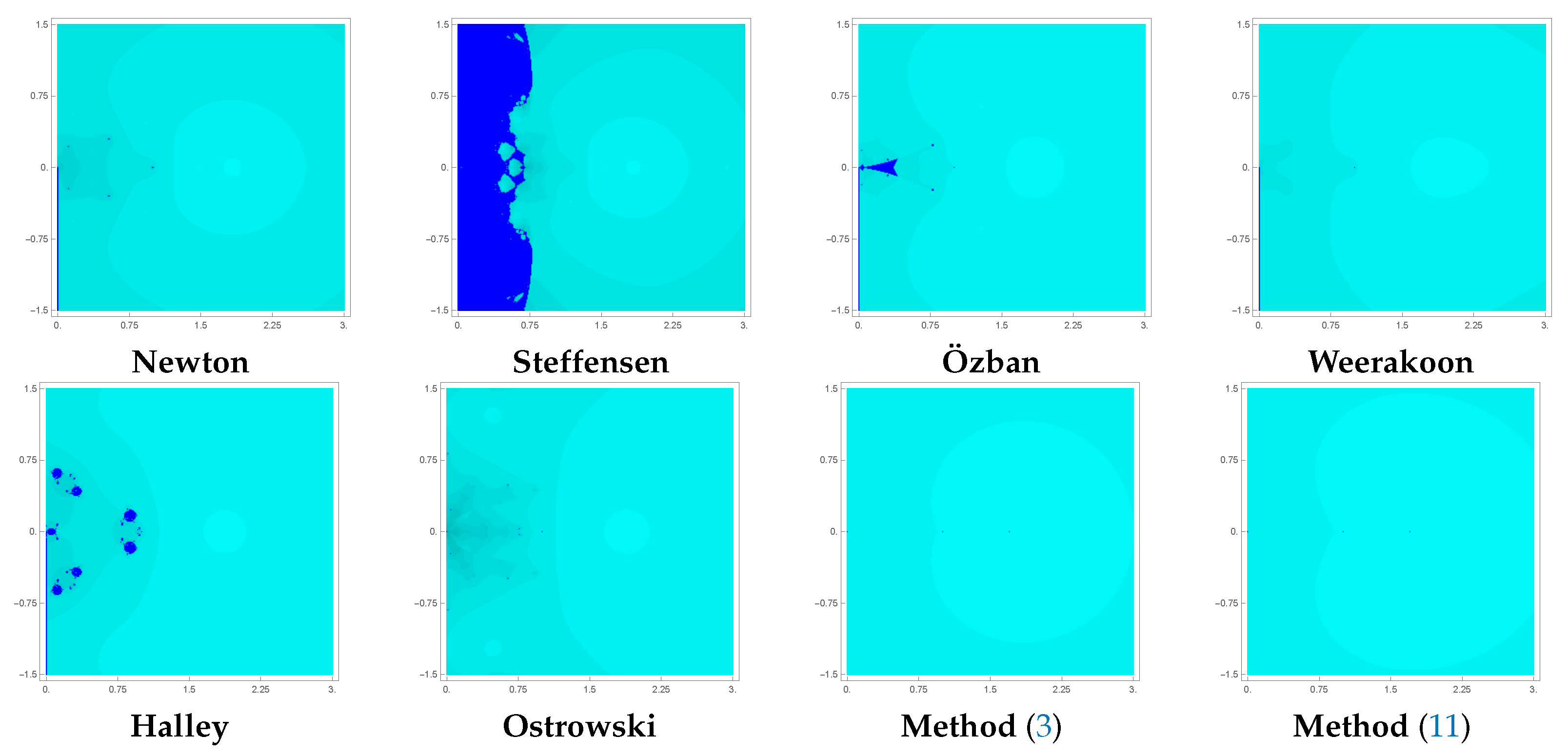
For the attractor basins of $f_1\left(z\right)$ (33), which has a root at $0.13320215082857313\dots$, we chose a grid of $300\times 300$ points in $I=[-5,5]\times [-5,5]\subset \mathbb{C}$. Due to the limited paper space, the significant digits of the root are reduced. The color cyan is assigned to each point in I for which the iteration scheme converges to the root $0.13320215082857313$. The corresponding phase portraits of basins of attraction are displayed in Figure 2. The proposed method (11) and the method (3) have far superior performance regarding the speed and wide areas of convergence in comparison with other classical methods.

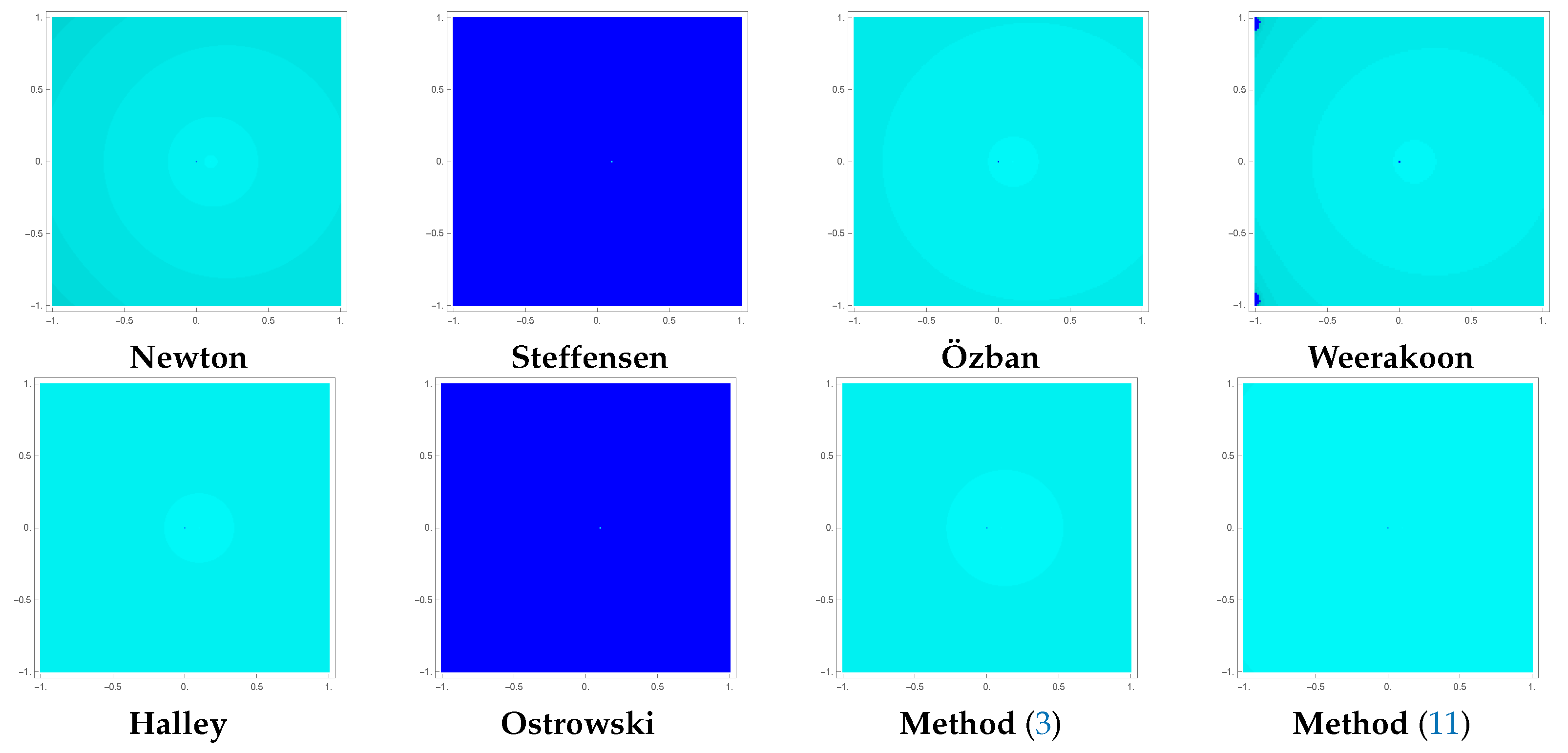
For $f_2\left(z\right)$ (35), which has a zero at $1.84112940685019962\dots$, we chose a grid of $300\times 300$ points in $I=[0,3]\times [-1.5,1.5]\subset \mathbb{C}$. Similar to the previous example, each point of the square I is painted with the color cyan, for which a method converges to the root $1.84112940685019962$. The corresponding portraits of basins are shown in Figure 3, which exhibit the superior performance of the proposed method (11) in terms of convergence speed and convergence region. The proposed method has only two non-convergent points in the selected region.

We have taken a grid of $300\times 300$ points in a square $I=[-5,5]\times [-5,5]\subset \mathbb{C}$ to plot the phase portraits for $f_3\left(z\right)$ (38), which has a zero at $0.10099792968574979$. The color cyan is assigned to each point in I for which an iterative scheme converges to this zero. Figure 4 depicts the corresponding portraits demonstrating the worst behavior (divergence) of the methods by Steffensen (27) and Ostrowski (31) while our method (11) exhibits wider regions of convergence. In particular, the brighter color of basins for the proposed method illustrates its robust convergence in comparison with other methods.

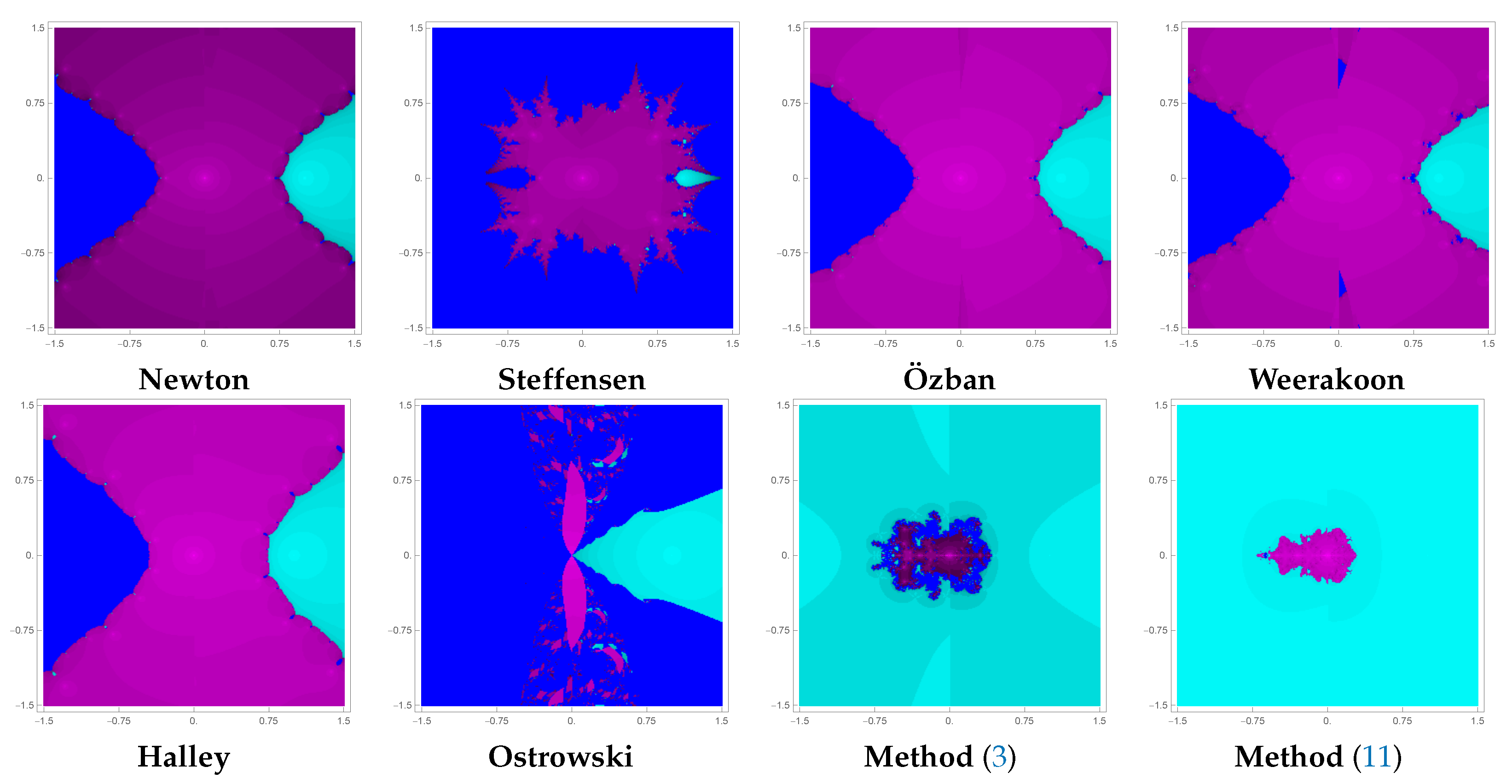
Figure 5 shows the basins of attraction for $f_4\left(z\right)$ (39), for which a grid of $300\times 300$ points is taken in the square $I=[-1.5,1.5]\times [-1.5,1.5]\subset \mathbb{C}$ containing two roots of $f_4\left(z\right)=0$; one multiple root at 0 and a simple root at 1. Each point of the square I is marked with the colors magenta and cyan, for which an iterative scheme converges to the roots 0 and 1, respectively. The blue color indicates that the method fails to converge to any of the zeros. Figure 4 depicts that the methods of Steffensen, Ostrowski, Newton, Ozban, Weerakoon, and Halley possess smaller areas of convergence while the proposed method (11) has wide regions of convergence for the desired root, i.e., $\alpha =1$.

Figure 2, Figure 3, Figure 4 and Figure 5 depict the basins of attraction for the nonlinear problems $f_1-f_4$, providing a visual representation of the convergence behavior of several iterative methods discussed in Section 4. The figures clearly demonstrate that the proposed iterative scheme (11) exhibits significantly wider areas of convergence in comparison to the existing methods in several instances, indicating their robustness and efficiency in solving complex nonlinear problems. This implies that the proposed methods can successfully converge from a broader set of initial guesses, which is a key advantage in practical applications where selecting initial values can be challenging.

Table 5. Comparison of AVGIT, NCP and CPU time for $f_1\left(z\right)$.

Methods	AVGIT	NCP	CPU-Time (s)
Newton	3.348	17150	4.50
Steffensen	1.68	54264	4.46
Özban	2.31	17882	2.29
Weerakoon	2.59	15608	11.5
Halley	2.31	31514	24.97
Ostrowski	3.58	22192	8.84
Method (3)	1.70	34	0.453
Method (11)	1.28	2	0.359

,

Table 6. Comparison of AVGIT, NCP and CPU time for $f_2\left(z\right)$.

Methods	AVGIT	NCP	CPU-Time (s)
Newton	3.13	159	1.18
Steffensen	2.67	19778	11.59
Özban	2.22	456	6.07
Weerakoon	2.28	152	4.31
Halley	2.44	887	3.90
Ostrowski	2.71	10	4.29
Method (3)	1.56	3	1.78
Method (11)	1.37	3	0.26

,

Table 7. Comparison of AVGIT, NCP and CPU time for $f_3\left(z\right)$.

Methods	AVGIT	NCP	CPU-Time (s)
Newton	3.48	1	0.234
Steffensen	Diverges	89999	5.46
Özban	2.27	1	1.57
Weerakoon	2.58	27	3.46
Halley	1.96	1	2.57
Ostrowski	Diverges	89999	5.43
Method (3)	1.88	1	0.218
Method (11)	1.00	1	0.156

and

Table 8. Comparison of AVGIT, NCP and CPU time for $f_4\left(z\right)$.

Methods	AVGIT	NCP	CPU-Time (s)
Newton	13.36	12079	1.64
Steffensen	4.14	63437	7.90
Özban	8.42	12485	5.46
Weerakoon	9.06	11549	8.57
Halley	7.64	14626	4.28
Ostrowski	1.28	71438	5.46
Method (3)	3.92	28	1.89
Method (11)	1.40	20	0.156

provide the comparison of different iteration schemes in terms of average number of iterations (AVGIT), number of non-convergent initial points (NCP) and CPU time (e-time) to plot basins for $f_1\left(z\right),f_2\left(z\right),f_3\left(z\right)$ and $f_4\left(z\right)$, respectively. The proposed method has outperformed other methods in all the metrics, as it has taken less time and performed fewer average iterations to plot the portraits of basins of all functions. Moreover, the basins generated by the proposed method are brighter and wider with fewer diverging points compared with those of the existing iteration methods.

6. Conclusions

In this paper, we have introduced and analyzed a novel higher-order multipoint iteration method for solving nonlinear equations, employing the cubic interpolation to enhance the convergence of the King–Werner method [22]. The proposed approach increases the convergence order from $2.414$ to 3 and improves the efficiency index from $1.554$ to $1.732$, surpassing the efficiency of even optimal fourth and eighth-order methods [11,13,31,32,33]. Through extensive numerical and dynamic experiments, the method’s robustness and superiority have been validated using metrics such as absolute residual error, computational order of convergence, CPU time, and regions of convergence using attractor basins. The method is tested on real-world problems, including Kepler’s equation, isentropic supersonic flow, and the law of population growth, consistently outperforming existing well-known methods. The proposed method is derivative-free and therefore remains applicable even when $f^{\prime }\left(x\right)=0$ at or near the root. This gives it a significant advantage over Newton’s method, particularly for functions that are non-differentiable or have stationary points near the root. The convergence of our method does not depend on the behavior of the derivative but rather on the function evaluations, making it broadly applicable.

Furthermore, the study extended the analysis of convergence and stability beyond traditional polynomial functions like $z^n-1$ to diverse nonlinear functions, providing a more comprehensive understanding of the method’s applicability. The proposed scheme demonstrates faster generation of basins of attraction with wider convergence regions, highlighting its stability and efficiency. These results underscore the method’s potential as a reliable and high-performance tool for solving nonlinear equations in both theoretical and practical applications. The proposed method is designed for solving nonlinear equations where the function is at least continuous and sufficiently differentiable. Its applicability to problems involving non-smooth or discontinuous solutions is limited, as the convergence behavior in such cases may not be guaranteed. This limitation is a subject for future research, particularly extending the method to handle such non-smooth functions.

References

1. Ostrowski, A.M. Solutions of Equations and system of Equations; Academic Press: New York, NY, USA, 1973. [Google Scholar]
2. Traub, J.F. Iterative Methods for the Solution of Equations; Prentice-Hall: Englewood Cliffs, NJ, USA, 1964. [Google Scholar]
3. Petković, M.S.; Neta, B.; Petković, L.D.; Džunić, J. Multipoint methods for solving nonlinear equations: A survey. Appl. Math. Comput. 2014, 226, 635–660. [Google Scholar] [CrossRef]
4. Petković, M.S.; Neta, B.; Petkovixcx, L.D.; Džunić, J. Multipoint Methods for Solving Nonlinear Equations; Elsevier: Amsterdam, The Netherlands, 2013. [Google Scholar]
5. Frontini, M.; Sormani, E. Some variants of Newton’s method with third-order convergence. Appl. Math. Comput. 2003, 140, 419–442. [Google Scholar] [CrossRef]
6. Frontini, M.; Sormani, E. Modified Newton’s method with third-order convergence and multiple roots. J. Comput. Appl. Math. 2003, 156, 345–354. [Google Scholar] [CrossRef]
7. Gander, W. On Halley’s iteration method. Am. Math. Mon. 1985, 92, 131–134. [Google Scholar] [CrossRef]
8. Özban, A.Y. Some new variants of Newton’s method. Appl. Math. Lett. 2004, 17, 677–682. [Google Scholar] [CrossRef]
9. Weerakoon, S.; Fernando, T.G.I. A variant of Newton’s method with accelerated third-order convergence. Appl. Math. Lett. 2000, 13, 87–93. [Google Scholar] [CrossRef]
10. Kung, H.; Traub, J.F. Optimal order of one-point and multipoint iteration. J. ACM 1974, 21, 643–651. [Google Scholar] [CrossRef]
11. Abdullah, S.; Choubey, N.; Dara, S. Optimal fourth-and eighth-order iterative methods for solving nonlinear equations with basins of attraction. J. Appl. Math. Comput. 2024, 70, 3477–3507. [Google Scholar] [CrossRef]
12. Abdullah, S.; Choubey, N.; Dara, S.; Junjua, M.-u.-D.; Abdullah, T. A Robust and Optimal Iterative Algorithm Employing a Weight Function for Solving Nonlinear Equations with Dynamics and Applications. Axioms 2024, 13, 675. [Google Scholar] [CrossRef]
13. Behl, R.; Alshomrani, A.S.; Chun, C. A general class of optimal eighth-order derivative free methods for nonlinear equations. J. Math. Chem. 2020, 58, 854–867. [Google Scholar] [CrossRef]
14. Cordero, A.; Reyes, J.A.; Torregrosa, J.R.; Vassileva, M.P. Stability analysis of a new fourth-order optimal iterative scheme for nonlinear equations. Axioms 2024, 13, 34. [Google Scholar] [CrossRef]
15. Kansal, M.; Sharma, H. Analysis of optimal iterative methods from a dynamical point of view by studying their stability properties. J. Math. Chem. 2024, 62, 198–221. [Google Scholar] [CrossRef]
16. Moscoso-Martinez, M.; Chicharro, F.I.; Cordero, A.; Torregrosa, J.R.; Urena-Callay, G. Achieving Optimal Order in a Novel Family of Numerical Methods: Insights from Convergence and Dynamical Analysis Results. Axioms 2024, 13, 458. [Google Scholar] [CrossRef]
17. Petković, L.D.; Petković, M.S.; Džunić, J. A class of three-point root-solvers of optimal order of convergence. Appl. Math. Comput. 2010, 216, 671–676. [Google Scholar] [CrossRef]
18. Sharma, J.R.; Kumar, S.; Singh, H. A new class of derivative-free root solvers with increasing optimal convergence order and their complex dynamics. SeMA 2023, 80, 333–352. [Google Scholar] [CrossRef]
19. Wang, X.; Liu, L. New eighth-order iterative methods for solving nonlinear equations. Comput. Appl. Math. 2010, 234, 1611–1620. [Google Scholar] [CrossRef]
20. Zheng, Q.; Li, J.; Huang, F. An optimal Steffensen-type family for solving nonlinear equations. Appl. Math. Comput. 2011, 217, 9592–9597. [Google Scholar] [CrossRef]
21. King, R.F. A family of fourth-order methods for nonlinear equations. SIAM J. Numer. Anal. 1973, 10, 876–879. [Google Scholar] [CrossRef]
22. Ren, H.; Argyors, I.K. On the convergence of King-Werner-type methods of order 1 + 2 free of derivative. Appl. Math. Comput. 2015, 256, 148–159. [Google Scholar]
23. Sharma, J.R.; Kumar, S.; Cesarano, C. An Efficient Derivative Free One-Point Method with Memory for Solving Nonlinear Equations. Mathematics 2019, 7, 604. [Google Scholar] [CrossRef]
24. Sharma, J.R.; Argyros, I.K.; Kumar, S. A faster King-Werner-type iteration and its convergence analysis. Appl. Anal. 2019, 99, 2526–2542. [Google Scholar] [CrossRef]
25. Ortega, J.M.; Rheinboldt, W.C. Iterative Solution of Nonlinear Equations in Several Variables; Academic Press: New York, NY, USA, 1970. [Google Scholar]
26. Steffensen, I.F. Remark on iteration. Skand. Aktuarietidskr 1933, 16, 64–72. [Google Scholar] [CrossRef]
27. Cordero, A.; Torregrosa, J.R. Variants of Newton’s method using fifth-order quadrature formulas. Appl. Math. Comput. 2007, 190, 686–698. [Google Scholar] [CrossRef]
28. Danby, J.M.A.; Burkardt, T.M. The solution of Kepler’s equation. I. Celest. Mech. 1983, 40, 95–107. [Google Scholar] [CrossRef]
29. Hoffman, J.D. Numerical Methods for Engineers and Scientists; McGraw-Hill Book Company: New York, NY, USA, 1992. [Google Scholar]
30. Burden, R.L.; Faires, J.D. Numerical Analysi; Brooks/Cole: Boston, MA, USA, 2005. [Google Scholar]
31. Bi, W.; Wu, Q.; Ren, H. A new family of eight-order iterative methods for solving nonlinear equations. Appl. Math. Comput. 2009, 214, 236–245. [Google Scholar]
32. Cordero, A.; Hueso, J.L.; Martínez, E.; Torregrosa, J.R. A new technique to obtain derivative-free optimal iterative methods for solving nonlinear equations. J. Comput. Appl. Math. 2013, 252, 95–102. [Google Scholar] [CrossRef]
33. Geum, Y.H.; Kim, Y.I. A multi-parameter family of three-step eighth-order iterative methods locating a simple root. Appl. Math. Comput. 2010, 215, 3375–3382. [Google Scholar] [CrossRef]
34. Stewart, B.D. Attractor Basins of Various Root-Finding Methods. Ph.D. Thesis, Naval Postgraduate School, Monterey, CA, USA, 2001. [Google Scholar]
35. Varona, J.L. Graphic and numerical comparison between iterative methods. Math. Intell. 2002, 24, 37–47. [Google Scholar] [CrossRef]
36. Varona, J.L. An Optimal Thirty-Second-Order Iterative Method for Solving Nonlinear Equations and a Conjecture. Qual. Theory Dyn. Syst. 2022, 21, 39. [Google Scholar] [CrossRef]
Figure 1. Graphical comparison of the convergence behavior of different iteration methods for f 1 .
Axioms 14 00360 g001
Figure 2. Attractor basins for f 1 ( z ) using different iteration methods.
Axioms 14 00360 g002
Figure 3. Attractor basins for f 2 ( z ) using different iteration methods.
Axioms 14 00360 g003
Figure 4. Attractor basins for f 3 ( z ) using different iteration methods.
Axioms 14 00360 g004
Figure 5. Attractor basins for f 4 ( z ) using different iteration methods.
Axioms 14 00360 g005