An Efficient and Stable Caputo-Type Inverse Fractional Parallel Scheme for Solving Nonlinear Equations

Abstract

Nonlinear problems, which often arise in various scientific and engineering disciplines, typically involve nonlinear equations or functions with multiple solutions. Analytical solutions to these problems are often impossible to obtain, necessitating the use of numerical techniques. This research proposes an efficient and stable Caputo-type inverse numerical fractional scheme for simultaneously approximating all roots of nonlinear equations, with a convergence order of $2\psi +2$. The scheme is applied to various nonlinear problems, utilizing dynamical analysis to determine efficient initial values for a single root-finding Caputo-type fractional scheme, which is further employed in inverse fractional parallel schemes to accelerate convergence rates. Several sets of random initial vectors demonstrate the global convergence behavior of the proposed method. The newly developed scheme outperforms existing methods in terms of accuracy, consistency, validation, computational CPU time, residual error, and stability.

1. Introduction

Solving nonlinear equations is a fundamental problem in science and engineering, with a history dating back to the early days of modern mathematics. These equations, characterized by non-trivial relationships between variables, are crucial for simulating and understanding complex natural phenomena such as biological interactions, turbulent fluid dynamics, and chaotic systems [1,2,3]. The importance of solving nonlinear equations lies in their ability to provide precise descriptions and predictions of these systems, thereby leading to significant advances across various scientific and engineering disciplines [4]. Recent developments in computational methods and the increasing complexity of modern engineering problems have heightened the need for efficient and accurate solutions to nonlinear equations. For instance, in physics, solving Maxwell’s equations for electromagnetism [5] and the Navier–Stokes equations for fluid dynamics [6] is essential for understanding and predicting electromagnetic wave propagation [7] and turbulent flows [8]. These solutions are critical for designing advanced technologies in telecommunications, aerospace, and renewable energy [9,10]. In engineering, nonlinear equations are used to develop control systems that optimize performance and ensure stability in sectors such as aerospace, automotive, and manufacturing. The design of structures to withstand dynamic loads and the creation of sophisticated algorithms for digital signal processing also rely heavily on these equations [11]. In biology and medicine, nonlinear models help replicate the behavior of complex biological systems [12], enhance our understanding of brain networks [13], and improve disease prediction models [14]. Despite their significance, solving nonlinear equations remains a difficult task due to the equations’ inherent complexity and the need for high computational resources. Recent progress in numerical techniques, such as adaptive methods, machine learning algorithms, and parallel computing, offer promising routes for tackling these challenges.

In this paper, we address the solution of fractional differential equations of the form

$$\left\{\begin{array}{c}{}_{\check{c}}ᘐ_{{\psi }_1}^{n\psi }g\left(x\right)+{\vartheta }^{[\ast ]}g\left(x\right)=f(x,g\left(x\right));x\in \left[x_0,x_1\right]\\ g\left(x_0\right)={\theta }_0^{[\ast ]},\\ g^{\prime }\left(x_0\right)={\theta }_1^{[\ast ]},\\ ⋮\\ g^{(n-1)\psi }\left(x_0\right)={\theta }_{n-1}^{[\ast ]},\end{array}\right.$$

(1)

where ${\vartheta }^{[\ast ]}$ is free parameter and ${\theta }_0^{[\ast ]},{\theta }_1^{[\ast ]},\dots ,{\theta }_{n-1}^{[\ast ]}\in \mathbb{R}.$ Differential equations of both integer and fractional orders [15] are crucial for simulating phenomena in physical science and engineering that require precise solutions [16]. Fractional-order differential equations, for example, effectively describe the memory and hereditary characteristics of viscoelastic materials and anomalous diffusion processes [17]. Accurate solutions to these equations are critical for understanding and designing systems with complex behaviors. Solving fractional nonlinear problems

$$g\left(x\right)=0,$$

(2)

requires advanced numerical iterative methods to obtain approximate solutions, see e.g., [18,19,20]. The intrinsic non-locality of these type of models, where the derivative at a point depends on the entire function’s history, makes them notoriously challenging to solve both analytically and numerically. Exact techniques [21], analytical techniques [22,23,24], or direct numerical methods, such as explicit single-step methods [25], multi-step methods [26], and hybrid block methods [27], have significant limitations, including high computational costs, stability issues, and sensitivity to small errors.

Numerical techniques for solving such equations can be classified into two groups: those that find a single solution at a time and those that find all solutions simultaneously. Well-known methods for finding simple roots include the Newton method [28], the Halley method [29], the Chun method [30], the Ostrowski method [31], the King method [32], the Shams method [33], the Cordero method [34], the Mir method [35], the Samima method [36], and the Neta method [37]. For multi-step methods, see, for example, Refs. [38,39] and references therein. Recent studies by Torres-Hernandez et al. [40], Akgül et al. [41], Gajori et al. [42], and Kumar et al. [43] describe fractional versions of single root-finding techniques with various fractional derivatives. These techniques are versatile and often straightforward to implement but have several significant drawbacks. While these methods converge rapidly near initial guesses, they can diverge if the guess is far from the solution or if the function is complex. They are sensitive to initial assumptions, requiring precise estimations for each root, making them time-consuming and computationally intensive. Evaluating both the function and its derivative increases computational costs, especially for complex functions. Additionally, distinguishing between real and complex roots can be challenging without modifications. In contrast, parallel root-finding methods offer greater stability, consistency, and global convergence compared to single root-finding techniques. They can be implemented on parallel computer architectures, utilizing multiple processes to approximate all solutions to (2) simultaneously.

Among parallel numerical schemes, the Weierstrass–Durand–Kerner approach [44] is particularly attractive from a computational standpoint. This method is given by

$$y_i^{\left[l\right]}=x_i^{\left[l\right]}-w\left(x_i^{\left[l\right]}\right),$$

(3)

where

$$w\left(x_i^{\left[l\right]}\right)={\displaystyle \frac{g\left(x_i^{\left[l\right]}\right)}{\underset{\stackrel{j=1}{j\ne i}}{\stackrel{n}{\Pi }}\left(x_i^{\left[l\right]}-x_j^{\left[l\right]}\right)}},(i,j=1,\dots ,n),$$

(4)

is Weierstrass’ correction. Method (3) has local quadratic convergence. Nedzibov et al. [45] present the modified Weierstrass method,

$$y_i^{\left[l\right]}={\displaystyle \frac{{\left(x_i^{\left[l\right]}\right)}^2\underset{\stackrel{j=1}{j\ne i}}{\stackrel{n}{\Pi }}\left(x_i^{\left[l\right]}-x_j^{\left[l\right]}\right)}{x_i^{\left[l\right]}\underset{\stackrel{j=1}{j\ne i}}{\stackrel{n}{\Pi }}\left(x_i^{\left[l\right]}-x_j^{\left[l\right]}\right)+g\left(x_i^{\left[l\right]}\right)}},$$

(5)

also known as the inverse Weierstrass method, which has quadratic convergence. The inverse parallel schemes outperform the classical simultaneous methods because the inverse parallel scheme efficiently handles nonlinear equations by utilizing parallel processing to accelerate convergence. It reduces computing time and improves accuracy by dynamically adapting to the unique properties of the problem. This strategy is especially useful in large-scale or complicated systems where conventional methods may be too slow or ineffectual. Shams et al. [46] presented the following inverse parallel scheme:

$$y_i^{\left[l\right]}=x_i^{\left[l\right]}-{\displaystyle \frac{w\left(x_i^{\left[l\right]}\right)\left(1+g\left(x_i^{\left[l\right]}\right)\right)}{\left(1+\left(1-\alpha g\left(x_i^{\left[l\right]}\right)\right)\right)+\frac{w\left(x_i^{\left[l\right]}\right)}{x_i^{\left[l\right]}}\left(1+g\left(x_i^{\left[l\right]}\right)\right)}}.$$

(6)

Inverse parallel scheme (6) has local quadratic convergence.

In 1977, Ehrlich [47] introduced a convergent simultaneous method of the third order given by

$$y_i^{\left[l\right]}=x_i^{\left[l\right]}-{\displaystyle \frac{1}{\frac{1}{N_i\left(x_i^{\left[l\right]}\right)}-{\displaystyle \sum _{\stackrel{j=1}{j\ne i}}^n}\left(\frac{1}{\left(x_i^{\left[l\right]}-x_j^{\left[l\right]}\right)}\right)}},$$

(7)

where $N_i\left(x_i^{\left[l\right]}\right)={\displaystyle \frac{g\left(x_j^{\left[l\right]}\right)}{g^{\prime }\left(x_j^{\left[l\right]}\right)}}.$ Using $x_j^{\left[l\right]}=u_j^{\left[l\right]}$ as a correction in (4), Petkovic et al. [48] accelerated the convergence order from three to six:

$$y_i^{\left[l\right]}=x_i^{\left[l\right]}-{\displaystyle \frac{1}{\frac{1}{N_i\left(x_i^{\left[l\right]}\right)}-{\displaystyle \sum _{\stackrel{j=1}{j\ne i}}^n}\left(\frac{1}{\left(x_i^{\left[l\right]}-u_j^{\left[l\right]}\right)}\right)}},$$

(8)

where $u_j^{\left[l\right]}=x_j^{\left[l\right]}-{\displaystyle \frac{g\left(s_j^{\left[l\right]}\right)-g\left(x_j^{\left[l\right]}\right)}{2g\left(s_j^{\left[l\right]}\right)-g\left(x_j^{\left[l\right]}\right)}}{\displaystyle \frac{g\left(x_j^{\left[l\right]}\right)}{g^{\prime }\left(x_j^{\left[l\right]}\right)}}$, and $s_j^{\left[l\right]}=x_j^{\left[l\right]}-{\displaystyle \frac{g\left(x_j^{\left[l\right]}\right)}{g^{\prime }\left(x_j^{\left[l\right]}\right)}}$.

Except for the Caputo derivative, all fractional-type derivatives fail to satisfy $\left[{ᘐ}^{\psi }\right]\left(1\right)=0$ if $\psi$ is not a natural number. Therefore, we will cover some basic ideas in fractional calculus, as well as the fractional iterative approach for solving nonlinear equations using Caputo-type derivatives.

Definition 1

(Gamma Function). The Gamma function, also known as the generalized factorial function, is defined as follows [49]:

$$\Gamma \left(x\right)=\underset{0}{\overset{+\infty }{\int }}{u}^{x-1}{e}^{-u}du,$$

(9)

where $x>0$, $\Gamma \left(1\right)=1$, and $\Gamma (n+1)=n!$ for $n\in N.$

Definition 2

(Caputo Fractional Derivative). For

$$g:\mathbb{R}\to \mathbb{R},\left(\begin{array}{c}g\in {\mathbb{C}}^{+\infty }\left(\left[\psi ,x\right]\right),-\infty <\psi <x<+\infty ,\psi \ge 0,\\ m=\left[\psi \right]+1\end{array}\right)$$

(10)

the Caputo fractional derivative [50] of order ψ is defined as

$$\left[{}_{\check{c}}ᘐ_{{\psi }_1}^{\psi }\right]g\left(x\right)=\left\{\begin{array}{c}{\displaystyle \frac{1}{\Gamma (m-\psi )}}\underset{0}{\overset{x}{\int }}\left[{\displaystyle \frac{d^m}{d{t}^m}}g\left(t\right){\displaystyle \frac{1}{{\left(x-t\right)}^{\psi -m+1}}}\right]dt,\psi \in N,\\ {\displaystyle \frac{d^{m-1}}{d{t}^m-1}}g\left(x\right),\psi =m-1\in N\cup \left\{0\right\},\end{array}\right.$$

(11)

where $\Gamma \left(x\right)$ is the Gamma function with $x>0.$

Theorem  1.

Suppose $\left[{}_{\check{c}}ᘐ_{{\psi }_1}^{\gamma \psi }\right]g\left(x\right)\in C\left(\left[{\psi }_1,{\psi }_2\right]\right)$ for $\gamma =1,\dots ,n+1$ where $\psi \in \left(0,1\right]$. Then, the Generalized Taylor Formula [51] is given by

$$g\left(x\right)=\left[{\displaystyle \sum _{i=0}^n}\left[{}_{\check{c}}ᘐ_{{\psi }_1}^{i\psi }\right]g\left({\psi }_1\right){\displaystyle \frac{{\left(x-{\psi }_1\right)}^{i\psi }}{\Gamma (i\psi +1)}}+\left[{}_{\check{c}}ᘐ_{{\psi }_1}^{\left(n+1\right)\psi }\right]g\left(\xi \right){\displaystyle \frac{{\left(x-{\psi }_1\right)}^{\left(n+1\right)\psi }}{\Gamma (\left(n+1\right)\psi +1)}}\right],$$

(12)

where

$${\psi }_1\le \xi \le x,\forall x\in \left({\psi }_1,{\psi }_2\right],$$

and

$$\left[{}_{\check{c}}ᘐ_{{\psi }_1}^{n\psi }\right]=\left[\left[{}_{\check{c}}ᘐ_{{\psi }_1}^{\psi }\right].\left[{}_{\check{c}}ᘐ_{{\psi }_1}^{\psi }\right]\dots \left[{}_{\check{c}}ᘐ_{{\psi }_1}^{\psi }\right](n-times)\right].$$

(13)

Consider the Caputo-type Taylor expansion of $g\left(x\right)$ near ${\psi }_1=\xi$ as

$$g\left(x\right)=\left[{\displaystyle \frac{\left[{}_{\check{c}}ᘐ_{\xi }^{1\psi }\right]g\left(\xi \right)}{\Gamma (+1)}}{\left(x-\xi \right)}^{\psi }+{\displaystyle \frac{\left[{}_{\check{c}}ᘐ_{\xi }^{2\psi }\right]g\left(\xi \right)}{\Gamma (2\psi +1)}}{\left(x-\xi \right)}^{2\psi }+O{\left(x-\xi \right)}^{3\psi }\right].$$

(14)

Taking ${\displaystyle \frac{\left[{}_{\check{c}}ᘐ_{\xi }^{1\psi }\right]g\left(\xi \right)}{\Gamma (\psi +1)}}$ as a common factor, we have

$$g\left(x\right)=\left[{\displaystyle \frac{\left[{}_{\check{c}}ᘐ_{\xi }^{1\psi }\right]g\left(\xi \right)}{\Gamma (\psi +1)}}\left[\begin{array}{c}{\left(x-\xi \right)}^{\psi }+\\ {\check{c}}_2{\left(x-\xi \right)}^{2\psi }\end{array}\right]+O{\left(x-\xi \right)}^{3\psi }\right],$$

(15)

where

$${\check{c}}_j={\displaystyle \frac{\Gamma (\psi +1)}{\Gamma (\gamma \psi +1)}}{\displaystyle \frac{\left[{}_{\check{c}}ᘐ_{\xi }^{\gamma \psi }\right]g\left(\xi \right)}{\left[{}_{\check{c}}ᘐ_{\xi }^{\psi }\right]g\left(\xi \right)}},\gamma =2,3,\dots$$

The corresponding Caputo-type derivative of $g\left(x\right)$ arround $\xi$ is

$$\left[{}_{\check{c}}ᘐ_{\xi }^{\psi }\right]g\left(x\right)=\left[{\displaystyle \frac{\left[{}_{\check{c}}ᘐ_{\xi }^{1\psi }\right]g\left(\xi \right)}{\Gamma (\psi +1)}}\left[\begin{array}{c}\Gamma (\psi +1)+\\ {\displaystyle \frac{\Gamma (2\psi +1)}{\Gamma (\psi +1)}}{\check{c}}_2{\left(x-\xi \right)}^{\psi }\end{array}\right]+O{\left(x-\xi \right)}^{2\psi }\right].$$

(16)

These expansions are used in the convergence analysis of the proposed method.

Using the Caputo-type fractional version of the classical Newton’s method, Candelario et al. [52] presented the following variant:

$$y^{\left[l\right]}=x^{\left[l\right]}-{\left(\Gamma (\psi +1){\displaystyle \frac{g\left(x^{\left[l\right]}\right)}{\left[{}_{\check{c}}ᘐ_{{\psi }_1}^{\psi }\right]g\left(x^{\left[l\right]}\right)}}\right)}^{1/\psi },$$

(17)

where $\left[{}_{\check{c}}ᘐ_{{\psi }_1}^{\psi }\right]g\left(x_i\right)\approx \left[{}_{\check{c}}ᘐ_{\xi }^{\psi }\right]g\left(\xi \right)$ for any $\psi \in \mathbb{R}.$ The error equation satisfied by the fractional Newton method’s order of convergence, which is $\psi +1$, is

$$e^{\left[\ast \right]}=\left[{\displaystyle \frac{\Gamma (\psi +1)-\Gamma (\psi +1)}{\Gamma (\psi +1)}}{\check{c}}_2{\left(e^{\left[l\right]}\right)}^{\psi +1}+O\left({\left(e^{\left[l\right]}\right)}^{2\psi +1}\right)\right],$$

(18)

where $e^{\left[\ast \right]}=y^{\left[l\right]}-\xi$ and $e^{\left[l\right]}=x^{\left[l\right]}-\xi$ and ${\check{c}}_j={\displaystyle \frac{\Gamma (\psi +1)}{\Gamma (\gamma \psi +1)}}{\displaystyle \frac{\left[{}_{\check{c}}ᘐ_{\xi }^{\gamma \psi }\right]g\left(\xi \right)}{\left[{}_{\check{c}}ᘐ_{\xi }^{\psi }\right]g\left(\xi \right)}},\gamma =2,3,\dots$

The rest of the study is organized as follows: following the introduction, Section 2 investigates the construction, convergence, and stability analysis of fractional-order schemes for solving (2). Section 3 presents the development and analysis of a simultaneous method for determining all solutions to nonlinear equations. Section 4 evaluates the efficiency and stability of the proposed approach through numerical results and compares it with existing methods. Finally, Section 5 concludes the paper with a summary of findings and suggestions for future research.

2. Fractional Scheme Construction and Analysis

The fractional-order iterative method is a powerful tool for solving nonlinear equations, offering faster and more accurate convergence compared to classical algorithms. Shams et al. [53] proposed the following single-step fractional iterative method as

$$y^{\left[l\right]}=x^{\left[l\right]}-{\left(\left(\Gamma (\psi +1){\displaystyle \frac{g\left(x^{\left[l\right]}\right)}{\left[{}_{\check{c}}ᘐ_{{\psi }_1}^{\psi }\right]g\left(x^{\left[l\right]}\right)}}\right)\left[{\displaystyle \frac{1}{1-\alpha \frac{g\left(x^{\left[l\right]}\right)}{1+g\left(x^{\left[l\right]}\right)}}}\right]\right)}^{1/\psi },$$

(19)

The order of convergence of the method in (19) is $2\psi +1$, which satisfies the following error equation:

$$e_i^{\left[\ast \right]}={\displaystyle \frac{\left(\left(\alpha +{\check{c}}_2\right){\Gamma }^2(\psi +1)-{\check{c}}_2\Gamma (2\psi +1)\right)}{\psi \Gamma (\psi +1)}}{\check{c}}_2{\left(e^{\left[l\right]}\right)}^{\psi +1}+O\left({\left(e^{\left[l\right]}\right)}^{2\psi +1}\right),$$

(20)

where $e^{\left[\ast \right]}=y^{\left[l\right]}-\xi$, $e^{\left[l\right]}=x^{\left[l\right]}-\xi$ and ${\check{c}}_j={\displaystyle \frac{\Gamma (\psi +1)}{\Gamma (\gamma \psi +1)}}{\displaystyle \frac{\left[{}_{\check{c}}ᘐ_{\xi }^{\gamma \psi }\right]g\left(\xi \right)}{\left[{}_{\check{c}}ᘐ_{\xi }^{\psi }\right]g\left(\xi \right)}},\gamma =2,3,\dots$ The Caputo-type fractional version of (20) was proposed in [54] as

$$v^{\left[l\right]}=y^{\left[l\right]}-{\left(\Gamma (\psi +1){\displaystyle \frac{g\left(y^{\left[l\right]}\right)}{\left[{}_{\check{c}}ᘐ_{{\psi }_1}^{\psi }\right]g\left(x^{\left[l\right]}\right)}}\right)}^{1/\psi },$$

(21)

where $y^{\left[l\right]}=x^{\left[l\right]}-{\left(\Gamma (\psi +1){\displaystyle \frac{g\left(x^{\left[l\right]}\right)}{\left[{}_{\check{c}}ᘐ_{{\psi }_1}^{\psi }\right]g\left(x^{\left[l\right]}\right)}}\right)}^{1/\psi },$ and $\left[{}_{\check{c}}ᘐ_{{\psi }_1}^{\psi }\right]g\left(x^{\left[l\right]}\right)\approx \left[{}_{\check{c}}ᘐ_{\xi }^{\psi }\right]g\left(\xi \right)$ for any $\psi \in \mathbb{R}.$ The order of convergence of the (21) technique is $2\psi +1$, which satisfies the following error equation:

$$e^{\left[\ast \right]}={\displaystyle \frac{\Gamma (\psi +1)-\Gamma (\psi +1)}{\Gamma (\psi +1)}}{\check{c}}_2{\left(e^{\left[l\right]}\right)}^{2\psi +1}+O\left({\left(e^{\left[l\right]}\right)}^{3\psi +1}\right),$$

(22)

where $e^{\left[\ast \right]}=v^{\left[l\right]}-\xi$, $e^{\left[l\right]}=e^{\left[l\right]}-\xi$ and ${\check{c}}_j={\displaystyle \frac{\Gamma (\psi +1)}{\Gamma (\gamma \psi +1)}}{\displaystyle \frac{\left[{}_{\check{c}}ᘐ_{\xi }^{\gamma \psi }\right]g\left(\xi \right)}{\left[{}_{\check{c}}ᘐ_{\xi }^{\psi }\right]g\left(\xi \right)}},\gamma =2,3,\dots$

In this paper, we focus on the technique described in [55], which offers faster convergence speed, higher accuracy, better processing efficiency, and more robustness compared to other single root-finding methods. We extend this method to handle fractional derivatives, enabling the more precise modeling of systems with memory and non-local effects. The original method is given by

$$u^{\left[l\right]}=x^{\left[l\right]}-{\displaystyle \frac{1}{2}}\left(3-{\displaystyle \frac{g^{\prime }\left({\varsigma }^{\left[l\right]}\right)}{g^{\prime }\left(x^{\left[l\right]}\right)}}\right){\displaystyle \frac{g\left(x^{\left[l\right]}\right)}{g^{\prime }\left(x^{\left[l\right]}\right)}},$$

(23)

where ${\varsigma }^{\left[l\right]}=x^{\left[l\right]}-{\displaystyle \frac{g\left(x^{\left[l\right]}\right)}{g^{\prime }\left(x^{\left[l\right]}\right)}}.$ By incorporating the Caputo-type fractional derivative into (23), we propose the following fractional version of the single root finding method:

$$u^{\left[l\right]}=x^{\left[l\right]}-{\left({\displaystyle \frac{1}{2}}\left(3-{\displaystyle \frac{\left[{}_{\check{c}}ᘐ_{{\psi }_1}^{\psi }\right]g\left({\varsigma }^{\left[l\right]}\right)}{\left[{}_{\check{c}}ᘐ_{{\psi }_1}^{\psi }\right]g\left(x^{\left[l\right]}\right)}}\right){\displaystyle \frac{g\left(x^{\left[l\right]}\right)}{\left[{}_{\check{c}}ᘐ_{{\psi }_1}^{\psi }\right]g\left(x^{\left[l\right]}\right)}}\right)}^{1/\psi },$$

(24)

where ${\varsigma }^{\left[l\right]}=x^{\left[l\right]}-{\left(\Gamma (\psi +1){\displaystyle \frac{g\left(x^{\left[l\right]}\right)}{\left[{}_{\check{c}}ᘐ_{{\psi }_1}^{\psi }\right]g\left(x^{\left[l\right]}\right)}}\right)}^{1/\psi }$. We abbreviate this method as ${\mathrm{SCM}}^{\psi }$.

2.1. Convergence Analysis

For the iterative scheme (23), we prove the following theorem to establish its order of convergence.

Theorem  2.

Let

$$g:ᘐ\subseteq \mathbb{R}\to \mathbb{R}$$

(25)

be a continuous function with fractional derivatives of order $l\psi$ for any $l\ge 0$ and $\psi \in \left(0,1\right]$, containing the exact root ξ of $g\left(x\right)$ in the open interval ᘐ. Let us suppose $\left[{}_{\check{c}}ᘐ_{{\psi }_1}^{\psi }\right]g\left(x\right)$ be continuous and not null at ξ. Furthermore, for a sufficiently close starting value $x_0$, the convergence order of the Caputo-type fractional iterative scheme

$$u^{\left[l\right]}=x^{\left[l\right]}-{\left({\displaystyle \frac{1}{2}}\Gamma \left(\psi +1\right)\left(3-{\displaystyle \frac{\left[{}_{\check{c}}ᘐ_{{\psi }_1}^{\psi }\right]g\left({\varsigma }^{\left[l\right]}\right)}{\left[{}_{\check{c}}ᘐ_{{\psi }_1}^{\psi }\right]g\left(x^{\left[l\right]}\right)}}\right){\displaystyle \frac{g\left(x^{\left[l\right]}\right)}{\left[{}_{\check{c}}ᘐ_{{\psi }_1}^{\psi }\right]g\left(x^{\left[l\right]}\right)}}\right)}^{1/\psi },$$

(26)

is at least $2\psi +1$, and the error equation is

$$e^{\left[\ast \right]}=\left({\Theta }_1^{[\ast ]}+{\Theta }_2^{[\ast ]}+{\Theta }_3^{[\ast ]}\right){\left[e^{\left[l\right]}\right]}^{2\psi +1}+O\left({\left[e^{\left[l\right]}\right]}^{3\psi +1}\right).$$

(27)

where ${\Theta }_1^{[\ast ]}={\displaystyle \frac{{\check{c}}_2^2}{{\psi }^2\left({\Gamma }^2\left(\psi \right)\right)}}+{\displaystyle \frac{3}{2}}{\displaystyle \frac{{\check{c}}_3}{\psi \left(\Gamma \left(\psi \right)\right)}}-{\displaystyle \frac{1}{2}}{\displaystyle \frac{{\check{c}}_3}{{\psi }^2\left({\Gamma }^2\left(\psi \right)\right)}}-{\displaystyle \frac{3}{2}}{\displaystyle \frac{{\left(2^{\psi }\right)}^2\left(\Gamma (\psi +\frac{1}{2})\right){\check{c}}_2}{{\psi }^2{\left(\Gamma \left(\psi \right)\right)}^2\sqrt{\pi }}}$,

${\Theta }_2^{[\ast ]}={\displaystyle \frac{3}{2}}{\displaystyle \frac{{\left(2^{\psi }\right)}^4\left({\Gamma }^2(\psi +\frac{1}{2})\right){\check{c}}_2^2}{{\psi }^3{\left(\Gamma \left(\psi \right)\right)}^3\pi }}-{\displaystyle \frac{3}{2}}{\displaystyle \frac{{\left(2^{\psi }\right)}^4\left({\Gamma }^2(\psi +\frac{1}{2})\right){\check{c}}_2^2}{{\psi }^4{\left(\Gamma \left(\psi \right)\right)}^4\pi }}$, ${\Theta }_3^{[\ast ]}=-{\displaystyle \frac{3}{4}}{\displaystyle \frac{{\check{c}}_2{\check{c}}_3\left({\left(3^{\psi }\right)}^3\Gamma (\psi +\frac{1}{3})\Gamma (\psi +\frac{2}{3})\right)}{{\psi }^2\left({\Gamma }^2\left(\psi \right)\right)\sqrt{\pi }{\left(2^{\psi }\right)}^2\Gamma (\psi +\frac{1}{2})}}+{\displaystyle \frac{1}{2}}{\displaystyle \frac{{\check{c}}_2{\check{c}}_3\left({\left(3^{\psi }\right)}^3\Gamma (\psi +\frac{1}{3})\Gamma (\psi +\frac{2}{3})\right)}{{\psi }^3\left({\Gamma }^3\left(\psi \right)\right)\sqrt{\pi }{\left(2^{\psi }\right)}^2\Gamma (\psi +\frac{1}{2})}},$

${\check{c}}_j={\displaystyle \frac{\Gamma (\psi +1)}{\Gamma (\gamma \psi +1)}}{\displaystyle \frac{\left[{}_{\check{c}}ᘐ_{\xi }^{\gamma \psi }\right]g\left(\xi \right)}{\left[{}_{\check{c}}ᘐ_{\xi }^{\psi }\right]g\left(\xi \right)}},\gamma =2,3,\dots$ and ${\left[\Gamma \left(.\right)\right]}^n={\Gamma }^n(.).$

Proof. 

Let $\xi$ be a root of g and $x^{\left[l\right]}=\xi +e^{\left[l\right]}$. By the Taylor series expansion of $g\left(x^{\left[l\right]}\right)$ and $\left[{}_{\check{c}}ᘐ_{{\psi }_1}^{\psi }\right]g\left(x^{\left[l\right]}\right)$ around $x=\xi ,$ taking $g\left(\xi \right)=0,$ we get

$$g\left(x^{\left[l\right]}\right)={\displaystyle \frac{\left[{}_{\check{c}}ᘐ_{\xi }^{1\psi }\right]g\left(\xi \right)}{\Gamma (\psi +1)}}\left[{\left[e^{\left[l\right]}\right]}^{\psi }+{\check{c}}_2{\left[e^{\left[l\right]}\right]}^{2\psi }+{\check{c}}_3{\left[e^{\left[l\right]}\right]}^{3\psi }\right]+O\left({\left[e^{\left[l\right]}\right]}^{4\psi }\right),$$

(28)

and

$$\left[{}_{\check{c}}ᘐ_{{\psi }_1}^{\psi }\right]g\left(x^{\left[l\right]}\right)={\displaystyle \frac{\left[{}_{\check{c}}ᘐ_{\xi }^{1\psi }\right]g\left(\xi \right)}{\Gamma (\psi +1)}}\left[\begin{array}{c}\Gamma (\psi +1)+{\displaystyle \frac{\Gamma (2\psi +1)}{\Gamma (\psi +1)}}{\check{c}}_2{\left[e^{\left[l\right]}\right]}^{\psi }\\ +{\displaystyle \frac{\Gamma (3\psi +1)}{\Gamma (2\psi +1)}}{\check{c}}_3{\left[e^{\left[l\right]}\right]}^{2\psi }\end{array}\right]+O\left({\left[e^{\left[l\right]}\right]}^{3\psi }\right),$$

(29)

$${\left(\left[{}_{\check{c}}ᘐ_{{\psi }_1}^{\psi }\right]g\left(x^{\left[l\right]}\right)\right)}^{-1}=\left[\begin{array}{c}{\displaystyle \frac{1}{\Gamma (\psi +1)}}-{\Delta }^{\left\{1\right\}}{\left[e^{\left[l\right]}\right]}^{\psi }+{\Delta }^{\left\{2\right\}}{\left[e^{\left[l\right]}\right]}^{2\psi }+\\ {\Delta }^{\left\{3\right\}}{\left[e^{\left[l\right]}\right]}^{3\psi }\end{array}\right]+O\left({\left[e^{\left[l\right]}\right]}^{4\psi }\right),$$

(30)

where ${\Delta }^{\left\{1\right\}}={\displaystyle \frac{\Gamma (2\psi +1)}{\Gamma (\psi +1)}}{\check{c}}_2$, ${\Delta }^{\left\{2\right\}}={\displaystyle \frac{\left(-\frac{\Gamma (3\psi +1)}{\Gamma (\psi +1)\Gamma (2\psi +1)}+\frac{{\left(\Gamma (2\psi +1)\right)}^2}{{\left(\Gamma (\psi +1)\right)}^4}\right)}{\Gamma (\psi +1)}}{\check{c}}_3$, ${\Delta }^{\left\{3\right\}}=\left({\displaystyle \frac{\frac{\Gamma (3\psi +1)}{\Gamma (\psi +1)}{\check{c}}_2{\check{c}}_3-\frac{{\left(\Gamma (2\psi +1)\right)}^3{\check{c}}_2^2-\Gamma (3\psi +1){\left(\Gamma (\psi +1)\right)}^3{\check{c}}_2{\check{c}}_3}{{\left(\Gamma (\psi +1)\right)}^6}}{\Gamma (\psi +1)}}\right).$

Dividing (28) by (29), we have:

$${\displaystyle \frac{g\left(x^{\left[l\right]}\right)}{\left[{}_{\check{c}}ᘐ_{{\psi }_1}^{\psi }\right]g\left(x^{\left[l\right]}\right)}}={\displaystyle \frac{1}{\psi \Gamma \left(\psi \right)}}{\left[e^{\left[l\right]}\right]}^{\psi }+{\Delta }^{\left\{4\right\}}{\left[e^{\left[l\right]}\right]}^{2\psi }+{\Delta }^{\left\{5\right\}}{\left[e^{\left[l\right]}\right]}^{3\psi }+O\left({\left[e^{\left[l\right]}\right]}^{4\psi }\right),$$

(31)

where

$${\Delta }^{\left\{4\right\}}=\left({\displaystyle \frac{{\left(2^{\psi }\right)}^2\Gamma (\psi +\frac{1}{2}){\check{c}}_2}{{\psi }^2{\left(\Gamma \left(\psi \right)\right)}^2\sqrt{\pi }}}+{\displaystyle \frac{{\check{c}}_2}{\psi \Gamma \left(\psi \right)}}\right),$$

$${\Delta }^{\left\{5\right\}}=\left(\begin{array}{c}{\displaystyle \frac{{\left(2^{\psi }\right)}^4{\left(\Gamma (\psi +\frac{1}{2})\right)}^2{\check{c}}_2^2}{{\psi }^3{\left(\Gamma \left(\psi \right)\right)}^3\pi }}-{\displaystyle \frac{{\left(2^{\psi }\right)}^2\Gamma (\psi +\frac{1}{2}){\check{c}}_2^3}{{\psi }^2{\left(\Gamma \left(\psi \right)\right)}^2\sqrt{\pi }}}-\\ {\displaystyle \frac{1}{2}}{\displaystyle \frac{{\check{c}}_3\left(3^{\psi }\sqrt{3}\Gamma (\psi +\frac{1}{3})\Gamma (\psi +\frac{2}{3})\right)}{{\psi }^2{\left(\Gamma \left(\psi \right)\right)}^2\sqrt{\pi }{\left(2^{\psi }\right)}^2\Gamma (\psi +\frac{1}{2})}}+{\displaystyle \frac{{\check{c}}_3}{\psi \Gamma \left(\psi \right)}}\end{array}\right),$$

and

$$\Gamma \left({\displaystyle \frac{1}{\psi }}+1\right)={\displaystyle \frac{1}{\psi }}\Gamma \left({\displaystyle \frac{1}{\psi }}\right).$$

Next,

$${\varsigma }^{\left[l\right]}-\xi =x^{\left[l\right]}-\xi -{\left(\Gamma (\psi +1){\displaystyle \frac{g\left(x^{\left[l\right]}\right)}{\left[{}_{\check{c}}ᘐ_{{\psi }_1}^{\psi }\right]g\left(x^{\left[l\right]}\right)}}\right)}^{1/\psi },$$

and

$${\varsigma }^{\left[l\right]}-\xi ={\Delta }^{\left\{6\right\}}{\left[e^{\left[l\right]}\right]}^{\psi +1}+\left[{\Delta }^{\left\{7\right\}}+{\Delta }^{\left\{8\right\}}\right]{\left[e^{\left[l\right]}\right]}^{2\psi +1}+O\left({\left[e^{\left[l\right]}\right]}^{3\psi +1}\right),$$

where

$${\Delta }^{\left\{6\right\}}=\left(-{\check{c}}_2+{\displaystyle \frac{{\left(2^{\psi }\right)}^2\Gamma (\psi +\frac{1}{2}){\check{c}}_2}{\psi \left(\Gamma \left(\psi \right)\right)\sqrt{\pi }}}\right),$$

$${\Delta }^{\left\{7\right\}}=-{\check{c}}_3+{\displaystyle \frac{{\left(2^{\psi }\right)}^2{\left(\Gamma (\psi +\frac{1}{2})\right)}^2{\check{c}}_2^2}{\psi \left(\Gamma \left(\psi \right)\right)\sqrt{\pi }}}+{\displaystyle \frac{1}{2}}{\displaystyle \frac{{\left(2^{\psi }\right)}^2\Gamma (\psi +\frac{1}{2}){\check{c}}_2^3}{\psi \left(\Gamma \left(\psi \right)\right)\sqrt{\pi }}},$$

$${\Delta }^{\left\{8\right\}}={\displaystyle \frac{1}{2}}{\displaystyle \frac{{\check{c}}_3\left({\left(3^{\psi }\right)}^3\Gamma (\psi +\frac{1}{3})\Gamma (\psi +\frac{2}{3})\right)}{\psi \left(\Gamma \left(\psi \right)\right)\sqrt{\pi }{\left(2^{\psi }\right)}^2\Gamma (\psi +\frac{1}{2})}}-{\displaystyle \frac{{\left(2^{\psi }\right)}^4{\left(\Gamma (\psi +\frac{1}{2})\right)}^2{\check{c}}_2^2}{{\psi }^2{\left(\Gamma \left(\psi \right)\right)}^2\pi }}.$$

Using the generalized binomial theorem ${\left(x+y\right)}^t={\displaystyle \sum _{i=0}^{+\infty }}\left({\displaystyle \genfrac{}{}{0pt}{}{t}{i}}\right)x^{t-i}{y}^i$ where $\left({\displaystyle \genfrac{}{}{0pt}{}{t}{i}}\right)={\displaystyle \frac{\Gamma (t+1)}{i!\Gamma (t-i+1)}},$ expanding $g\left(x_i^{\left[1\right]}\right)$ around $\xi ,$ we have

$$\left[{}_{\check{c}}ᘐ_{{\psi }_1}^{\psi }\right]g\left({\varsigma }^{\left[l\right]}\right)=1+2{\check{c}}_2\left({\Delta }^{\left\{6\right\}}\right){\left[e^{\left[l\right]}\right]}^{\psi +1}+2{\Delta }^{\left\{9\right\}}{\left[e^{\left[l\right]}\right]}^{3\psi +1}+\dots$$

where

$${\Delta }^{\left\{9\right\}}=-{\check{c}}_3+{\displaystyle \frac{{\left(2^{\psi }\right)}^2\left(\Gamma (\psi +\frac{1}{2})\right){\check{c}}_2}{\psi \left(\Gamma \left(\psi \right)\right)\sqrt{\pi }}}+{\displaystyle \frac{1}{2}}{\displaystyle \frac{{\check{c}}_3\left({\left(3^{\psi }\right)}^3\Gamma (\psi +\frac{1}{3})\Gamma (\psi +\frac{2}{3})\right)}{\psi \left(\Gamma \left(\psi \right)\right)\sqrt{\pi }{\left(2^{\psi }\right)}^2\Gamma (\psi +\frac{1}{2})}}-{\displaystyle \frac{{\left(2^{\psi }\right)}^4{\left(\Gamma (\psi +\frac{1}{2})\right)}^2{\check{c}}_2^2}{{\psi }^2{\left(\Gamma \left(\psi \right)\right)}^3\sqrt{\pi }}}.$$

Then,

$${\displaystyle \frac{\left[{}_{\check{c}}ᘐ_{{\psi }_1}^{\psi }\right]g\left({\varsigma }^{\left[l\right]}\right)}{\left[{}_{\check{c}}ᘐ_{{\psi }_1}^{\psi }\right]g\left(x^{\left[l\right]}\right)}}={\displaystyle \frac{1}{\psi \Gamma \left(\psi \right)}}-{\Delta }^{\left\{10\right\}}{e}^{\left[l\right]}+{\Delta }^{\left\{11\right\}}{\left[e^{\left[l\right]}\right]}^{\psi +1}+\dots$$

where

$${\Delta }^{\left\{10\right\}}=\left({\displaystyle \frac{{\left(2^{\psi }\right)}^2\left(\Gamma (\psi +\frac{1}{2})\right){\check{c}}_2}{{\psi }^2{\left(\Gamma \left(\psi \right)\right)}^2\sqrt{\pi }}}\right),{\Delta }^{\left\{11\right\}}=\left(\begin{array}{c}-{\displaystyle \frac{1}{2}}{\displaystyle \frac{{\check{c}}_3\left({\left(3^{\psi }\right)}^3\Gamma (\psi +\frac{1}{3})\Gamma (\psi +\frac{2}{3})\right)}{\psi \left(\Gamma \left(\psi \right)\right)\sqrt{\pi }{\left(2^{\psi }\right)}^2\Gamma (\psi +\frac{1}{2})}}-{\displaystyle \frac{2{\check{c}}_2^2}{\psi \left(\Gamma \left(\psi \right)\right)}}+\\ {\displaystyle \frac{{\left(2^{\psi }\right)}^4\left({\Gamma }^2(\psi +\frac{1}{2})\right){\check{c}}_2^2}{{\psi }^3{\left(\Gamma \left(\psi \right)\right)}^3\pi }}+{\displaystyle \frac{2{\left(2^{\psi }\right)}^2\left(\Gamma (\psi +\frac{1}{2})\right){\check{c}}_2^2}{{\psi }^2{\left(\Gamma \left(\psi \right)\right)}^2\sqrt{\pi }}}\end{array}\right).$$

Therefore, using ${\displaystyle \frac{\left[{}_{\check{c}}ᘐ_{{\psi }_1}^{\psi }\right]g\left({\varsigma }^{\left[l\right]}\right)}{\left[{}_{\check{c}}ᘐ_{{\psi }_1}^{\psi }\right]g\left(x^{\left[l\right]}\right)}}$ in second step, we have

$${\displaystyle \frac{1}{2}}\left(3-{\displaystyle \frac{\left[{}_{\check{c}}ᘐ_{{\psi }_1}^{\psi }\right]g\left({\varsigma }^{\left[l\right]}\right)}{\left[{}_{\check{c}}ᘐ_{{\psi }_1}^{\psi }\right]g\left(x^{\left[l\right]}\right)}}\right)=-{\displaystyle \frac{1}{2\psi \left(\Gamma \left(\psi \right)\right)}}+{\displaystyle \frac{3}{2}}+{\Delta }^{\left\{12\right\}}{e}^{\left[l\right]}+{\Delta }^{\left\{13\right\}}{\left[e^{\left[l\right]}\right]}^{\psi +1}+\dots$$

where

$${\Delta }^{\left\{12\right\}}={\displaystyle \frac{1}{2}}{\displaystyle \frac{{\left(2^{\psi }\right)}^2\left(\Gamma (\psi +\frac{1}{2})\right){\check{c}}_2}{{\psi }^2{\left(\Gamma \left(\psi \right)\right)}^2\sqrt{\pi }}},{\Delta }^{\left\{13\right\}}=\left(\begin{array}{c}{\displaystyle \frac{1}{4}}{\displaystyle \frac{{\check{c}}_3\left({\left(3^{\psi }\right)}^3\Gamma (\psi +\frac{1}{3})\Gamma (\psi +\frac{2}{3})\right)}{\psi \left(\Gamma \left(\psi \right)\right)\sqrt{\pi }{\left(2^{\psi }\right)}^2\Gamma (\psi +\frac{1}{2})}}-{\displaystyle \frac{{\check{c}}_2^2}{\psi \left(\Gamma \left(\psi \right)\right)}}+\\ {\displaystyle \frac{1}{2}}{\displaystyle \frac{{\left(2^{\psi }\right)}^4\left({\Gamma }^2(\psi +\frac{1}{2})\right){\check{c}}_2^2}{{\psi }^3{\left(\Gamma \left(\psi \right)\right)}^3\pi }}+{\displaystyle \frac{2{\left(2^{\psi }\right)}^2\left(\Gamma (\psi +\frac{1}{2})\right){\check{c}}_2^2}{{\psi }^2{\left(\Gamma \left(\psi \right)\right)}^2\sqrt{\pi }}}\end{array}\right).$$

Thus

$$u^{\left[l\right]}-\zeta =x^{\left[l\right]}-\zeta -{\left({\displaystyle \frac{1}{2}}\Gamma \left(\psi +1\right)\left(3-{\displaystyle \frac{\left[{}_{\check{c}}ᘐ_{{\psi }_1}^{\psi }\right]g\left({\varsigma }^{\left[l\right]}\right)}{\left[{}_{\check{c}}ᘐ_{{\psi }_1}^{\psi }\right]g\left(x^{\left[l\right]}\right)}}\right){\displaystyle \frac{g\left(x^{\left[l\right]}\right)}{\left[{}_{\check{c}}ᘐ_{{\psi }_1}^{\psi }\right]g\left(x^{\left[l\right]}\right)}}\right)}^{1/\psi },$$

$$e^{\left[\ast \right]}=e-e+\left({\Theta }_1^{[\ast ]}+{\Theta }_2^{[\ast ]}+{\Theta }_3^{[\ast ]}\right){\left[e^{\left[l\right]}\right]}^{2\psi +1}+\left({\Theta }_4^{[\ast ]}+{\Theta }_5^{[\ast ]}+{\Theta }_6^{[\ast ]}\right){\left[e^{\left[l\right]}\right]}^{3\psi +1}+\dots$$

where

$${\Theta }_1^{[\ast ]}={\displaystyle \frac{{\check{c}}_2^2}{{\psi }^2\left({\Gamma }^2\left(\psi \right)\right)}}+{\displaystyle \frac{3}{2}}{\displaystyle \frac{{\check{c}}_3}{\psi \left(\Gamma \left(\psi \right)\right)}}-{\displaystyle \frac{1}{2}}{\displaystyle \frac{{\check{c}}_3}{{\psi }^2\left({\Gamma }^2\left(\psi \right)\right)}}-{\displaystyle \frac{3}{2}}{\displaystyle \frac{{\left(2^{\psi }\right)}^2\left(\Gamma (\psi +\frac{1}{2})\right){\check{c}}_2}{{\psi }^2{\left(\Gamma \left(\psi \right)\right)}^2\sqrt{\pi }}},$$

$${\Theta }_2^{[\ast ]}={\displaystyle \frac{3}{2}}{\displaystyle \frac{{\left(2^{\psi }\right)}^4\left({\Gamma }^2(\psi +\frac{1}{2})\right){\check{c}}_2^2}{{\psi }^3{\left(\Gamma \left(\psi \right)\right)}^3\pi }}-{\displaystyle \frac{3}{2}}{\displaystyle \frac{{\left(2^{\psi }\right)}^4\left({\Gamma }^2(\psi +\frac{1}{2})\right){\check{c}}_2^2}{{\psi }^4{\left(\Gamma \left(\psi \right)\right)}^4\pi }},$$

$${\Theta }_3^{[\ast ]}=-{\displaystyle \frac{3}{4}}{\displaystyle \frac{{\check{c}}_2{\check{c}}_3\left({\left(3^{\psi }\right)}^3\Gamma (\psi +\frac{1}{3})\Gamma (\psi +\frac{2}{3})\right)}{{\psi }^2\left({\Gamma }^2\left(\psi \right)\right)\sqrt{\pi }{\left(2^{\psi }\right)}^2\Gamma (\psi +\frac{1}{2})}}+{\displaystyle \frac{1}{2}}{\displaystyle \frac{{\check{c}}_2{\check{c}}_3\left({\left(3^{\psi }\right)}^3\Gamma (\psi +\frac{1}{3})\Gamma (\psi +\frac{2}{3})\right)}{{\psi }^3\left({\Gamma }^3\left(\psi \right)\right)\sqrt{\pi }{\left(2^{\psi }\right)}^2\Gamma (\psi +\frac{1}{2})}},$$

$${\Theta }_4^{[\ast ]}=-{\displaystyle \frac{{\check{c}}_2{\check{c}}_3\left({\left(3^{\psi }\right)}^3\Gamma (\psi +\frac{1}{3})\Gamma (\psi +\frac{2}{3})\right)}{{\psi }^4{\left(\Gamma \left(\psi \right)\right)}^4\pi }}-{\displaystyle \frac{1}{4}}{\displaystyle \frac{{\check{c}}_2{\check{c}}_3\left({\left(3^{\psi }\right)}^3\Gamma (\psi +\frac{1}{3})\Gamma (\psi +\frac{2}{3})\right)}{{\psi }^3\left({\Gamma }^3\left(\psi \right)\right)\sqrt{\pi }{\left(2^{\psi }\right)}^2\Gamma (\psi +\frac{1}{2})}},$$

$${\Theta }_5^{[\ast ]}={\displaystyle \frac{{\check{c}}_2{\check{c}}_3}{{\psi }^2\left({\Gamma }^2\left(\psi \right)\right)}}+{\displaystyle \frac{1}{2}}{\displaystyle \frac{{\left(2^{\psi }\right)}^2\left(\Gamma (\psi +\frac{1}{2})\right){\check{c}}_2{\check{c}}_3}{{\psi }^3{\left(\Gamma \left(\psi \right)\right)}^3\sqrt{\pi }}}+{\displaystyle \frac{{\check{c}}_2^3}{{\psi }^2\left({\Gamma }^2\left(\psi \right)\right)\pi }},$$

$${\Theta }_6^{[\ast ]}={\displaystyle \frac{3}{2}}{\displaystyle \frac{{\check{c}}_2^3{\left(2^{\psi }\right)}^6\left({\Gamma }^3(\psi +\frac{1}{2})\right)}{{\psi }^5{\left(\Gamma \left(\psi \right)\right)}^5{\pi }^{\frac{3}{2}}}}-{\displaystyle \frac{4{\check{c}}_2^3{\left(2^{\psi }\right)}^2\left(\Gamma (\psi +\frac{1}{2})\right)}{{\psi }^3\left({\Gamma }^3\left(\psi \right)\right)\sqrt{\pi }}}+{\displaystyle \frac{2{\check{c}}_2^3{\left(2^{\psi }\right)}^4\left({\Gamma }^2(\psi +\frac{1}{2})\right)}{{\psi }^4\left({\Gamma }^4\left(\psi \right)\right)\pi }}.$$

Thus

$$e^{\left[\ast \right]}=\left({\Theta }_1^{[\ast ]}+{\Theta }_2^{[\ast ]}+{\Theta }_3^{[\ast ]}\right){\left[e^{\left[l\right]}\right]}^{2\psi +1}+O\left({\left[e^{\left[l\right]}\right]}^{3\psi +1}\right).$$

Hence, the theorem is proven.    □

2.2. Stability Analysis of the ${\mathit{SCM}}^{\psi }$-Scheme

The stability of single root-finding methods for nonlinear equations is crucial for ensuring the reliability and robustness of the iterative solution process [56]. Stability, in this context, refers to a method’s ability to converge to a real root from an initial guess, even when minor perturbations or errors occur in the calculations. Single root-finding approaches exhibit local convergence around the root, making them effective when the initial guess is sufficiently close to the exact root. However, their stability is influenced by the nature of the function and the initial estimate. If the function is poorly behaved or the initial estimate is far from the root, single root-finding methods may diverge or converge to extraneous fixed points unrelated to the actual roots of the nonlinear equations [57]. The stability of single root-finding methods can be evaluated using concepts from complex dynamical systems, which measure the sensitivity of the root to changes in the input, and convergence criteria, which assess how rapidly the method approaches the root. To minimize the impact of computational errors and ensure consistent and reliable root-finding performance, stability is often achieved by balancing the method’s inherent convergence properties with the careful selection of the initial guess, function parameters, and stopping criteria [58,59]. The following rational map $R\left(x\right)=\left(x-a\right)\left(x-b\right)$ is obtained as

$$R\left(x\right)=x-{\displaystyle \frac{\left[{\left({\vartheta }_1^{[^]}{\vartheta }_{11}^{[^]}\right)}^{1-\psi }+2{\left({\vartheta }_{11}^{[^]}\right)}^{2-\psi }{\vartheta }_4^{[^]}+ab{\vartheta }_5^{[^]}{\left({\vartheta }_{11}^{[^]}\right)}^{\frac{1}{\psi }}\right]{\vartheta }_6^{[^]}}{{\vartheta }_7^{[^]}+\Gamma (2-\psi ){\vartheta }_8^{[^]}}},$$

(32)

where

${\vartheta }_1^{[^]}=\Gamma \left(3-\psi \right)\Gamma \left(1-\psi \right)\left(a+b\right),$

${\vartheta }_2^{[^]}=\left(x-a\right)\left(x-b\right)\Gamma \left(\psi +1\right),$

${\vartheta }_3^{[^]}={\displaystyle \frac{2x^{2-\psi }}{\Gamma \left(3-\psi \right)}}-{\displaystyle \frac{\left(a+b\right)x^{1-\psi }}{\Gamma \left(2-\psi \right)}}+{\displaystyle \frac{ab{x}^{-\psi }}{\Gamma \left(1-\psi \right)}},$

${\vartheta }_4^{[^]}=\Gamma \left(2-\psi \right)\Gamma \left(1-\psi \right),$

${\vartheta }_5^{[^]}=\left[\Gamma \left(3-\psi \right)\Gamma \left(2-\psi \right)+3{\vartheta }_1^{[^]}{x}^{1-\psi }-3\Gamma \left(2-\psi \right)+{\vartheta }_8^{[^]}\right],$

${\vartheta }_6^{[^]}=\Gamma \left(3-\psi \right)\Gamma \left(2-\psi \right)\Gamma \left(1-\psi \right)\Gamma \left(1+\psi \right)\left(x-a\right)\left(x-b\right),$

${\vartheta }_7^{[^]}=-\left(a+b\right)x^{1-\psi }\Gamma \left(3-\psi \right)\Gamma \left(1-\psi \right),$

${\vartheta }_8^{[^]}=a\Gamma \left(3-\psi \right)b{x}^{-\psi -\psi }+2\Gamma \left(1-\psi \right)x^{2-\psi },$

${\vartheta }_{11}^{[^]}=x-{\left({\displaystyle \frac{{\vartheta }_2^{[^]}}{{\vartheta }_3^{[^]}}}\right)}^{{\displaystyle \frac{1}{\psi }}}.$ For $\psi \approx 1$, we have

$$R\left(x\right)=x-{\displaystyle \frac{\left(x-a\right)\left(x-b\right)\left(5x^2-5\left(a+b\right)x+a^2+3ab+b^2\right)}{{\left(-2x+a+b\right)}^3}},$$

(33)

where $a,b\in \mathbb{C}.$ Thus, $R\left(x\right)$ depends on $a,b$, and the variable. Using Möbius transformation $M\left(x\right)={\displaystyle \frac{x-a}{x-b}},$ we see $R\left(x\right)$ is conjugate with operator

$$\mathrm{O}\left(x\right)=MoRo{M}^{-1}\left(x\right)={\displaystyle \frac{x^3\left(x+2\right)}{2x+1}},$$

(34)

for $\psi \approx 1$ and independent of a and b. Therefore, $R\left(x\right)$ exactly fits with:

$$R^{[\ast ]}\left(x\right)={\displaystyle \frac{{\displaystyle \sum _{i=0}^n}\left(a_i{x}^i\right)}{{\displaystyle \sum _{i=0}^n}\left(a_{n-i}{x}^i\right)}};{\left\{a_i\right\}}_{i=0}^n\in R$$

(35)

which has interesting properties [60].

The next proposition examines the fixed points of the rational map, which are essential for understanding the behavior and convergence properties of these schemes.

Proposition  1.

The fixed points of $\mathrm{O}\left(\epsilon \right)$ are as follows:

• ${\epsilon }_0=0$ and ${\epsilon }_{\infty }=\infty$ are super attracting points.
• ${\epsilon }_1=1$ is a repelling point.
• The critical points are 0 and 1, which are super attracting and repelling points, respectively, for $\psi \approx 1.$

Proof. 

The fixed points of $\mathrm{O}\left(x\right)$ are determined by solving

$$\mathrm{O}\left(x\right)=x⟷{\displaystyle \frac{x^3\left(x+2\right)}{2x+1}}=x⟷{\displaystyle \frac{x^3\left(x+2\right)}{2x+1}}-x=0⟷x\left({\displaystyle \frac{x^2\left(x+2\right)}{2x+1}}-1\right)=0.$$

(36)

Therefore, 0 is the fixed points. Further solving

$${\displaystyle \frac{x^2\left(x+2\right)}{2x+1}}-1=0⟷x=1,x_{3,4}=-{\displaystyle \frac{3}{2}}\pm {\displaystyle \frac{\sqrt{5}}{2}}$$

(37)

gives the remaining fixed points. Furthermore, $\underset{x\to \infty }{lim}{\displaystyle \frac{1}{\mathrm{O}\left(\frac{1}{x}\right)}}={\displaystyle \frac{x^3\left(x+2\right)}{2x+1}}=0,$ so $x=\infty$ is also a fixed point. The derivative of $\mathrm{O}\left(x\right)$ is

$${\mathrm{O}}^{\prime }\left(x\right)=-6x^2{\displaystyle \frac{x^2+2x+1}{{\left(2x+1\right)}^2}}=0⟷x=0,1.$$

(38)

Thus, the critical points are $x=0$ and $x=1$. Evaluating the derivative at these points, ${\mathrm{O}}^{\prime }\left(0\right)=0$ indicates that 0 is a super attracting point and ${\mathrm{O}}^{\prime }\left(1\right)<1$ indicates that 1 is a repelling point.    □

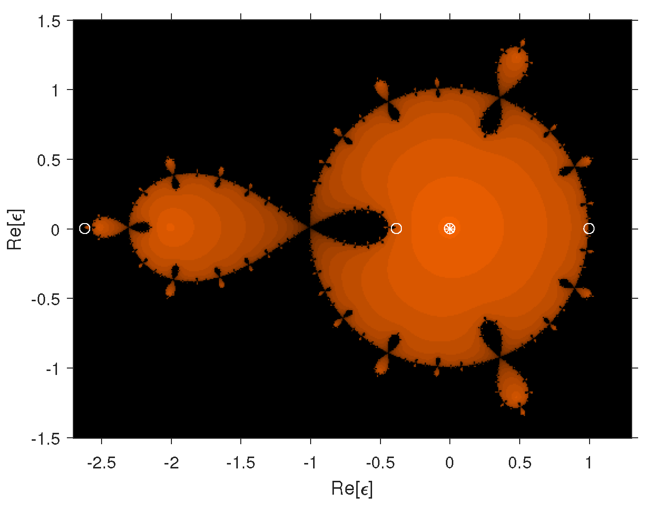
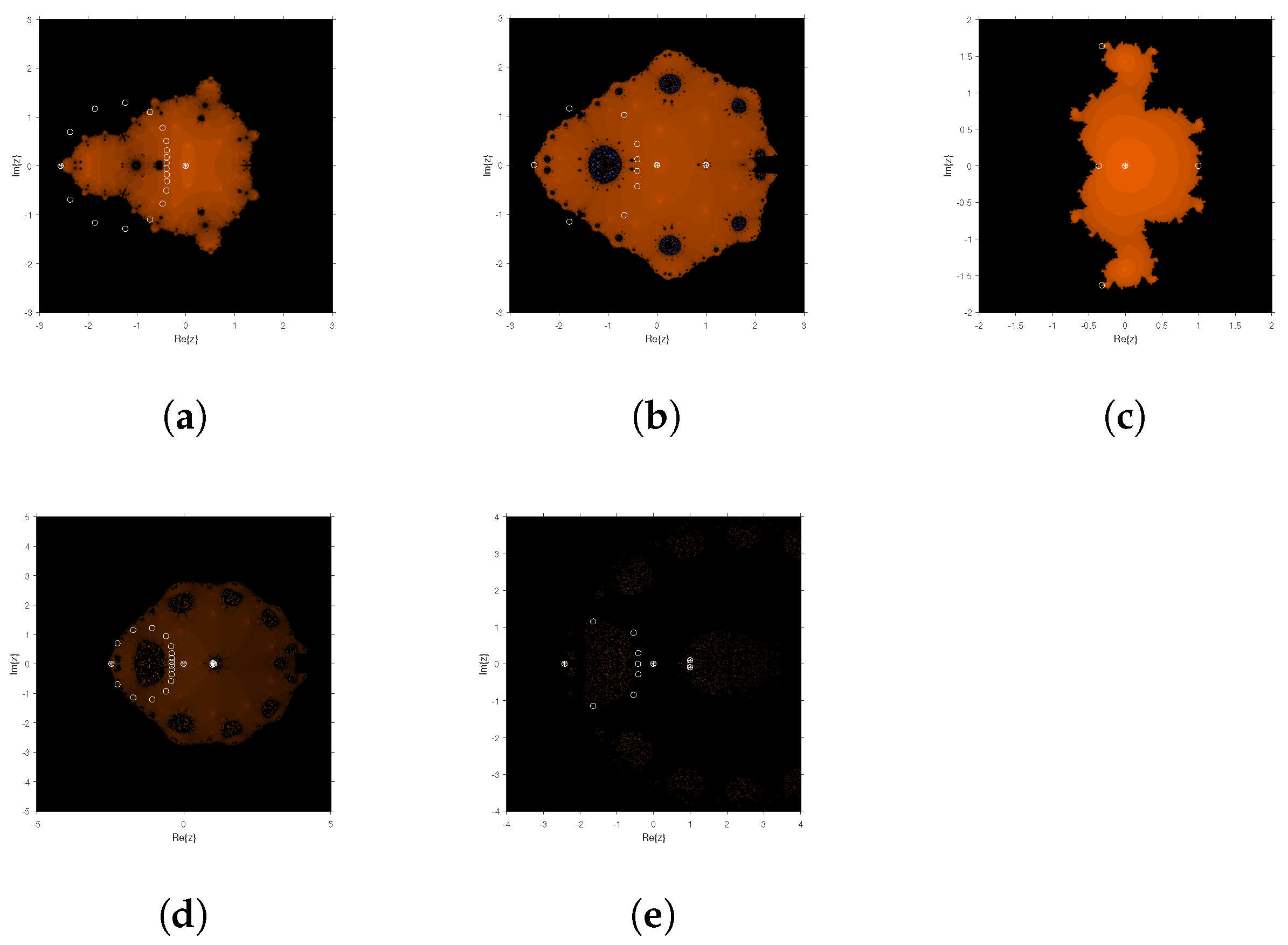
The dynamical planes in iterative methods are essential for solving nonlinear equations because they provide visual insights into the behavior and stability of iterating processes. By investigating the convergence and divergence patterns within these planes, fixed points, attractors, and chaotic zones can be identified, allowing the iterative process to be optimized for improved accuracy and efficiency. The stability of the single root-finding method for different fractional parameter values $\psi \in \left[0,1\right]$ is examined using dynamical planes (see Figure 1 and Figure 2). In these figures, the orange color represents the basins of attraction of $\mathrm{O}\left(x\right)$ when mapped to 0. If the root of $\mathrm{O}\left(x\right)$ maps to infinity, it is marked in blue. If the map diverges, it is marked in black. Strange fixed points are depicted by white circles, free critical points by white squares, and fixed points by white squares with a star. The dynamical planes are generated by taking starting values from the square $[-1.3,-1.3]\times [-1.3,1.3]$. In Figure 1, the dynamical planes show large basins where the rational map converges to 0 or infinity. In Figure 2a–e, the region of the basins of attraction decreases as the fractional parameter value decreases from 1 to 0.5 and diverges at 0. This indicates that the single-step method is more stable when the fractional parameter values are close to 1 and becomes unstable as the fractional parameter values approach 0. Using the newly developed stable fractional-order single root-finding method ${\mathrm{SCM}}^{\psi }$ as a correction factor in (23), we propose a novel inverse fractional scheme for analyzing (1) in the following section.

Figure 1. Dynamical planes of the rational map $\mathrm{O}\left(\epsilon \right)$ for $\psi \approx 1$.

Figure 2. (a–e): Dynamical planes for various parameter values of the rational map $\mathrm{O}\left(\epsilon \right)$. (a) Dynamical planes of the rational map $\mathrm{O}\left(\epsilon \right)$ for $\psi \approx 0.9$; (b) dynamical planes of the rational map $\mathrm{O}\left(\epsilon \right)$ for $\psi \approx 0.9$; (c) dynamical planes of the rational map $\mathrm{O}\left(\epsilon \right)$ for $\psi \approx 0.7$; (d) dynamical planes of the rational map $\mathrm{O}\left(\epsilon \right)$ for $\psi \approx 0.6$; (e) dynamical planes of the rational map $\mathrm{O}\left(\epsilon \right)$ for $\psi \approx 0.5$.

3. Development and Analysis of Inverse Fractional Parallel Scheme

The inverse fractional parallel iterative approach is useful for determining the roots of nonlinear equations because it efficiently finds all roots of (2) simultaneously. This iterative technique converges quickly from any initial value, has global convergence, and computes both real and complex roots simultaneously. The inverse fractional schemes provide greater stability, consistency and are well suited for parallel computing. Shams et al. [61] presented the fractional parallel approach with convergence order 2 for solving (2) as follows:

$$x_i^{\left[1+1\right]}={\displaystyle \frac{{\left(x_i^{\left[l\right]}\right)}^2\underset{\stackrel{j=1}{j\ne i}}{\stackrel{n}{\Pi }}\left(x_i^{\left[l\right]}-u_j^{\left[l\right]}\right)}{\left(x_i^{\left[l\right]}\right)\underset{\stackrel{j=1}{j\ne i}}{\stackrel{n}{\Pi }}\left(x_i^{\left[l\right]}-u_j^{\left[l\right]}\right)+g\left(x_i^{\left[l\right]}\right)}},$$

where $u_j^{\left[l\right]}=x_j^{\left[l\right]}-{\left(\Gamma (\psi +1){\displaystyle \frac{g\left(x_j^{\left[l\right]}\right)}{\left[{}_{\check{c}}ᘐ_{{\psi }_1}^{\psi }\right]g\left(x_j^{\left[l\right]}\right)}}\right)}^{1/\psi }.$ Using (4) in (23), we propose the following inverse fractional parallel scheme (${\mathrm{CSM}}^{\left[\psi \right]}$) as

$$x_i^{\left[1+1\right]}=x_i^{\left[l\right]}-{\displaystyle \frac{w^{[\ast \ast ]}\left(x_i^{\left[l\right]}\right)}{1+\frac{w^{[\ast \ast ]}\left(x_i^{\left[l\right]}\right)}{x_i^{\left[l\right]}}}},$$

(39)

where $w^{[\ast \ast ]}\left(x_i^{\left[l\right]}\right)={\displaystyle \frac{1}{2}}\left[3-{\displaystyle \frac{w^{[\ast ]}\left(x_i^{\left[l\right]}\right)}{w\left({\varsigma }_i^{\left[1\right]}\right)}}{\displaystyle \frac{g\left({\varsigma }_i^{\left[1\right]}\right)}{g\left(x_i^{\left[l\right]}\right)}}\right]w^{[\ast ]}\left(x_i^{\left[l\right]}\right)$, ${\varsigma }_i^{\left[1\right]}=x_i^{\left[l\right]}-{\displaystyle \frac{w^{[\ast ]}\left(x_i^{\left[l\right]}\right)}{1+\frac{w^{[\ast ]}\left(x_i^{\left[l\right]}\right)}{x_i^{\left[l\right]}}}},w^{[\ast ]}\left(x_i^{\left[l\right]}\right)={\displaystyle \frac{g\left(x_j^{\left[l\right]}\right)}{\underset{\stackrel{j=1}{j\ne i}}{\stackrel{n}{\Pi }}\left(x_i^{\left[l\right]}-u_j^{\left[l\right]}\right)}}$, $u_j^{\left[l\right]}={\gamma }_j^{\left[l\right]}-{\left({\displaystyle \frac{1}{2}}\Gamma (\psi +1)\left(3-{\displaystyle \frac{\left[{}_{\check{c}}ᘐ_{{\psi }_1}^{\psi }\right]g\left({\varsigma }_j^{\left[l\right]}\right)}{\left[{}_{\check{c}}ᘐ_{{\psi }_1}^{\psi }\right]g\left(x_j^{\left[l\right]}\right)}}\right){\displaystyle \frac{g\left(x_j^{\left[l\right]}\right)}{\left[{}_{\check{c}}ᘐ_{{\psi }_1}^{\psi }\right]g\left(x_j^{\left[l\right]}\right)}}\right)}^{1/\psi }$, ${\varsigma }_j^{\left[l\right]}=x_j^{\left[l\right]}-{\left(\Gamma (\psi +1){\displaystyle \frac{g\left(x_j^{\left[l\right]}\right)}{\left[{}_{\check{c}}ᘐ_{{\psi }_1}^{\psi }\right]g\left(x_j^{\left[l\right]}\right)}}\right)}^{1/\psi }.$ The parallel fractional scheme can also be written as

$$x_i^{\left[1+1\right]}=x_i^{\left[l\right]}-{\displaystyle \frac{\left[\frac{1}{2}\left[3-\frac{\underset{\stackrel{j=1}{j\ne i}}{\stackrel{n}{\Pi }}\left({\varsigma }_i^{\left[l\right]}-{\varsigma }_j^{\left[l\right]}\right)}{\underset{\stackrel{j=1}{j\ne i}}{\stackrel{n}{\Pi }}\left(x_i^{\left[l\right]}-u_j^{\left[l\right]}\right)}\right]\frac{g\left(x_j^{\left[l\right]}\right)}{\underset{\stackrel{j=1}{j\ne i}}{\stackrel{n}{\Pi }}\left(x_i^{\left[l\right]}-u_j^{\left[l\right]}\right)}\right]}{1+\frac{\left[\frac{1}{2}\left[3-\frac{\underset{\stackrel{j=1}{j\ne i}}{\stackrel{n}{\Pi }}\left({\varsigma }_i^{\left[l\right]}-{\varsigma }_j^{\left[l\right]}\right)}{\underset{\stackrel{j=1}{j\ne i}}{\stackrel{n}{\Pi }}\left(x_i^{\left[l\right]}-u_j^{\left[l\right]}\right)}\right]\frac{g\left(x_j^{\left[l\right]}\right)}{\underset{\stackrel{j=1}{j\ne i}}{\stackrel{n}{\Pi }}\left(x_i^{\left[l\right]}-u_j^{\left[l\right]}\right)}\right]}{x_i^{\left[l\right]}}}},$$

(40)

where

$${\varsigma }_i^{\left[1\right]}=x_i^{\left[l\right]}-{\displaystyle \frac{\left[\frac{g\left(x_j^{\left[l\right]}\right)}{\underset{\stackrel{j=1}{j\ne i}}{\stackrel{n}{\Pi }}\left(x_i^{\left[l\right]}-u_j^{\left[l\right]}\right)}\right]}{1+\frac{\left[\frac{g\left(x_j^{\left[l\right]}\right)}{\underset{\stackrel{j=1}{j\ne i}}{\stackrel{n}{\Pi }}\left(x_i^{\left[l\right]}-u_j^{\left[l\right]}\right)}\right]}{x_i^{\left[l\right]}}}},$$

and

$$\left\{\begin{array}{c}{\varsigma }_j^{\left[l\right]}=x_j^{\left[l\right]}-{\left(\Gamma (\psi +1){\displaystyle \frac{g\left(x_j^{\left[l\right]}\right)}{\left[{}_{\check{c}}ᘐ_{{\psi }_1}^{\psi }\right]g\left(x_j^{\left[l\right]}\right)}}\right)}^{1/\psi },\\ u_j^{\left[l\right]}={\gamma }_j^{\left[l\right]}-{\left({\displaystyle \frac{1}{2}}\Gamma (\psi +1)\left(3-{\displaystyle \frac{\left[{}_{\check{c}}ᘐ_{{\psi }_1}^{\psi }\right]g\left({\varsigma }_j^{\left[l\right]}\right)}{\left[{}_{\check{c}}ᘐ_{{\psi }_1}^{\psi }\right]g\left(x_j^{\left[l\right]}\right)}}\right){\displaystyle \frac{g\left(x_j^{\left[l\right]}\right)}{\left[{}_{\check{c}}ᘐ_{{\psi }_1}^{\psi }\right]g\left(x_j^{\left[l\right]}\right)}}\right)}^{1/\psi }.\end{array}\right.$$

The following theorem presents the local order of convergence of the inverse fractional scheme.

Theorem  3.

Let ${\zeta }_1,\dots ,{\zeta }_{\sigma }$ be simple zeros of the nonlinear equation. For sufficiently close initial distinct estimates ${\epsilon }_1^{\left[0\right]},\dots ,{\epsilon }_n^{\left[0\right]}$ of the roots, respectively, ${\mathit{CIM}}^{\left[\psi \right]}$ has a convergence order of $2\psi +2$.

Proof. 

Let $e_i=x_i^{\left[l\right]}-{\zeta }_i,e_{\varsigma }={\varsigma }_i^{\left[l\right]}-{\zeta }_i,$ and $e_i^{[\ast ]}=x_i^{[l+1]}-{\zeta }_i$ be the errors in $x_i^{\left[l\right]}$, ${\varsigma }_i^{\left[l\right]},$ and $x_i^{[l+1]}$, respectively. From the first step of ${\mathrm{CSM}}^{\left[\psi \right]}$, we have

$${\varsigma }_i^{\left[l\right]}-{\zeta }_i=x_i^{\left[l\right]}-{\zeta }_i-{\displaystyle \frac{\left[\frac{g\left(x_j^{\left[l\right]}\right)}{\underset{\stackrel{j=1}{j\ne i}}{\stackrel{n}{\Pi }}\left(x_i^{\left[l\right]}-u_j^{\left[l\right]}\right)}\right]}{1+\frac{w^{[\ast ]}\left(x_i^{\left[l\right]}\right)}{x_i^{\left[l\right]}}}},$$

(41)

$$e_i^{\prime }=e_i-{\displaystyle \frac{e_i{\displaystyle \underset{\stackrel{j=1}{j\ne i}}{\prod ^n}}\left[\frac{x_i^{\left[l\right]}-{\zeta }_j}{x_i^{\left[l\right]}-u_j^{\left[l\right]}}\right]}{1+\frac{w^{[\ast ]}\left(x_i^{\left[l\right]}\right)}{x_i^{\left[l\right]}}}},$$

(42)

$$e_{\varsigma }=e_i\left(1-{\displaystyle \frac{{\displaystyle \underset{\stackrel{j=1}{j\ne i}}{\prod ^n}}\left[\frac{x_i^{\left[l\right]}-{\zeta }_j}{x_i^{\left[l\right]}-u_j^{\left[l\right]}}\right]}{1+\frac{w^{[\ast ]}\left(x_i^{\left[l\right]}\right)}{x_i^{\left[l\right]}}}}\right)=e_i\left({\displaystyle \frac{1-{\displaystyle \underset{\stackrel{j=1}{j\ne i}}{\prod ^n}}\left[\frac{x_i^{\left[l\right]}-{\zeta }_j}{x_i^{\left[l\right]}-u_j^{\left[l\right]}}\right]+\frac{w^{[\ast ]}\left(x_i^{\left[l\right]}\right)}{x_i^{\left[l\right]}}}{1+\frac{w^{[\ast ]}\left(x_i^{\left[l\right]}\right)}{x_i^{\left[l\right]}}}}\right),$$

(43)

$$e_{\varsigma }=e_i\left({\displaystyle \frac{1-{\displaystyle \underset{\stackrel{j=1}{j\ne i}}{\prod ^n}}\left[\frac{x_i^{\left[l\right]}-{\zeta }_j}{x_i^{\left[l\right]}-u_j^{\left[l\right]}}\right]+\frac{u_i^{\left[l\right]}-{\zeta }_j}{x_i^{\left[l\right]}}{\displaystyle \underset{\stackrel{j=1}{j\ne i}}{\prod ^n}}\left[\frac{u_i^{\left[l\right]}-{\zeta }_j}{x_i^{\left[l\right]}-u_j^{\left[l\right]}}\right]}{1+\frac{w^{[\ast ]}\left(x_i^{\left[l\right]}\right)}{x_i^{\left[l\right]}}}}\right),$$

(44)

where ${\displaystyle \underset{\stackrel{j=1}{j\ne i}}{\prod ^n}}\left[{\displaystyle \frac{x_i^{\left[l\right]}-{\zeta }_j}{x_i^{\left[l\right]}-u_j^{\left[l\right]}}}\right]-1={\displaystyle \sum _{k\ne i}^n}\left({\displaystyle \frac{-}{x_i^{\left[l\right]}-u_j^{\left[l\right]}}}\right){\displaystyle \underset{j\ne i}{\prod ^{k-1}}}\left[{\displaystyle \frac{u_i^{\left[l\right]}-{\zeta }_j}{x_i^{\left[l\right]}-u_j^{\left[l\right]}}}\right]$ and from (27), $u_j^{\left[l\right]}-{\zeta }_j=O\left(\left|{\left[e_i\right]}^{2\psi +1}\right|\right)$. Therefore,

$$e_{\varsigma }=e_i\left({\displaystyle \frac{{\displaystyle \sum _{k\ne i}^n}\left(\frac{-e_i^{2\psi +1}}{x_i^{\left[l\right]}-u_j^{\left[l\right]}}\right){\displaystyle \underset{j\ne i}{\prod ^{k-1}}}\left[\frac{u_i^{\left[l\right]}-{\zeta }_j}{x_i^{\left[l\right]}-u_j^{\left[l\right]}}\right]+\frac{e_j^{2\psi +1}}{x_i^{\left[l\right]}}{\displaystyle \underset{\stackrel{j=1}{j\ne i}}{\prod ^n}}\left[\frac{u_i^{\left[l\right]}-{\zeta }_j}{x_i^{\left[l\right]}-u_j^{\left[l\right]}}\right]}{1+\frac{w^{[\ast ]}\left(x_i^{\left[l\right]}\right)}{x_i^{\left[l\right]}}}}\right),$$

(45)

By assuming $\left|e_i^{2\psi +1}\right|=\left|e_j^{2\psi +1}\right|,$

$$e_{\varsigma }=e_i\left(e_i^{2\psi +1}\right)\left({\displaystyle \frac{{\displaystyle \sum _{k\ne i}^n}\left(\frac{-e_i^{2\psi +1}}{x_i^{\left[l\right]}-u_j^{\left[l\right]}}\right){\displaystyle \underset{j\ne i}{\prod ^{k-1}}}\left[\frac{u_i^{\left[l\right]}-{\zeta }_j}{x_i^{\left[l\right]}-u_j^{\left[l\right]}}\right]+\frac{e_j^{2\psi +1}}{x_i^{\left[l\right]}}{\displaystyle \underset{\stackrel{j=1}{j\ne i}}{\prod ^n}}\left[\frac{u_i^{\left[l\right]}-{\zeta }_j}{x_i^{\left[l\right]}-u_j^{\left[l\right]}}\right]}{1+\frac{w^{[\ast ]}\left(x_i^{\left[l\right]}\right)}{x_i^{\left[l\right]}}}}\right),$$

(46)

$$e_{\varsigma }=O\left(e_i^{2\psi +2}\right).$$

(47)

Considering the second step, we have

$$x_i^{[l+1]}-{\zeta }_i=x_i^{\left[l\right]}-{\zeta }_i-{\displaystyle \frac{w^{[\ast \ast ]}\left(x_i^{\left[l\right]}\right)}{1+\frac{w^{[\ast \ast ]}\left(x_i^{\left[l\right]}\right)}{x_i^{\left[l\right]}}}},$$

(48)

$$e_i^{[\ast ]}=e_i-{\displaystyle \frac{w^{[\ast \ast ]}\left(x_i^{\left[l\right]}\right)}{1+\frac{w^{[\ast \ast ]}\left(x_i^{\left[l\right]}\right)}{x_i^{\left[l\right]}}}},$$

(49)

where $w^{[\ast \ast ]}\left(x_i^{\left[l\right]}\right)={\displaystyle \frac{1}{2}}\left[3-{\displaystyle \frac{w^{[\ast ]}\left(x_i^{\left[l\right]}\right)}{w\left({\varsigma }_i^{\left[1\right]}\right)}}{\displaystyle \frac{g\left({\varsigma }_i^{\left[1\right]}\right)}{g\left(x_i^{\left[l\right]}\right)}}\right]w^{[\ast ]}\left(x_i^{\left[l\right]}\right)$ and ${\displaystyle \frac{w^{[\ast ]}\left(x_i^{\left[l\right]}\right)}{w\left({\varsigma }_i^{\left[1\right]}\right)}}{\displaystyle \frac{g\left({\varsigma }_i^{\left[1\right]}\right)}{g\left(x_i^{\left[l\right]}\right)}}=1$ [1]. Therefore,

$$e_i^{[\ast ]}=e_i-{\displaystyle \frac{\frac{1}{2}\left[3-1\right]w^{[\ast ]}\left(x_i^{\left[l\right]}\right)}{1+\frac{\frac{1}{2}\left[3-1\right]w^{[\ast ]}\left(x_i^{\left[l\right]}\right)}{x_i^{\left[l\right]}}}},$$

(50)

$$e_i^{[\ast ]}=e_i-{\displaystyle \frac{w^{[\ast ]}\left(x_i^{\left[l\right]}\right)}{1+\frac{w^{[\ast ]}\left(x_i^{\left[l\right]}\right)}{x_i^{\left[l\right]}}}}=e_{\varsigma }=O\left(e_i^{2\psi +2}\right),$$

(51)

$$e_i^{[\ast ]}=O\left(e_i^{2\psi +2}\right).$$

(52)

Hence, the theorem is proven.    □

4. Numerical Results

To examine the effectiveness and stability of our proposed method, several engineering applications are analyzed in this section. In our experiments, we use the following termination criteria:

$$\left(i\right)e_i=∥x_i^{\left[1+1\right]}-x_i^{\left[1\right]}∥<{10}^{-32},$$

(53)

where $e_i$ represents the residual error norm-2. Additionally, for percentage convergence, we use

$$\mathrm{Per}\text{-}\mathrm{C}=∥\left({\displaystyle \frac{x_i^{\left[1+1\right]}-x_i^{\left[1\right]}}{x_i^{\left[1\right]}}}\right)\ast 100∥<{10}^{-32}.$$

(54)

Additionally, we measure the CPU execution time using an Intel(R) Core(TM) i7-4330m CPU running at 8.2 GHz with a 64-bit operating system. All computations are carried out in Maple 20 and C++ to determine the more realistic run time of the numerical approach for comparison. Further, we compare our newly developed method with the Nourien method [62] (${\mathrm{NSM}}^{\left[4\right]}$), which has a convergence order of four:

$$x_i^{\left[l+1\right]}=x_i^{\left[l\right]}-{\displaystyle \frac{w\left(x_i^{\left[l\right]}\right)}{1+{\displaystyle \sum _{\stackrel{j=1}{j\ne i}}^n}\left(\frac{w\left(x_j^{\left[l\right]}\right)}{\left(x_i^{\left[l\right]}-w\left(x_j^{\left[l\right]}\right)-x_j^{\left[l\right]}\right)}\right)}};$$

(55)

and the Zhang et al. method [63] (${\mathrm{ZSM}}^{\left[5\right]}$):

$$x_i^{\left[l+1\right]}=x_i^{\left[l\right]}-{\displaystyle \frac{w\left(x_i^{\left[l\right]}\right)}{1+{\Delta }^{[\ast ]}\left(x_i^{\left[l\right]}\right)+\sqrt{\begin{array}{c}{\left(1+{\Delta }^{[\ast ]}\left(x_i^{\left[l\right]}\right)\right)}^2+\\ 4w\left(x_i^{\left[l\right]}\right){\displaystyle \sum _{\stackrel{j=1}{j\ne i}}^n}\left(\frac{w\left(x_j^{\left[l\right]}\right)}{\left(x_i^{\left[l\right]}-x_j^{\left[l\right]}\right)\left(x_i^{\left[l\right]}-w\left(x_i^{\left[l\right]}\right)-x_j^{\left[l\right]}\right)}\right)\end{array}}}};$$

(56)

where ${\Delta }^{[\ast ]}\left(x_i^{\left[l\right]}\right)={\displaystyle \sum _{\stackrel{j=1}{j\ne i}}^n}\left({\displaystyle \frac{w\left(x_j^{\left[l\right]}\right)}{x_i^{\left[l\right]}-x_j^{\left[l\right]}}}\right).$

To compute all the roots of (2), we used the Algorithm 1 block diagram Figure 3, which depicts the flow chart of the inverse parallel scheme ${\mathrm{CSM}}^{\left[\psi \right]}$.

Algorithm 1: Fractional numerical scheme ${\mathrm{CSM}}^{\left[\psi \right]}$

$$\begin{array}{c}\hfill \left[\begin{array}{c}\mathrm{Given}\mathrm{initial}\mathrm{values}{x}_i^{\left[0\right]}(i=1,\dots ,N),\mathrm{tolerance}\in >0\mathrm{and}\mathrm{set}l=0\mathrm{for}\mathrm{iterations}qq\\ \left[\begin{array}{c}\mathrm{Compute}:\left\{\begin{array}{c}{\varsigma }_j^{\left[l\right]}=x_j^{\left[l\right]}-{\left(\Gamma (\psi +1){\displaystyle \frac{g\left(x_j^{\left[l\right]}\right)}{\left[{}_{\check{c}}ᘐ_{{\psi }_1}^{\psi }\right]g\left(x_j^{\left[l\right]}\right)}}\right)}^{1/\psi }\\ u_j^{\left[l\right]}={\gamma }_j^{\left[l\right]}-{\left({\displaystyle \frac{1}{2}}\Gamma (\psi +1)\left(3-{\displaystyle \frac{\left[{}_{\check{c}}ᘐ_{{\psi }_1}^{\psi }\right]g\left({\varsigma }_j^{\left[l\right]}\right)}{\left[{}_{\check{c}}ᘐ_{{\psi }_1}^{\psi }\right]g\left(x_j^{\left[l\right]}\right)}}\right){\displaystyle \frac{g\left(x_j^{\left[l\right]}\right)}{\left[{}_{\check{c}}ᘐ_{{\psi }_1}^{\psi }\right]g\left(x_j^{\left[l\right]}\right)}}\right)}^{1/\psi },\end{array}\right..\\ \mathrm{Update}\left\{\begin{array}{c}{\varsigma }_i^{\left[1\right]}=x_i^{\left[l\right]}-{\displaystyle \frac{\left[\frac{g\left(x_j^{\left[l\right]}\right)}{\underset{\stackrel{j=1}{j\ne i}}{\stackrel{n}{\Pi }}\left(x_i^{\left[l\right]}-u_j^{\left[l\right]}\right)}\right]}{1+\frac{\left[\frac{g\left(x_j^{\left[l\right]}\right)}{\underset{\stackrel{j=1}{j\ne i}}{\stackrel{n}{\Pi }}\left(x_i^{\left[l\right]}-u_j^{\left[l\right]}\right)}\right]}{x_i^{\left[l\right]}}}}\\ x_i^{\left[1+1\right]}=x_i^{\left[l\right]}-{\displaystyle \frac{\left[\frac{1}{2}\left[3-\frac{\underset{\stackrel{j=1}{j\ne i}}{\stackrel{n}{\Pi }}\left({\varsigma }_i^{\left[l\right]}-{\varsigma }_j^{\left[l\right]}\right)}{\underset{\stackrel{j=1}{j\ne i}}{\stackrel{n}{\Pi }}\left(x_i^{\left[l\right]}-u_j^{\left[l\right]}\right)}\right]\frac{g\left(x_j^{\left[l\right]}\right)}{\underset{\stackrel{j=1}{j\ne i}}{\stackrel{n}{\Pi }}\left(x_i^{\left[l\right]}-u_j^{\left[l\right]}\right)}\right]}{1+\frac{\left[\frac{1}{2}\left[3-\frac{\underset{\stackrel{j=1}{j\ne i}}{\stackrel{n}{\Pi }}\left({\varsigma }_i^{\left[l\right]}-{\varsigma }_j^{\left[l\right]}\right)}{\underset{\stackrel{j=1}{j\ne i}}{\stackrel{n}{\Pi }}\left(x_i^{\left[l\right]}-u_j^{\left[l\right]}\right)}\right]\frac{g\left(x_j^{\left[l\right]}\right)}{\underset{\stackrel{j=1}{j\ne i}}{\stackrel{n}{\Pi }}\left(x_i^{\left[l\right]}-u_j^{\left[l\right]}\right)}\right]}{x_i^{\left[l\right]}}}},\end{array}\right.\\ x_i^{\left[1+1\right]}=x_i^{\left[l\right]}(i=1,\dots ,n).\\ \mathrm{if}{e}_i^{\left[l\right]}=∥x_i^{\left[1+1\right]}-x_i^{\left[1\right]}∥<{10}^{-32}<\in ={10}^{-30}\mathrm{or}\sigma >pp,\mathrm{then}\mathrm{stop}.\end{array}\right.\\ \mathrm{Set}l=l+1\mathrm{and}\mathrm{go}\mathrm{to}\mathrm{step}2.\\ \mathrm{End}\mathrm{do}.\end{array}\right.\end{array}$$

Figure 3. Flow chart of the inverse parallel scheme ${\mathrm{CSM}}^{\left[\psi \right]}$ for solving (2).

4.1. Example 1: Fractional Relaxation–Oscillation Equation [64]

A fundamental tool for forecasting the dynamic behavior of systems exhibiting both relaxation and oscillatory properties is the fractional relaxation–oscillation equation. This equation has applications in materials science, engineering, and biology, as it incorporates fractional derivatives that account for the system’s memory and hereditary effects, extending traditional relaxation–oscillation models. The fractional relaxation–oscillation equation is given by

$$\left\{\begin{array}{c}{}_{\check{c}}ᘐ_{{\psi }_1}^{n\psi }g\left(x\right)+{\vartheta }^{[\ast ]}g\left(x\right)=f\left(x\right);{ϵ}_0\le x\le {ϵ}_n\\ g^{(n-1)\psi }\left({ϵ}_0\right)={\theta }_{n-1}^{[\ast ]},\dots ,g\left({ϵ}_0\right)={\theta }_0^{[\ast ]}\end{array}\right..$$

(57)

In viscoelastic materials with both elastic and viscous behavior, the fractional order $\psi$ explains how the material’s stress response is influenced by its current state and deformation history.

The numerical solution of (57) can be obtained by solving the following polynomial, using the approach described in [65]. For this example, we choose $n=2,{\vartheta }^{[\ast ]}=0$, ${\theta }_0^{[\ast ]}=0$, ${\theta }_{n-1}^{[\ast ]}=1$, and $f\left(x\right)=g^2\left(x\right)+1$:

$$g\left(x\right)={\displaystyle \frac{x^{\psi }}{\Gamma (1+\psi )}}+{\displaystyle \frac{x^{2\psi }}{\Gamma (1+2\psi )}}+{\displaystyle \frac{2x^{4\psi }}{\Gamma (1+4\psi )}}+{\displaystyle \frac{6x^{5\psi }}{\Gamma (1+5\psi )}}+{\displaystyle \frac{6x^{6\psi }}{\Gamma (1+6\psi )}}.$$

(58)

For $\psi =1,$ this simplifies to

$$g\left(x\right)={\displaystyle \frac{x}{\Gamma \left(2\right)}}+{\displaystyle \frac{x^2}{\Gamma \left(3\right)}}+{\displaystyle \frac{2x^4}{\Gamma \left(5\right)}}+{\displaystyle \frac{6x^5}{\Gamma \left(6\right)}}+{\displaystyle \frac{6x^6}{\Gamma \left(7\right)}},$$

(59)

The Caputo-type derivative of Equation (58) is given by

$$\left[{}_{\check{c}}ᘐ_{{\psi }_1}^{\psi }\right]g\left(x\right)=\left[\begin{array}{c}{\displaystyle \frac{6}{\Gamma (7-\psi )}}{x}^{6-\psi }+{\displaystyle \frac{6}{\Gamma (6-\psi )}}{x}^{5-\psi }+{\displaystyle \frac{2}{\Gamma (5-\psi )}}{x}^{4-\psi }+\\ {\displaystyle \frac{1}{\Gamma (3-\psi )}}{x}^{2-\psi }+{\displaystyle \frac{1}{\Gamma (2-\psi )}}{x}^{1-\psi }\end{array}\right]$$

(60)

The non-linear Equation (58) has the following exact roots, accurate up to five decimal places:

$$\begin{array}{ccc}\hfill {\zeta }_{1,2}& =& -3.35615\pm 1.79321i,{\zeta }_3=-1.76807,{\zeta }_4=0.0,\hfill \\ \hfill {\zeta }_{5,6}& =& 1.24019\pm 1.77462i,\hfill \end{array}$$

Using initial guesses close to the exact solution, the convergence rate of simultaneous methods increases, allowing the methods to approach the exact roots with fewer iterations (see Table 1).

Table 1. Numerical results for Example 1.

Err	${\mathrm{ZSM}}^{\left[5\right]}$	${\mathrm{NSM}}^{\left[4\right]}$	${\mathrm{CSM}}^{\left[\mathit{\psi }\right]}$
$e_1^{\left[4\right]}$	$9.31\times {10}^{-45}$	$9.92\times {10}^{-99}$	$1.1\times {10}^{-104}$
$e_2^{\left[4\right]}$	$3.69\times {10}^{-55}$	$4.72\times {10}^{-76}$	$0.0$
$e_3^{\left[4\right]}$	$2.77\times {10}^{-76}$	$5.12\times {10}^{-85}$	$0.0$
$e_4^{\left[4\right]}$	$4.47\times {10}^{-39}$	$6.27\times {10}^{-101}$	$4.9\times {10}^{-165}$
$e_5^{\left[4\right]}$	$2.77\times {10}^{-76}$	$5.12\times {10}^{-85}$	$0.0$
$e_6^{\left[4\right]}$	$4.47\times {10}^{-39}$	$6.27\times {10}^{-101}$	$4.9\times {10}^{-165}$
${\sigma }_i^{[n-1]}$	0.05231	0.03794	0.01533

Table 2 clearly indicates that when $\psi \approx 1.0$, the residual error for each root and the order and rate of convergence are superior compared to existing methods, demonstrating better efficiency and stability. To observe the global convergence behavior, we selected some random initial guess values using the “rand()” command in Matlab to generate random initial guesses. The numerical outcomes for these random initial guesses are presented in Table 2.

Table 2. Random initial test vectors ${\mathrm{T}}_1^{[\ast ]}$ − ${\mathrm{T}}_3^{[\ast ]}$ for scheme ${\mathrm{CSM}}^{\left[\psi \right]}$.

Err	${\mathrm{T}}_1^{[\ast ]}$	${\mathrm{T}}_2^{[\ast ]}$	${\mathrm{T}}_3^{[\ast ]}$	${\mathrm{Ex-Sol}}^{\mathit{n}}$
$x_1^{\left[0\right]}$	$1.005+0.0078i$	$1.063+0.062i$	$1.013+0.0551i$	$-3.3652-1.7932i$
$x_2^{\left[0\right]}$	$2.001+1.342i$	$-2.03+1.054i$	$0.027+0.0139i$	$-3.3652+1.7932i$
$x_3^{\left[0\right]}$	$1.105+0.0078i$	$3.083+4.287i$	$5.013+0.432i$	$-1.76807$
$x_4^{\left[0\right]}$	$0.093+0.0018i$	$0.006+0.008i$	$8.019+0.051i$	$0.0$
$x_5^{\left[0\right]}$	$4.005+0.0044i$	$1.044+0.098i$	$4.013+0.091i$	$1.24019+1.77462i$
$x_6^{\left[0\right]}$	$2.012+0.0033i$	$2.063+0.106i$	$0.010+0.0331i$	$1.24019-1.77462i$

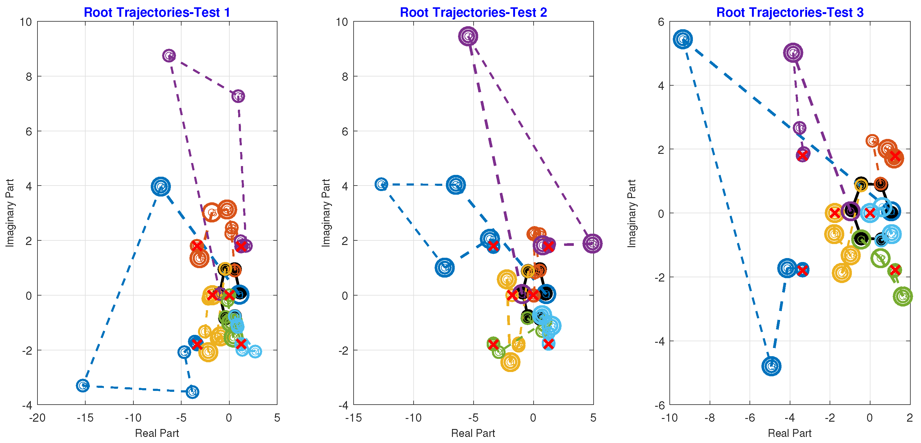
Root trajectories for roots 1–6 were determined by selecting random initial starting points using the Albearth initial approximation, with a maximum of 7, 8, 12, 10, and 12 iterations for $\psi \approx 1.0$ to converge to the exact roots. In Figure 4, the black solid circle represents the initial starting roots using the Albearth initial approximation, the empty circle shows the number of iterations required to reach the precise roots, and the red cross on the circle indicates the exact root’s position in the complex plane. The numerical technique converges to the exact roots, displaying global convergence characteristics for any collection of initial test problems, as demonstrated in Figure 4.

Figure 4. Root trajectories for all roots using three sets of test vectors.

Figure 5 clearly demonstrates that as we start with $\psi$ values of 0.1 and proceed closer to 1, the number of iterations decreases, indicating an increase in the convergence rate, which reaches its maximum as $\psi$ approaches 1. This is because the fractional derivative equals the ordinary derivative at $\psi =1$. The figure also illustrates that as $\psi$ increases from 0.1 to 0.9, the number of iterations decreases while accuracy increases, indicating that the newly developed approach becomes stable at $\psi \approx 1.0$. The scheme exhibits consistent behavior across all initial approximations, demonstrating global convergence and holding a prominent position in comparison to ${\mathrm{ZSM}}^{\left[5\right]}$ and ${\mathrm{NSM}}^{\left[4\right]}$.

Figure 5. Residual error of the numerical technique for different fractional parameter values and computational orders of convergence.

The global convergence behavior of the numerical scheme for different sets of random starting vectors is investigated in Table 2, Table 3 and Table 4. Random sets of starting values, using the Albearth initial approximation, are presented in Table 2 to find all solutions to the considered application. The comparisons of the starting vectors with exact roots up to four decimal places are shown in the last column. Table 3 presents the numerical outputs for various fractional parameter $\psi$ values ranging from 0.1 to 0.9 when these three initial vectors are used to find all solutions. As shown in Table 3, accuracy increases and reaches a maximum at $\psi \approx 1.0$ as the $\psi$ values increase from 0.1 to 0.9. To obtain this accuracy for different test vectors ${\mathrm{T}}_1^{\left[\psi \right]}$ − ${\mathrm{T}}_3^{\left[\psi \right]}$, the method requires a varying number of iterations for $\psi$, as shown in Table 4. It is also evident from Table 4 that the number of iterations decreases as $\psi$ increases from 0.1 to 0.9. Table 5 shows the scheme’s overall behavior with different sets of starting vectors.

Table 3. Residual error on random initial vectors for solving ${\mathrm{FDE}}^{\left[1\right]}$ using fractional ${\mathrm{CSM}}^{\left[\psi \right]}$ for different values of $\psi$.

$\mathit{\psi }$	${\mathit{e}}_1^{\left[\mathit{i}\right]}$	${\mathit{e}}_2^{\left[\mathit{i}\right]}$	${\mathit{e}}_3^{\left[\mathit{i}\right]}$	${\mathit{e}}_4^{\left[\mathit{i}\right]}$	${\mathit{e}}_5^{\left[\mathit{i}\right]}$	${\mathit{e}}_5^{\left[\mathit{i}\right]}$
0.1	$0.2\times {10}^{-5}$	$0.2\times {10}^{-5}$	$0.2\times {10}^{-5}$	$0.2\times {10}^{-5}$	$0.2\times {10}^{-5}$	$0.2\times {10}^{-5}$
0.2	$1.4\times {10}^{-6}$	$1.4\times {10}^{-6}$	$1.4\times {10}^{-6}$	$1.4\times {10}^{-6}$	$1.4\times {10}^{-6}$	$1.4\times {10}^{-6}$
0.3	$0.7\times {10}^{-6}$	$0.7\times {10}^{-6}$	$0.7\times {10}^{-6}$	$0.7\times {10}^{-6}$	$0.7\times {10}^{-6}$	$0.7\times {10}^{-6}$
0.4	$0.5\times {10}^{-4}$	$0.5\times {10}^{-4}$	$0.5\times {10}^{-4}$	$0.5\times {10}^{-4}$	$0.5\times {10}^{-4}$	$0.5\times {10}^{-4}$
0.5	$5.4\times {10}^{-6}$	$5.4\times {10}^{-6}$	$5.4\times {10}^{-6}$	$5.4\times {10}^{-6}$	$5.4\times {10}^{-6}$	$5.4\times {10}^{-6}$
0.6	$1.3\times {10}^{-7}$	$1.3\times {10}^{-7}$	$1.3\times {10}^{-7}$	$1.3\times {10}^{-7}$	$1.3\times {10}^{-7}$	$1.3\times {10}^{-7}$
0.7	$0.6\times {10}^{-9}$	$0.6\times {10}^{-9}$	$0.6\times {10}^{-9}$	$0.6\times {10}^{-9}$	$0.6\times {10}^{-9}$	$0.6\times {10}^{-9}$
0.8	$0.3\times {10}^{-11}$	$0.3\times {10}^{-11}$	$0.3\times {10}^{-11}$	$0.3\times {10}^{-11}$	$0.3\times {10}^{-11}$	$0.3\times {10}^{-11}$
0.9	$2.6\times {10}^{-16}$	$2.6\times {10}^{-16}$	$2.6\times {10}^{-16}$	$2.6\times {10}^{-16}$	$2.6\times {10}^{-16}$	$2.6\times {10}^{-16}$

Table 4. Number of iterations for random initial test vectors for solving engineering application 1 using ${\mathrm{CSM}}^{\left[\psi \right]}$.

$\mathit{\psi }$	${\mathit{e}}_1^{\left[\mathit{i}\right]}$	${\mathit{e}}_2^{\left[\mathit{i}\right]}$	${\mathit{e}}_3^{\left[\mathit{i}\right]}$	${\mathit{e}}_4^{\left[\mathit{i}\right]}$	${\mathit{e}}_5^{\left[\mathit{i}\right]}$	${\mathit{e}}_6^{\left[\mathit{i}\right]}$
0.1	7	8	12	11	10	12
0.2	8	8	11	7	7	11
0.3	8	7	8	6	8	10
0.4	7	8	8	7	7	9
0.5	6	7	9	6	6	9
0.6	9	7	7	8	6	7
0.7	7	5	7	9	6	8
0.8	6	8	7	7	7	6
0.9	5	5	5	7	7	5

Table 5. Consistency analysis for different $\psi$ values for solving engineering application 1 as described in Example 1.

$\mathit{\psi }$	${\mathit{\sigma }}_{\mathit{i}}^{[\mathit{n}-1]}$	Per-C	Av-it	CPU
$0.1$	$1.1222423$	$31.001$	05	$0.09378$
$0.2$	$1.5234264$	$37.0234$	05	$0.08637$
$0.3$	$1.9874325$	$38.0283$	06	$0.08386$
$0.4$	$2.4574334$	$39.0082$	06	$0.07647$
$0.5$	$2.8796536$	$45.1093$	05	$0.06435$
$0.6$	$2.9994356$	$55.0072$	06	$0.06343$
$0.7$	$3.0034287$	$59.0041$	06	$0.05535$
$0.8$	$3.6785857$	$60.5632$	05	$0.02844$
$0.9$	$4.0123332$	899823	05	$0.00138$

To determine the degree of consistency between the method and other existing methods, Table 5 is utilized. Table 5 assesses the method’s consistency with other existing methods, specifically ${\mathrm{ZSM}}^{\left[5\right]}$ and ${\mathrm{NSM}}^{\left[4\right]}$. Table 5 shows that ${\sigma }_i^{[n-1]}$ is the computational order of convergence, CPU is the average CPU time using various sets of initial vectors (${\mathrm{T}}_1^{\left[\psi \right]}$ − ${\mathrm{T}}_3^{\left[\psi \right]}$), Av-it is the average number of iterations, and Per-C is the percentage average. Comparing the results for $\psi \approx 1.0$ with the outcomes presented in Table 1 clearly shows that the method is more consistent compared to existing methods and demonstrates improved convergence behavior of ${\mathrm{CSM}}^{\left[\psi \right]}$ compared to ${\mathrm{ZSM}}^{\left[5\right]}$ and ${\mathrm{NSM}}^{\left[4\right]}$.

4.2. Example 2: Civil Engineering Application [66]

Consider the fractional differential equations

$$\left\{\begin{array}{c}{}_{\check{c}}ᘐ_{{\psi }_1}^{n\psi }g\left(x\right)+e^{-2g\left(x\right)}=0;1\le \psi \le 2\\ y\left(0\right)={\theta }_0^{[\ast ]},\dots ,g^{\prime }\left({ϵ}_0\right)={\theta }_{n-1}^{[\ast ]}\end{array}\right.$$

(61)

In viscoelastic materials with both elastic and viscous behavior, the fractional order $\psi$ explains how the material’s stress response is influenced by its current state and deformation history.

The numerical solution of (61) can be obtained by solving the following polynomial using the approach described in [67] by choosing ${\vartheta }^{[\ast ]}=0$ and ${\theta }_{n-1}^{[\ast ]}=1$:

$$g\left(x\right)=x+{\displaystyle \frac{-1}{\Gamma \left(\psi \right)}}\underset{0}{\stackrel{x}{\int }}{\left(x-s\right)}^{\psi -1}ds+{\displaystyle \frac{2}{\Gamma \left(\psi \right)}}\underset{0}{\stackrel{x}{\int }}{\left(x-s\right)}^{\psi -1}sds.$$

(62)

For $\psi =1.98,$ we have

$$g\left(x\right)=x-0.5092731905x^{{\displaystyle \frac{99}{50}}}+0.3417940876x^{{\displaystyle \frac{149}{50}}},$$

(63)

and for $\psi =2,$ we have

$$g\left(x\right)={\displaystyle \frac{1}{3}}{x}^3-{\displaystyle \frac{1}{2}}{x}^2-x.$$

(64)

The Caputo-type derivative of (63) is

$$\left[{}_{\check{c}}ᘐ_{{\psi }_1}^{\psi }\right]g\left(x\right)={\displaystyle \frac{1}{3}}{\displaystyle \frac{\Gamma \left(4\right)}{\Gamma (4-\psi )}}{x}^{3-\psi }+{\displaystyle \frac{1}{2}}{\displaystyle \frac{\Gamma \left(3\right)}{\Gamma (3-\psi )}}{x}^{2-\psi }-{\displaystyle \frac{\Gamma \left(2\right)}{\Gamma (2-\psi )}}{x}^{1-\psi }.$$

(65)

The non-linear equation (63) has the following exact roots up to three decimal places:

$${\zeta }_{1,2}=0.75\pm 1.56124i,{\zeta }_3=0.$$

Using initial guesses close to the exact solution, the convergence rate of simultaneous methods increases and approaches exact roots with fewer iterations, as shown in Table 6.

Table 6. Numerical results for Example 2.

Err	${\mathrm{ZSM}}^{\left[5\right]}$	${\mathrm{NSM}}^{\left[4\right]}$	${\mathrm{CSM}}^{\left[\mathit{\psi }\right]}$
$e_1^{\left[4\right]}$	$0.01\times {10}^{-55}$	$9.92\times {10}^{-109}$	$0.0$
$e_2^{\left[4\right]}$	$1.09\times {10}^{-25}$	$4.72\times {10}^{-86}$	$0.0$
$e_3^{\left[4\right]}$	$7.00\times {10}^{-76}$	$5.12\times {10}^{-95}$	$5.12\times {10}^{-195}$
${\sigma }_i^{[n-1]}$	0.0714	0.0518	0.0301

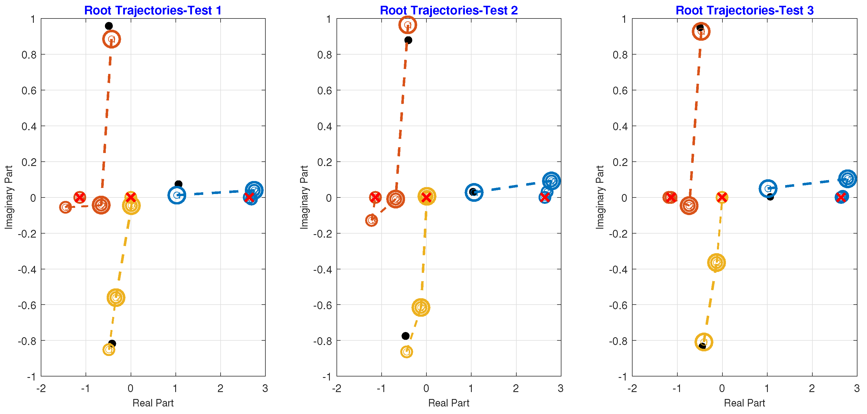
The root trajectories for roots 1 to 3 are determined by randomly selecting the initial starting values for each, using the Albearth approximation. This process requires a maximum of 7, 8, 12, 10, and 12 iterations for $\psi$ to converge to the precise root. The global convergence behavior of the numerical scheme is demonstrated by its consistent convergence to exact roots for any set of starting test problems ${\mathrm{T}}_1^{\left[\psi \right]}$ − ${\mathrm{T}}_3^{\left[\psi \right]}$, as depicted in Figure 6.

Figure 6. Root trajectories for all roots using three sets of test vectors.

Figure 7 clearly shows that as we start with $\psi$ values of 0.1 and move closer to 1, the number of iterations decreases. This indicates that the convergence rate increases and reaches a maximum as we approach $\psi =1$, since the fractional derivative equals the ordinary derivative at that value. The scheme exhibits consistent behavior across all initial approximations, demonstrating global convergence and maintaining a prominent position compared to current schemes, such as ${\mathrm{ZSM}}^{\left[5\right]}$ and ${\mathrm{NSM}}^{\left[4\right]}$.

Figure 7. Residual error of the numerical scheme for various fractional parameter values and computational orders of convergence.

The global convergence behavior of the numerical technique is examined in Table 7, Table 8 and Table 9 for various sets of random initial vectors. Using the Albearth initial approximation, random sets of starting values are generated to find all solutions to the specified application. These sets are displayed in Table 7. The last column compares the initial vectors with exact roots up to four decimal places. Table 8 presents the numerical outputs for fractional parameter values ranging from 0.1 to 0.9 when these three initial vectors are used to find all possible solutions. As $\psi$ values increase from 0.1 to 0.9, Table 8 demonstrates that accuracy rises and reaches a maximum at $\psi \approx 1.0$. To achieve this accuracy for different test vectors, the method requires a variable number of iterations for g, as shown in Table 9. Table 9 also clearly shows that the number of iterations decreases as $\psi$ grows from 0.1 to 0.9. Table 10 shows the scheme’s overall behavior with different sets of starting vectors.

Table 7. Random initial test vectors ${\mathrm{T}}_1^{\left[\psi \right]}$ − ${\mathrm{T}}_3^{\left[\psi \right]}$ for scheme ${\mathrm{CSM}}^{\left[\psi \right]}$.

Err	${\mathrm{T}}_1^{[\ast ]}$	${\mathrm{T}}_2^{[\ast ]}$	${\mathrm{T}}_3^{[\ast ]}$	${\mathrm{Ex-Sol}}^{\mathit{n}}$
$x_1^{\left[0\right]}$	$0.115+8.0078i$	$0.963+0.231i$	$4.015+6.0551i$	$0.75+1.56124i$
$x_2^{\left[0\right]}$	$6.005+3.1078i$	$5.051+0.002i$	$0.001+2.0431i$	$0.0$
$x_6^{\left[0\right]}$	$-1.05+0.0558i$	$0.081+6.012i$	$8.003+1.0051i$	$0.75-1.56124i$

Table 8. Residual error on random initial vectors for solving ${\mathrm{FDE}}^{\left[1\right]}$ using ${\mathrm{CSM}}^{\left[\psi \right]}$.

$\mathit{\psi }$	${\mathit{e}}_1^{\left[\mathit{i}\right]}$	${\mathit{e}}_2^{\left[\mathit{i}\right]}$	${\mathit{e}}_3^{\left[\mathit{i}\right]}$
0.1	$0.2\times {10}^{-5}$	$0.2\times {10}^{-5}$	$0.2\times {10}^{-5}$
0.2	$1.4\times {10}^{-6}$	$1.4\times {10}^{-6}$	$1.4\times {10}^{-6}$
0.3	$0.7\times {10}^{-6}$	$0.7\times {10}^{-6}$	$0.7\times {10}^{-6}$
0.4	$0.5\times {10}^{-4}$	$0.5\times {10}^{-4}$	$0.5\times {10}^{-4}$
0.5	$5.4\times {10}^{-6}$	$5.4\times {10}^{-6}$	$5.4\times {10}^{-6}$
0.6	$1.3\times {10}^{-7}$	$1.3\times {10}^{-7}$	$1.3\times {10}^{-7}$
0.7	$0.6\times {10}^{-9}$	$0.6\times {10}^{-9}$	$0.6\times {10}^{-9}$
0.8	$0.3\times {10}^{-11}$	$0.3\times {10}^{-11}$	$0.3\times {10}^{-11}$
0.9	$2.6\times {10}^{-16}$	$2.6\times {10}^{-16}$	$2.6\times {10}^{-16}$

Table 9. Number of iterations for random initial test vectors for solving engineering application 2.

$\mathit{\psi }$	${\mathit{e}}_1^{\left[\mathit{i}\right]}$	${\mathit{e}}_2^{\left[\mathit{i}\right]}$	${\mathit{e}}_3^{\left[\mathit{i}\right]}$	${\mathit{e}}_4^{\left[\mathit{i}\right]}$	${\mathit{e}}_5^{\left[\mathit{i}\right]}$	${\mathit{e}}_6^{\left[\mathit{i}\right]}$
0.1	7	8	12	11	10	12
0.2	8	8	11	7	7	11
0.3	8	7	8	6	8	10
0.4	7	8	8	7	7	9
0.5	6	7	9	6	6	9
0.6	9	7	7	8	6	7
0.7	7	5	7	9	6	8
0.8	6	8	7	7	7	6
0.9	5	5	5	7	7	5

Table 10. Consistancy analysis for different $\psi$ values for solving engineering application 2 using ${\mathrm{CSM}}^{\left[\psi \right]}$.

$\mathit{\psi }$	${\mathit{\sigma }}_{\mathit{i}}^{[\mathit{n}-1]}$	Per-C	Av-it	CPU
0.1	1.1222423	31.001	05	0.19378
0.2	1.5234264	37.0234	05	0.08937
0.3	1.9874325	38.0283	06	0.08086
0.4	2.4574334	39.0082	06	0.08665
0.5	2.8796536	45.1093	05	0.05535
0.6	2.9994356	55.0072	06	0.04443
0.7	3.0034287	59.0041	06	0.03535
0.8	3.6785857	60.5632	05	0.02844
0.9	4.0123332	899823	05	0.00138

It is evident from Table 10 that the method is more consistent than other approaches. The convergence behavior of ${\mathrm{CSM}}^{\left[\psi \right]}$ is superior to ${\mathrm{ZSM}}^{\left[5\right]}$, ${\mathrm{NSM}}^{\left[4\right]}$ when comparing the results for $\psi \approx 1.0$ with those shown in Table 10.

5. Conclusions

We developed a new Caputo-type fractional scheme with a convergence order of $2\psi +1$ and transformed it into an inverse fractional parallel scheme to find all solutions to nonlinear fractional problems. Convergence analysis reveals that the parallel schemes have a convergence order of $2\psi +2$. To enhance the convergence rate of fractional schemes, dynamical planes are utilized to select the optimal initial guessed values for convergence to exact solutions. Several nonlinear problems were considered to evaluate the stability and consistency of ${\mathrm{CSM}}^{\left[\psi \right]}$ in comparison to ${\mathrm{ZSM}}^{\left[5\right]}$, ${\mathrm{NSM}}^{\left[4\right]}$. The numerical results demonstrate that the ${\mathrm{CSM}}^{\left[\psi \right]}$ method is more stable and consistent in terms of residual error, CPU time, and error graphs for varied values of $\psi$ compared to ${\mathrm{ZSM}}^{\left[5\right]}$ and ${\mathrm{NSM}}^{\left[4\right]}$. The global convergence behavior is further examined using three initial test vectors, i.e., ${\mathrm{T}}_1^{\left[\psi \right]}$ − ${\mathrm{T}}_3^{\left[\psi \right]}$. In the future, we plan to develop higher-order inverse parallel schemes using other fractional derivative notations to address more complex problems in biomedical engineering and epidemic modeling.

References

1. Liu, Y.; Yang, Q. Dynamics of a new Lorenz-like chaotic system. Nonlinear Anal. Real World Appl. 2010, 11, 2563–2572. [Google Scholar] [CrossRef]
2. Liu, P.; Zhang, Y.; Mohammed, K.J.; Lopes, A.M.; Saberi-Nik, H. The global dynamics of a new fractional-order chaotic system. Chaos Solitons Fractals 2023, 175, 114006. [Google Scholar] [CrossRef]
3. Ye, X.; Wang, X. Hidden oscillation and chaotic sea in a novel 3d chaotic system with exponential function. Nonlinear Dyn. 2023, 111, 15477–15486. [Google Scholar] [CrossRef]
4. Venkateshan, S.P.; Swaminathan, P. Computational Methods in Engineering; Academic Press: Cambridge, MA, USA, 2014; pp. 317–373. [Google Scholar]
5. Hiptmair, R. Finite elements in computational electromagnetism. Acta Numer. 2002, 11, 237–339. [Google Scholar] [CrossRef]
6. Lomax, H.; Pulliam, T.H.; Zingg, D.W.; Kowalewski, T.A. Fundamentals of computational fluid dynamics. Appl. Mech. Rev. 2002, 55, B61. [Google Scholar] [CrossRef]
7. Warren, C.; Giannopoulos, A.; Giannakis, I. gprMax: Open source software to simulate electromagnetic wave propagation for Ground Penetrating Radar. Comput. Phys. Commun. 2016, 209, 163–170. [Google Scholar] [CrossRef]
8. Cantwell, B.J. Organized motion in turbulent flow. Annu. Rev. Fluid Mech. 1981, 13, 457–515. [Google Scholar] [CrossRef]
9. Peters, S.; Lanza, G.; Jun, N.; Xiaoning, J.; Pei Yun, Y.; Colledani, M. Automotive manufacturing technologies—An international viewpoint. Manuf. Rev. 2014, 1, 1–12. [Google Scholar] [CrossRef]
10. Singh, J.; Singh, H. Application of lean manufacturing in automotive manufacturing unit. Int. J. Lean Six Sigma 2020, 11, 171–210. [Google Scholar] [CrossRef]
11. Ma, C.Y.; Shiri, B.; Wu, G.C.; Baleanu, D. New fractional signal smoothing equations with short memory and variable order. Optik 2020, 218, 164507. [Google Scholar] [CrossRef]
12. Tolstoguzov, V. Phase behaviour of macromolecular components in biological and food systems. Food/Nahrung 2000, 44, 299–308. [Google Scholar] [CrossRef] [PubMed]
13. Bullmore, E.; Sporns, O. The economy of brain network organization. Nat. Rev. Neurosci. 2012, 13, 336–349. [Google Scholar] [CrossRef] [PubMed]
14. Arino, J.; Van den Driessche, P. Disease spread in metapopulations. Fields Inst. Commun. 2006, 4, 1–13. [Google Scholar]
15. Baleanu, D. Fractional Calculus: Models and Numerical Methods; World Scientific: Singapore, 2012; Volume 3. [Google Scholar]
16. Polyanin, A.D.; Zaitsev, V.F. Handbook of Ordinary Differential Equations: Exact Solutions, Methods, and Problems; Chapman and Hall/CRC: Boca Raton, FL, USA, 2017. [Google Scholar]
17. Diethelm, K.; Ford, N.J. Analysis of fractional differential equations. J. Math. Anal. Appl. 2002, 265, 229–248. [Google Scholar] [CrossRef]
18. Gu, X.M.; Huang, T.-Z.; Zhao, Y.L.; Carpentieri, B. A fast implicit difference scheme for solving the generalized time–space fractional diffusion equations with variable coefficients. Numer. Methods Partial. Differ. Equ. 2021, 37, 1136–1162. [Google Scholar] [CrossRef]
19. Gu, X.M.; Huang, T.Z.; Ji, C.C.; Carpentieri, B.; Alikhanov, A.A. Fast iterative method with a second-order implicit difference scheme for time-space fractional convection–diffusion equation. J. Sci. Comput. 2017, 72, 957–985. [Google Scholar] [CrossRef]
20. Huang, Y.Y.; Gu, X.M.; Gong, Y.; Li, H.; Zhao, Y.L.; Carpentieri, B. A fast preconditioned semi-implicit difference scheme for strongly nonlinear space-fractional diffusion equations. Fractal Fract. 2021, 5, 230. [Google Scholar] [CrossRef]
21. Karaagac, B. New exact solutions for some fractional order differential equations via improved sub-equation method. Discret. Contin. Dyn. Syst.-S 2019, 12, 447–454. [Google Scholar] [CrossRef]
22. Manafian, J.; Allahverdiyeva, N. An analytical analysis to solve the fractional differential equations. Adv. Math. Models Appl. 2021, 6, 128–161. [Google Scholar]
23. Qazza, A.; Saadeh, R. On the analytical solution of fractional SIR epidemic model. Appl. Comput. Intell. Soft Comput. 2023, 2023, 6973734. [Google Scholar] [CrossRef]
24. Yépez-Martínez, H.; Rezazadeh, H.; Inc, M.; Akinlar, M.A.; Gomez-Aguilar, J.F. Analytical solutions to the fractional Lakshmanan–Porsezian–Daniel model. Opt. Quantum Electron. 2022, 54, 32. [Google Scholar] [CrossRef]
25. Reynolds, D.R.; Gardner, D.J.; Woodward, C.S.; Chinomona, R. ARKODE: A flexible IVP solver infrastructure for one-step methods. ACM Trans. Math. Soft. 2023, 49, 1–26. [Google Scholar] [CrossRef]
26. Ikhile, M.N.O. Coefficients for studying one-step rational schemes for IVPs in ODEs: III. Extrapolation methods. Comput. Math. Appl. 2004, 47, 1463–1475. [Google Scholar] [CrossRef]
27. Rufai, M.A.; Ramos, H. A variable step-size fourth-derivative hybrid block strategy for integrating third-order IVPs, with applications. Int. J. Comput. Math. 2022, 99, 292–308. [Google Scholar] [CrossRef]
28. Argyros, I.K.; Hilout, S. Weaker conditions for the convergence of Newton’s method. J. Complex. 2012, 28, 364–387. [Google Scholar] [CrossRef]
29. Gutierrez, J.M.; Hernández, M.A. An acceleration of Newton’s method: Super-Halley method. Appl Math Comput. 2001, 117, 223–239. [Google Scholar] [CrossRef]
30. Chun, C. A new iterative method for solving nonlinear equations. Appl. Math. Comput. 2006, 178, 415–422. [Google Scholar] [CrossRef]
31. Sharma, J.R.; Guha, R.K. A family of modified Ostrowski methods with accelerated sixth order convergence. Appl. Math. Comput. 2007, 190, 111–115. [Google Scholar] [CrossRef]
32. King, P.R. The use of field theoretic methods for the study of flow in a heterogeneous porous medium. J. Phys. A Math. Gen. 1987, 20, 3935. [Google Scholar] [CrossRef]
33. Shams, M.; Carpentieri, B. On highly efficient fractional numerical method for solving nonlinear engineering models. Mathematics 2023, 11, 4914. [Google Scholar] [CrossRef]
34. Cordero, A.; Hueso, J.L.; MartÃ-nez, E.; Torregrosa, J.R. Increasing the convergence order of an iterative method for nonlinear systems. Appl. Math. Lett. 2012, 25, 2369–2374. [Google Scholar] [CrossRef]
35. Mir, N.A.; Anwar, M.; Shams, M.; Rafiq, N.; Akram, S. On numerical schemes for determination of all roots simultaneously of non-linear equation. Mehran Univ. Res. J. Eng. Technol. 2022, 41, 208–218. [Google Scholar] [CrossRef]
36. Akram, S.; Shams, M.; Rafiq, N.; Mir, N.A. On the stability of Weierstrass type method with King’s correction for finding all roots of non-linear function with engineering application. Appl. Math. Sci. 2020, 14, 461–473. [Google Scholar] [CrossRef]
37. Neta, B. New third order nonlinear solvers for multiple roots. Appl. Math. Comput. 2008, 202, 162–170. [Google Scholar] [CrossRef]
38. Amat, S.; Busquier, S.; Gutiérrez, J.M. Third-order iterative methods with applications to Hammerstein equations: A unified approach. J. Comput. Appl. Math. 2011, 235, 2936–2943. [Google Scholar] [CrossRef]
39. Liu, Z.; Zheng, Q.; Zhao, P. A variant of Steffensen’s method of fourth-order convergence and its applications. Appl. Math. Comput. 2010, 216, 1978–1983. [Google Scholar] [CrossRef]
40. Torres-Hernandez, A.; Brambila-Paz, F. Sets of fractional operators and numerical estimation of the order of convergence of afamily of fractional fixed-point methods. Fractal Fract. 2021, 4, 240. [Google Scholar] [CrossRef]
41. Akgül, A.; Cordero, A.; Torregrosa, J.R. A fractional Newton method with 2th-order of convergence and its stability. Appl. Math. Lett. 2019, 98, 344–351. [Google Scholar] [CrossRef]
42. Cajori, F. Historical note on the Newton-Raphson method of approximation. Am. Math. Mon. 1911, 18, 29–32. [Google Scholar] [CrossRef]
43. Kumar, P.; Agrawal, O.P. An approximate method for numerical solution of fractional differential equations. Signal Process 2006, 86, 2602–2610. [Google Scholar] [CrossRef]
44. Falcão, M.I.; Miranda, F.; Severino, R.; Soares, M.J. Weierstrass method for quaternionic polynomial root-finding. Math. Methods Appl. Sci. 2018, 41, 423–437. [Google Scholar] [CrossRef]
45. Nedzhibov, G.H. Inverse Weierstrass-Durand-Kerner Iterative Method. Int. J. Appl. Math. 2013, 28, 1258–1264. [Google Scholar]
46. Shams, M.; Rafiq, N.; Ahmad, B.; Mir, N.A. Inverse numerical iterative technique for finding all roots of nonlinear equations with engineering applications. J. Math. 2021, 2021, 6643514. [Google Scholar] [CrossRef]
47. Iliev, A.I. A generalization of Obreshkoff-Ehrlich method for multiple roots of polynomial equations. arXiv 2001, arXiv:math/0104239. [Google Scholar]
48. Petković, M.S.; Petković, L.D.; Džunić, J. On an efficient method for the simultaneous approximation of polynomial multiple roots. Appl. Anal. Discret. Math. 2014, 1, 73–94. [Google Scholar] [CrossRef]
49. Sebah, P.; Gourdon, X. Introduction to the gamma function. Am. J. Sci. Res. 2002, 1, 2–18. [Google Scholar]
50. Almeida, R. A Caputo fractional derivative of a function with respect to another function. Commun. Nonlinear Sci. Numer. Simul. 2017, 44, 460–481. [Google Scholar] [CrossRef]
51. Odibat, Z.M.; Shawagfeh, N.T. Generalized Taylor’s formula. Appl. Math. Comput. 2007, 186, 286–293. [Google Scholar] [CrossRef]
52. Candelario, G.; Cordero, A.; Torregrosa, J.R.; Vassileva, M.P. An optimal and low computational cost fractional Newton-type method for solving nonlinear equations. Appl. Math. Lett. 2022, 124, 107650. [Google Scholar] [CrossRef]
53. Shams, M.; Kausar, N.; Agarwal, P.; Jain, S.; Salman, M.A.; Shah, M.A. On family of the Caputo-type fractional numerical scheme for solving polynomial equations. Appl. Math. Sci. Eng. 2023, 31, 2181959. [Google Scholar] [CrossRef]
54. Candelario, G.; Cordero, A.; Torregrosa, J.R. Multipoint fractional iterative methods with (2α+1) th-order of convergence for solving nonlinear problems. Mathematics 2020, 8, 452. [Google Scholar] [CrossRef]
55. Jarratt, P. Some fourth order multipoint iterative methods for solving equations. Math. Comput. 1966, 20, 434–437. [Google Scholar] [CrossRef]
56. Chicharro, F.I.; Cordero, A.; Garrido, N.; Torregrosa, J.R. Stability and applicability of iterative methods with memory. J. Math. Chem. 2019, 57, 1282–1300. [Google Scholar] [CrossRef]
57. Cordero, A.; Leonardo Sepúlveda, M.A.; Torregrosa, J.R. Dynamics and stability on a family of optimal fourth-order iterative methods. Algorithms 2022, 15, 387. [Google Scholar] [CrossRef]
58. Cordero, A.; Lotfi, T.; Khoshandi, A.; Torregrosa, J.R. An efficient Steffensen-like iterative method with memory. Bull. Math. Soc. Sci. Math. Roum. 2015, 1, 49–58. [Google Scholar]
59. Shams, M.; Ahmad Mir, N.; Rafiq, N.; Almatroud, A.O.; Akram, S. On dynamics of iterative techniques for nonlinear equation with applications in engineering. Math. Probl. Eng. 2020, 2020, 5853296. [Google Scholar] [CrossRef]
60. Campos, B.; Canela, J.; Vindel, P. Dynamics of Newton-like root finding methods. Numer. Alg. 2023, 93, 1453–1480. [Google Scholar] [CrossRef]
61. Shams, M.; Carpentieri, B. Efficient Inverse Fractional Neural Network-Based Simultaneous Schemes for Nonlinear Engineering Applications. Fractal Fract. 2023, 7, 849. [Google Scholar] [CrossRef]
62. Anourein, A.W.M. An improvement on two iteration methods for simultaneous determination of the zeros of a polynomial. Inter. J. Comput. Math. 1977, 6, 241–252. [Google Scholar] [CrossRef]
63. Zhang, X.; Peng, H.; Hu, G. A high order iteration formula for the simultaneous inclusion of polynomial zeros. Appl. Math. Comput. 2006, 179, 545–552. [Google Scholar] [CrossRef]
64. Wu, G.C. Adomian decomposition method for non-smooth initial value problems. Math. Comput. Model. 2018, 54, 2104–2108. [Google Scholar] [CrossRef]
65. Az-Zo’bi, E.A.; Qousini, M.M. Modified Adomian-Rach decomposition method for solving nonlinear time-dependent IVPs. Appl. Math. Sci. 2017, 11, 387–395. [Google Scholar] [CrossRef]
66. Khodabakhshi, N.; Mansour Vaezpour, S.; Baleanu, D. Numerical solutions of the initial value problem for fractional differential equations by modification of the Adomian decomposition method. Fract. Calc. Appl. 2014, 17, 382–400. [Google Scholar] [CrossRef]
67. Wazwaz, A.M.; Rach, R.; Bougoffa, L. Dual solutions for nonlinear boundary value problems by the Adomian decomposition method. Int. J. Numer. Meth. Heat. Fluid Flow 2016, 26, 2393–2409. [Google Scholar]
Figure 1. Dynamical planes of the rational map O ε for ψ 1 .
Axioms 13 00671 g001