Abstract
In this paper, we propose an alternative distribution to model count data exhibiting uni/bimodality. It arises as a weighted version of the beta-binomial distribution, which is defined by a parametric weight function that admits up to two modes for the resulting probability mass function. Like the baseline beta-binomial distribution, the proposed distribution performs well in modeling overdispersed binomial data. Structural properties of the new distribution are studied. Raw moments are derived, which are used to describe the dispersion behavior relative to the mean and the skewness behavior. Parameter estimation is carried out using the maximum likelihood method. A simulation study is conducted in order to illustrate the behavior of the estimators. Finally, two applications illustrating the usefulness of the proposal are presented.
Keywords:
beta-binomial distribution; bimodality; count data; maximum likelihood; moments; overdispersion MSC:
62E10; 62F10
1. Introduction
Count data represents the number of times a particular event occurs in an interval of time, space, or other unit of measurement. This type of data is commonly found in various areas, such as medicine, economics, and engineering, to name a few. For example, Böhning et al. [1] analyzed count data from a dental epidemiological study under the situation of additional zeros. Salman et al. [2] analyzed bankruptcy count data from Swedish small manufacturing firms with the aim of investigating the business failure risk factors of small manufacturing firms. Calabria et al. [3] analyzed the reliability of repairable systems from in-service failure count data.
There are many real-world scenarios where the probability of success in binomial experiments cannot be considered constant. For example, the probability of consuming alcohol across the 7 days of a particular week varies from one individual to another (see Alanko and Lemmens [4]). Considering a beta distribution for the probability of success in a binomial distribution (which gives rise to the beta-binomial distribution) is not overly restrictive since the beta distribution is very flexible in terms of the shapes of its probability density function.
A random variable X follows the beta-binomial distribution, denoted , if its probability mass function (p.m.f.) is given by
where , , is the beta function.
In Bayesian inference, the beta-binomial distribution is used to make predictions about the number of successes in future trials, taking into account the uncertainty in the estimate of the probability of success. In classical inference, the beta-binomial distribution can be used to model data with overdispersion in binomial experiments, i.e., when the observed variability is greater than that expected under a standard binomial distribution.
A review of the applicability and extensions of the beta-binomial distribution can be found in Wilcox [5]. The use of the beta-binomial distribution in the context of regression is discussed in Crowder [6]. Details on the estimation of the parameters of the beta-binomial distribution can be found in Tripathi et al. [7].
Regarding more recent applications of the beta-binomial distribution, several studies can be found in the literature. To name a few, Palm et al. [8] use the beta-binomial distribution in the formulation of the BBARMA (Beta-Binomial Autoregressive Moving Average) model, which can capture the temporal dynamics and autoregressive structure in count data. Chen et al. [9] use the beta-binomial distribution to propose a GARCH model that captures the variation in the number of new cases of cryptosporidiosis infection, obtaining a useful model for time series data that present bounded counts and high volatility. Jansen and Holling [10], under a Bayesian approach, use the beta-binomial distribution in the meta-analysis of rare events.
Although the beta-binomial distribution is applied in various real-world settings, its performance is not good when empirical distributions exhibit bimodality, i.e., when there are two modes or peaks in the empirical distributions. The presence of bimodality can be explained by the existence of two groups or subpopulations with unique characteristics or by the existence of latent variables that significantly influence the distribution of the population.
A very popular methodology in the literature to incorporate flexibility in terms of asymmetry and multimodality is related to the definition of weighted distributions proposed by Fisher [11] and Rao [12]. Suppose that X is a random variable with probability function . The weighted random variable has PDF
where is a nonnegative weight function and .
A particularly salient case of (2) is obtained when , which defines a length-biased distribution. These distributions arise naturally in applied fields, such as reliability and survival analysis, when individuals or mechanical units are sampled with unequal probability due to the experimental design or the existing unequal probability of detection.
On the other hand, it is possible to find in the literature weight functions that can lead to multimodality for the weighted distributions resulting from (2). For example, if ,, and is the pdf of the normal distribution with mean and variance , then (2) reduces to the family of bimodal distributions called the alpha-skew-normal distribution, see Elal-Olivero [13]. Based on the same weight function, Gómez-Déniz et al. [14] introduces a bimodal version of the Poisson distribution. Cortés et al. [15] propose a parametric weight function that involves a power function of exponent 4, which can lead to a probability function with up to three modes.
In this paper, we propose an extension of the beta-binomial distribution appropriate to fit overdispersed binomial data that may exhibit both unimodality and bimodality. The proposal arises from (2), using the weight function proposed by Elal-Olivero [13] under a beta-binomial baseline distribution. In this way, the new distribution is aimed at expanding the use of beta-binomial distributions to real-world scenarios where empirical distributions exhibit bimodality.
The remainder of the paper is organized as follows. In Section 2, we define the bimodal beta-binomial random variable and study some of its properties, such as the probability mass function, cumulative distribution function, and the raw moments. The latter are used to describe the behavior of the relative dispersion with respect to the mean and the skewness behavior of the distribution. In Section 3, parameter estimation for the new distribution using the maximum likelihood method is discussed. A simulation study is carried out to evaluate the behavior of the estimators. In Section 4, two application examples with real data are presented to illustrate the usefulness of the proposed distribution. Finally, concluding remarks are presented in Section 5.
2. Bimodal Beta-Binomial Distribution
In this section, we derive the new distribution and study some of its main properties.
2.1. Bimodal Beta-Binomial Random Variable
The following proposition presents the p.m.f. of the new distribution.
Proposition 1.
Let and be a parametric function given by
where
are the mean and variance of X, respectively. Then, the p.m.f. of the weighted random variable is
such that , and is the beta function.
Proof.
First, we observe that for all when and . Second, it can be seen that
In consequence, it is concluded that (3) is a valid p.m.f. □
Definition 1.
Let be a random variable with p.m.f. given in (3), then we say that follows a bimodal beta-binomial distribution. We denote this as .
The name given in Definition 1 to refer to the new distribution is based on the bimodal behavior that the p.m.f. can present. Figure 1 shows some plots of the p.m.f. of the bimodal beta-binomial distribution for different values of its parameters. In the figure, it can be seen that the BBB p.m.f can present a great variety of shapes depending on its parameters: monotonic shape, symmetric/asymmetric unimodal shape, bathtub shape, or asymmetric bimodal shape.
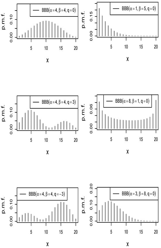
Figure 1.
Plots of the p.m.f. of the bimodal beta-binomial distribution with and different values of , and q.
2.2. Two Related Distributions
Corollary 1.
Let . Then,
- 1.
- , , , which is the p.m.f. of the beta-binomial distribution.
- 2.
- If , then , , such that
Corollary 1 is a direct consequence of (3) considering fixed values for q and n. Part 1 shows that the beta-binomial distribution is a special case of the bimodal beta-binomial distribution obtained when . The second part shows that the bimodal beta-binomial distribution reduces to the Bernoulli distribution with parameter , where is a function of the parameters , , and q.
2.3. Cumulative Distribution Function
The cumulative distribution function (c.d.f.) of can be obtained straightforwardly from Proposition 1.
Corollary 2.
Let . Then, the cumulative distribution function (c.d.f.) of is given by
where , .
Figure 2 shows some plots of the c.d.f. of the bimodal beta-binomial distribution for different values of , , and q. As expected, the figure shows that the frequencies are not decreasing as x increases. However, two sharp increases in frequency can be observed in two different intervals of x, which is explained by the bimodal behavior of the corresponding p.m.f.
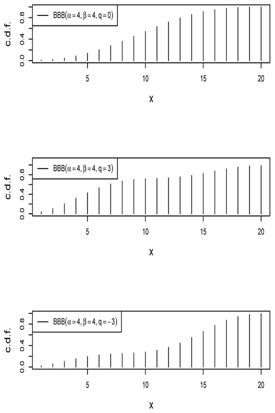
Figure 2.
Plots of the c.d.f. of the bimodal beta-binomial distribution with , , and different values of q.
A function in the R programming language for computing (4) is provided in Appendix A.
2.4. Moments
The following proposition derives the raw moments of the beta-binomial distribution. Essentially, these moments are expressed as a function of the raw moments of the beta-binomial distribution.
Proposition 2.
Let . Then, the rth raw moment of is given by
where
such that
is the j raw moment of the beta-binomial distribution.
Proof .
By definition of expectation, we have that
where is the p.m.f. of the beta-binomial distribution. Therefore, after some algebra, we see that
and the result is obtained by recognizing the raw moments of the beta-binomial distribution in the above expression. □
Alternatively, in (6) we can write , where . Then, using the binomial theorem, we have
Thus, we can write (7) as
where is the rth raw moment of the beta-binomial distribution.
Corollary 3.
Let . Then, the coefficient of variation () and the Fisher’s skewness coefficient () of are given by
where
such that a, b and c are as in Proposition 2 and
Figure 3 shows some curves of the coefficient of variation and the coefficient of skewness of the bimodal beta-binomial distribution as a function of q under fixed values for and . In the figure, it can be seen that the bimodal beta-binomial distribution (depending on q) can present a greater or lesser relative dispersion (and a greater or lesser skewness level) than the beta-binomial distribution (special case ).
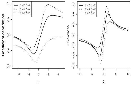
Figure 3.
Plots of the coefficient of variation and the skewness coefficient (as a function of q) of the bimodal beta-binomial distribution with and different values of and .
Functions in the R programming language for computing the rth moment (7) and for the coefficients of variation and the coefficient of skewness of Corollary 3 are provided in Appendix A.
3. Parameter Estimation
In this section, we discuss the maximum likelihood estimator and conduct a simulation study to evaluate the performance of the estimators.
3.1. Maximum Likelihood Estimation
Given a random sample of the random variable , the log-likelihood function for can be written as
where , and , , is the gamma function.
Then, the score functions are given by
where , , , , with , is the digamma function,
such that and .
Maximum likelihood (ML) estimator of can be obtained by setting (8)–(10) equal to zero and solving the resulting system of equations. However, due to the analytical complexity of these equations, estimates must be obtained using numerical methods.
The standard errors of the ML estimators can be obtained as the square roots of the elements of the diagonal of the matrix
where is the hessian matrix.
Alternatively, ML estimates can be obtained by solving the optimization problem , subject to , and , where is as in (7). For this, we recommend the use of the function stat:optim() of the R programming language, which also returns the numeric Hessian function. In particular, we consider the L-BFGS-B method [17], which allows the imposition of box constraints on the parameters. This means that it is possible to specify lower and upper bounds for each parameter, which is very valuable in optimization problems with high dimensions and specific constraints.
An R function for computing (7) is provided in Appendix A.
3.2. Simulation Study
In this section, we perform the simulation study by the acceptance–rejection sampling procedure; see Neumann [18]. We assume that is a random variable that follows a bimodal beta-binomial distribution, i.e., , and we generate 1000 random replications of samples of with sample sizes , 100, 150, 200 and 300, respectively. We fix the maximum score number n equal to 30, and we define different scenarios setting different values for the parameters , , and q. For each scenario and sample size, Table 1 shows the behavior of the ML estimates, which are computed numerically using the optim function of the R programming language. Table 1 reports the mean and the standard deviation (sd) of the ML estimates in each scenario for each sample size. As expected, it can be observed that the average estimates move closer to the true values of the parameters as the sample size increases. Furthermore, it can be seen that the standard deviation decreases towards 0 as the sample size increases.

Table 1.
Simulation of 1000 replications for the BBB distribution.
4. Applications
In this section, two applications are presented to illustrate the utility of the bimodal beta-binomial (BBB) distribution in modeling count data. In each application, the beta-binomial (BB) and McDonald generalized beta-binomial (McGBB) [19] distributions are incorporated into the analysis. The p.m.fs of the McGBB distribution is given by
where is the beta function.
Like the BB distribution, the McGBB distribution performs well in modeling overdispersed binomial data. However, due to a larger parameter dimension, the McGBB distribution may outperform the BB distribution in modeling overdispersed binomial data. Furthermore, it is important to note that the McGBB distribution can model bimodality when the empirical frequency distribution exhibits a bathtub shape, thus making the BBB distribution a natural alternative to the McGBB distribution.
We assessed the quality of the fits using the chi-square goodness-of-fit test and evaluated the comparative performance using the Akaike information criterion (AIC) [20] and the Bayesian information criterion (BIC) [21]. R codes used in this section are provided in Appendix A.
Furthermore, we use the excess mass test proposed in Ameijeiras-Alonso et al. [22] to show the bimodality of the data considered in the first application and the unimodality of the data considered in the second application. For this, we used the modetest function [23] in the R programming language.
4.1. Alcohol Consumption Data
The first data set consists of observations on the number of days on the days of two reference weeks (week 1 and week 2), in which 399 individuals consume alcohol (See Table 2). Although there may be an attempt to use the binomial distribution to fit these data, it must be taken into account that the probability of consuming alcohol on a randomly chosen day in a week is variable from one individual to another. Based on the latter, Alanko and Lemmens [4] use the beta-binomial distribution to fit these data. On the other hand, Manoj et al. [19] illustrate that these data present an overdispersion with respect to the binomial distribution and that the McGBB distribution performs better than the BB and Kumaraswamy binomial [24] distributions in fitting these data.

Table 2.
ML estimates, maximum log-likelihood value, AIC and BIC values, and observed statistic (), degrees of freedom (DF), and p-value obtained in the chi-square goodness-of-fit tests for the BB, McGBB, and BBB distributions fitted to the alcohol consumption data.
For these data, we test hypothesis : the data have exactly two modes versus the alternative hypothesis : the data have more than two modes. For the data from week 1, we obtain an observed statistic equal to 0.021 with a p-value equal to 0.644. For the data from week 2, we obtain an observed statistic value equal to 0.023, with a p-value equal to 0.406. Therefore, with a significance level equal to 0.05, is not rejected in both weeks; that is, the frequency distributions of the data corresponding to weeks 1 and 2 exhibit bimodal behavior.
Other previous studies with these data can be found in Rodríguez-Avi et al. [25].
Table 2 reports the results obtained when fitting the alcohol consumption data using the BB, McGBB, and BBB distributions. The table shows that the BBB distribution presents the highest p-values in the chi-square goodness-of-fit test and the lowest AIC and BIC values, suggesting that the BBB distribution should be selected among the fitted distributions for modeling the alcohol consumption data.
Figure 4 shows the frequency distribution of the alcohol consumption data (Weeks 1 and 2) and the fitted BB, McGBB, and BBB distributions. In the figure, it can be seen that the frequency distributions of the number of drinking days present two frequency peaks and that the mass values of the BBB distribution are the closest to the empirical frequency values.
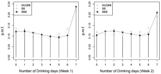
Figure 4.
Frequency distributions of the number of drinking days in weeks 1 and 2 and p.m.f.s for the BB, McGBB, and BBB distributions provided with the ML estimates reported in Table 2.
4.2. Candidate Assessment Data
In this section, we consider a dataset on candidate performance on an exam consisting of 9 questions. Each question is scored out of a total of 20 points, and when assessing a candidate’s final score, special attention is paid to the total number of questions on which he or she has an “alpha” (“alpha”—scoring at least 15 points on the question). The number of alphas is a rough indication of the quality of the candidate’s exam performance. Therefore, the distribution of alphas across candidates is of interest. A total of 209 candidates attempted questions from this 9-question section, and 326 alphas were awarded in total. Thus, we consider (number of trials/questions), where the dichotomous variable on each trial is whether or not the candidate scored an alpha.
For these data, we test the hypothesis : the data has exactly one mode versus the alternative hypothesis : the data have more than one mode, obtaining an observed statistic equal to 0.031, with a p-value equal to 0.720. Consequently, with a significance level equal to 0.05, is not rejected; that is, the frequency distribution of the data exhibits unimodal behavior.
A previous study with these data can be found in Paul [26].
Table 3 reports the results obtained by fitting the number of alphas using the BB, McGBB, and BBB distributions. In the table, it can be seen that the BBB distribution presents the highest p-values in the chi-square goodness-of-fit test and the lowest AIC and BIC values, suggesting that the BBB distribution should be selected among the fitted distributions for modeling the number of alphas.

Table 3.
ML estimates, maximum log-likelihood value, AIC and BIC values, and observed statistic (), degrees of freedom (DF), and p-value obtained in the chi-square goodness-of-fit tests for the BB, McGBB, and BBB distributions fitted to the number of alphas.
Figure 5 shows the frequency distribution of the number of alphas and the fitted BB, McGBB, and BBB distributions. In the figure, it can be seen that the frequency distribution of the number of alphas presents a single frequency peak and that the mass values of the BBB distribution are the closest to the empirical frequency values.
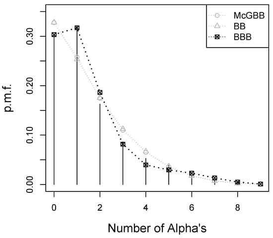
Figure 5.
Frequency distributions of the number of alphas and p.m.f.s for the BB, McGBB, and BBB distributions provided with the ML estimates reported in Table 3.
5. Final Comments
The beta-binomial (BB) and McDonald’s generalized beta-binomial (McGBB) distributions are discrete probability distributions used for modeling overdispersed binomial data. The McGBB distribution, presenting a larger parameter dimension than the BB distribution (three parameters), is capable of modeling even bimodality in cases where empirical frequency distributions present a bathtub shape. In this article, we propose the bimodal beta-binomial (BBB) distribution as an alternative for modeling overdispersed binomial data, both unimodal and bimodal. The new distribution arises from a weighted version of the BB distribution, where the weight function has the quadratic form proposed by Elal-Olivero [13]. Consequently, the BBB distribution is capable of presenting a flexible probability mass function in terms of shapes: monotonic, unimodal, and even bimodal. The bimodal shape of the BBB distribution is not limited to the bathtub shape (like the McGBB distribution), but the bimodality can be accompanied by various levels of skewness.
We derive the main structural functions of the BBB distribution, such as the p.m.f., the c.d.f., and the raw rth moment. We use the rth moment to describe the behavior of the coefficient of variation and the coefficient of skewness. We observe that the BBB distribution may exhibit a larger relative dispersion and a larger skewness than the BB distribution. We discuss parameter estimation via the maximum likelihood (ML) method. The estimators are not closed-form, so numerical methods are required to obtain the estimates. We develop a simulation study to evaluate the behavior of the ML estimators, in which we observe that the ML method provides acceptable estimates. Finally, we illustrate the utility of the BBB distribution by fitting real data sets. The illustrations show that the BBB distribution can outperform the BB and McGBB distributions in modeling count data that exhibit both unimodality and bimodality.
Author Contributions
Conceptualization, J.R., J.N.-Z. and D.-J.L.; Methodology, J.N.-Z., D.-J.L., J.A. and Y.A.I.; Software, J.A. and Y.A.I.; Validation, J.R., J.N.-Z., D.-J.L., J.A. and Y.A.I.; Formal analysis, J.R., J.N.-Z., D.-J.L., J.A. and Y.A.I.; Investigation, J.R., J.N.-Z., D.-J.L. and J.A.; Writing—review & editing, Y.A.I.; Supervision, J.R. All authors have read and agreed to the published version of the manuscript.
Funding
This research received no external funding.
Data Availability Statement
The original contributions presented in the study are included in the article, further inquiries can be directed to the corresponding author.
Conflicts of Interest
The authors declare no conflict of interest.
Appendix A. R Functions
The R codes used in this article are available at https://github.com/YuriIriarte/BBBdistribution (accessed on 18 September 2024) stored in the following files:
- BBB-distribution;Includes R codes for computing the structural functions of the BBB distribution.
| p.m.f. →dBBB(); c.d.f. → pBBB(); rth moment → momBBB() |
| coefficient of variation →coef.var(); skewness coefficient → skewnessBBB(). |
- 2.
- BB-McGBB-distribution;Includes R codes for computing the p.m.f.s of the BB and McGBB distributions.
| BB p.m.f. → dBB(); McGBB p.m.f. → dMcGBB(). |
- 3.
- Log-likelihood;Includes R codes for computing the log-likelihood functions to obtain the ML estimators using the optim() function.
| BB log-likelihood → loglikBB() |
| McGBB log-likelihood → loglikMcGBB() |
| BBB log-likelihood → loglikBBB(). |
- 4.
- Application-alcohol-week1 (week2);Includes the data and results obtained in the analysis in Section 4.1.
- 5.
- Application-candidate;Includes the data and results obtained in the analysis in Section 4.2.
References
- Böhning, D.; Dietz, E.; Schlattmann, P.; Mendonca, L.; Kirchner, U. The zero-inflated Poisson model and the decayed, missing and filled teeth index in dental epidemiology. J. R. Stat. Soc. Ser. A Stat. Soc. 1999, 162, 195–209. [Google Scholar] [CrossRef]
- Salman, A.K.; Fuchs, M.; Zampatti, D. Assessing risk factors of business failure in manufactoring sector: A count data approach from Sweden. Int. J. Econ. Commer. Manag. 2015, 3, 42–62. [Google Scholar]
- Calabria, R.; Guida, M.; Pulcini, G. Reliability analysis of repairable systems from in–service failure count data. Appl. Stoch. Model. Data Anal. 1994, 10, 141–151. [Google Scholar] [CrossRef]
- Alanko, T.; Lemmens, P.H. Response effects in consumption surveys: An application of the beta-binomial model to self-reported drinking frequencies. J. Off. Stat. 1996, 12, 253. [Google Scholar]
- Wilcox, R.R. A review of the beta-binomial model and its extensions. J. Educ. Stat. 1981, 6, 3–32. [Google Scholar] [CrossRef]
- Crowder, M.J. Beta-binomial ANOVA for proportions. Appl. Stat. 1978, 27, 34–37. [Google Scholar] [CrossRef]
- Tripathi, R.C.; Gupta, R.C.; Gurland, J. Estimation of parameters in the beta binomial model. Ann. Inst. Stat. Math. 1994, 46, 317–331. [Google Scholar] [CrossRef]
- Palm, B.G.; Bayer, F.M.; Cintra, R.J. Signal detection and inference based on the beta binomial autoregressive moving average model. Digit. Signal Process. 2021, 109, 102911. [Google Scholar] [CrossRef]
- Chen, H.; Li, Q.; Zhu, F. A covariate-driven beta-binomial integer-valued GARCH model for bounded counts with an application. Metrika 2023, 86, 805–826. [Google Scholar] [CrossRef]
- Jansen, K.; Holling, H. Rare events meta-analysis using the Bayesian beta-binomial model. Res. Synth. Methods 2023, 14, 853–873. [Google Scholar] [CrossRef]
- Fisher, R.A. The effect of methods of ascertainment upon the estimation of frequencies. Ann. Eugen. 1934, 6, 13–25. [Google Scholar] [CrossRef]
- Rao, C.R. On discrete distributions arising out of methods of ascertainment. Sankhyā Indian J. Stat. Ser. A 1965, 27, 311–324. [Google Scholar]
- Elal-Olivero, D. Alpha-skew-normal distribution. Proyecciones 2010, 29, 224–240. [Google Scholar] [CrossRef]
- Gómez-Déniz, E.; Pérez-Rodríguez, J.V.; Reyes, J.; Gómez, H.W. A bimodal discrete shifted Poisson distribution. a case study of tourists’ length of stay. Symmetry 2020, 12, 442. [Google Scholar] [CrossRef]
- Cortés, I.; Reyes, J.; Iriarte, Y.A. A Weighted Skew-Logistic Distribution with Applications to Environmental Data. Mathematics 2024, 12, 1287. [Google Scholar] [CrossRef]
- R Core Team. R: A Language and Environment for Statistical Computing; R Foundation for Statistical Computing: Vienna, Austria, 2023. [Google Scholar]
- Byrd, R.H.; Lu, P.; Nocedal, J.; Zhu, C. A limited memory algorithm for bound constrained optimization. SIAM J. Sci. Comput. 1995, 16, 1190–1208. [Google Scholar] [CrossRef]
- Neumann, V. Various techniques used in connection with random digits. Natl. Bur. Stand. 1951, 12, 36–38. [Google Scholar]
- Manoj, C.; Wijekoon, P.; Yapa, R.D. The McDonald generalized beta-binomial distribution: A new binomial mixture distribution and simulation based comparison with its nested distributions in handling overdispersion. Int. J. Stat. Probab. 2013, 2, 24. [Google Scholar] [CrossRef]
- Akaike, H. A new look at the statistical model identification. IEEE Trans. Autom. Control 1974, 19, 716–723. [Google Scholar] [CrossRef]
- Schwarz, G. Estimating the dimension of a model. Ann. Stat. 1978, 6, 461–464. [Google Scholar] [CrossRef]
- Ameijeiras-Alonso, J.; Crujeiras, R.M.; Rodríguez-Casal, A. Mode testing, critical bandwidth and excess mass. Test 2019, 28, 900–919. [Google Scholar] [CrossRef]
- Ameijeiras-Alonso, J.; Crujeiras, R.M.; Rodriguez-Casal, A. Multimode: An R package for mode assessment. arXiv 2018, arXiv:1803.00472. [Google Scholar] [CrossRef]
- Xiaohu, L.; Yanyan, H.; Xueyan, Z. The Kumaraswamy binomial distribution. Chin. J. Appl. Probab. Stat. 2011, 27, 511–521. [Google Scholar]
- Rodríguez-Avi, J.; Conde-Sánchez, A.; Sáez-Castillo, A.; Olmo-Jiménez, M. A generalization of the beta–binomial distribution. J. R. Stat. Soc. Ser. C Appl. Stat. 2007, 56, 51–61. [Google Scholar] [CrossRef]
- Paul, S. A three-parameter generalization of the binomial distribution. Hist. Philos. Log. 1985, 14, 1497–1506. [Google Scholar] [CrossRef]
Disclaimer/Publisher’s Note: The statements, opinions and data contained in all publications are solely those of the individual author(s) and contributor(s) and not of MDPI and/or the editor(s). MDPI and/or the editor(s) disclaim responsibility for any injury to people or property resulting from any ideas, methods, instructions or products referred to in the content. |
© 2024 by the authors. Licensee MDPI, Basel, Switzerland. This article is an open access article distributed under the terms and conditions of the Creative Commons Attribution (CC BY) license (https://creativecommons.org/licenses/by/4.0/).