Application of Gradient Optimization Methods in Defining Neural Dynamics

Abstract

Applications of gradient method for nonlinear optimization in development of Gradient Neural Network (GNN) and Zhang Neural Network (ZNN) are investigated. Particularly, the solution of the matrix equation $AXB=D$ which changes over time is studied using the novel GNN model, termed as GGNN$(A,B,D)$. The GGNN model is developed applying GNN dynamics on the gradient of the error matrix used in the development of the GNN model. The convergence analysis shows that the neural state matrix of the GGNN$(A,B,D)$ design converges asymptotically to the solution of the matrix equation $AXB=D$, for any initial state matrix. It is also shown that the convergence result is the least square solution which is defined depending on the selected initial matrix. A hybridization of GGNN with analogous modification GZNN of the ZNN dynamics is considered. The Simulink implementation of presented GGNN models is carried out on the set of real matrices.

1. Introduction and Background

Recurrent neural networks (RNNs) are an important class of algorithms for computing matrix (generalized) inverses. These algorithms are used to find the solutions of matrix equations or to minimize certain nonlinear matrix functions. RNNs are divided into two subgroups: Gradient Neural Networks (GNNs) and Zhang Neural Networks (ZNNs). The GNN design is explicit and mostly applicable to time-invariant problems, which means that the coefficients of the equations that are addressed are constant matrices. ZNN models can be implicit and are able to solve time-varying problems, where the coefficients of the equations depend on the variable $t\in \mathbb{R},t>0,$ representing time [1,2,3].

The Moore–Penrose inverse of $A\in {\mathrm{R}}^{p\times n}$ is the unique matrix $A^{†}=X\in {\mathrm{R}}^{n\times p}$ which is the solution to the well-known Penrose equations [4,5]:

$$A=AXA,X=XAX,AX={\left(AX\right)}^{\mathrm{T}},XA={\left(XA\right)}^{\mathrm{T}},$$

where ${\left(\right)}^{\mathrm{T}}$ denotes the transpose matrix. The rank of a matrix A, i.e., the maximum number of linearly independent columns in A, is denoted by $\mathrm{rank}\left(A\right)$.

Applications of linear algebra tools and generalized inverses can be found in important areas such as the modeling of electrical circuits [6], the estimation of DNA sequences [7] and the balancing of chemical equations [8,9], as well as in other important research domains related to robotics [10] and statistics [11]. A number of iterative methods for solving matrix equations based on gradient values have been proposed [12,13,14,15].

In the following sections, we will focus on GNN and ZNN dynamical systems based on the gradient of the objective function and their implementation. The main goal of this research is the analysis of convergence and the study of analytic solutions.

Models with GNN neural designs for computing the inverse or the Moore–Penrose inverse and linear matrix equations were proposed in [16,17,18,19]. Further, various dynamical systems aimed at approximating the pseudo-inverse of rank-deficient matrices were developed in [16]. Wei, in [20], proposed three RNN models for the approximation of the weighted Moore–Penrose inverse. Online matrix inversion in a complex matrix case was considered in [21]. A novel GNN design based on nonlinear activation functions (AFs) was proposed and analyzed in [22,23] for solving the constant Lyapunov matrix equation online. A fast convergent GNN aimed at solving a system of linear equations was proposed and numerically analyzed in [24]. Xiao, in [25], investigated the finite-time convergence of an appropriately accelerated ZNN for the online solution of the time-varying complex matrix equation $A\left(t\right)X\left(t\right)=B\left(t\right)$. A comparison with the corresponding GNN design was considered. Two improved nonlinear GNN dynamical systems for approximating the Moore–Penrose inverse of full-row or full-column rank matrices were proposed and considered in [26]. GNN-type models for solving matrix equations and computing related generalized inverses were developed in [1,3,13,16,18,20,27,28,29]. The acceleration of GNN dynamics to a finite-time convergence has been investigated recently. A finite-time convergent GNN for approximating online solutions of the general linear matrix equation $AX\left(t\right)B+CX\left(t\right)D=B$ was proposed in [30]. This goal was achieved using two activation functions (AFs) in the construction of the GNN. The influence of AFs on the convergence performance of a GNN design for solving the matrix equation $AXB+X=C$ was investigated in [31]. A fixed-time convergent GNN for solving the Sylvester equation was investigated in [32]. Moreover, noise-tolerant GNN models equipped with a suitable activation function (AF) able to solve convex optimization problems were developed in [33].

Our goal is to solve the equation $AXB=D$ and apply its particular cases in computing generalized inverses in real time by improving the GNN model developed in [34]. The developed dynamical system is denoted by GNN$(A,B,D)$. Or motivation is to improve the GNN model denoted by GNN$(A,B,D)$ and develop a novel gradient-based GGNN model, termed GGNN$(A,B,D)$, utilizing a novel type of dynamical system. The proposed GGNN model is based on the standard GNN dynamics along the gradient of the standard error matrix. The convergence analysis reveals the global asymptotic convergence of GGNN$(A,B,D)$ without restrictions, while the output belongs to the set of general solutions to the matrix equation $AXB=D$.

In addition, we propose gradient-based modifications of the hybrid models developed in [35] as proper combinations of GNN and ZNN models for solving the matrix equations $BX=D$ and $XC=D$ with constant coefficients. Analogous hybridizations for approximating the matrix inverse were developed in [36], while two modifications of the ZNN design for computing the Moore–Penrose inverse were proposed in [37]. Hybrid continuous-gradient–Zhang neural dynamics for solving linear time-variant equations were investigated in [38,39]. The developed hybrid GNN-ZNN models in this paper are aimed at solving the matrix equations $AX=B$ and $XC=D$, denoted by $\mathrm{HGZNN}(A,I,B)$ and $\mathrm{HGZNN}(I,C,D)$, respectively.

The implementation was performed in MATLAB Simulink, and numerical experiments were performed with simulations of the GNN, GGNN and HGZNN models.

The GNN used to solve the general linear matrix equation $AXB=D$ is defined over the error matrix $E\left(t\right)=D-AV\left(t\right)B$, where $t\in [0,+\infty )$ is time, and $V\left(t\right)$ is an unknown state-variable matrix that approximates the unknown matrix X in $AXB=D$. The goal function is $\epsilon \left(t\right)=\left|\right|D-{AV\left(t\right)B\left|\right|}_F^2/2$, where ${\parallel ·\parallel }_F=\sqrt{{\displaystyle \sum _{ij}}{a}_{ij}^2}$ denotes the Frobenius norm of a matrix. The gradient of $\epsilon \left(t\right)$ is equal to

$$\frac{\partial \epsilon \left(t\right)}{\partial V}=\nabla \epsilon =\frac{1}{2}\frac{\partial \left|\right|D-{AV\left(t\right)B\left|\right|}_F^2}{\partial V}=-A^{\mathrm{T}}(D-AV\left(t\right)B)B^{\mathrm{T}}.$$

The GNN evolutionary design is defined by the dynamic system

$$\dot{V}\left(t\right)=\frac{\mathrm{d}V\left(t\right)}{\mathrm{d}t}=-\gamma \frac{\partial \epsilon \left(t\right)}{\partial V},V\left(0\right)=V_0,$$

(1)

where $\gamma >0$ is a real parameter used to speed up the convergence, and $\dot{V}\left(t\right)$ denotes the time derivative of $V\left(t\right)$. Thus, the linear GNN aimed at solving $AXB=D$ is given by the following dynamics:

$$\dot{V}\left(t\right)=\gamma A^{\mathrm{T}}(D-AV\left(t\right)B)B^{\mathrm{T}}.$$

(2)

The dynamical flow (2) is denoted as GNN$(A,B,D)$. The nonlinear GNN$(A,B,D)$ for solving $AXB=D$ is defined by

$$\dot{V}\left(t\right)=\gamma A^{\mathrm{T}}\mathcal{F}(D-AV\left(t\right)B)B^{\mathrm{T}}.$$

(3)

The function array $\mathcal{F}\left(C\right)=\mathcal{F}\left(\left[c_{ij}\right]\right)$ is based on the appropriate odd and monotonically increasing activation function, which is applicable to the elements of a real matrix $C=\left(c_{ij}\right)\in {\mathbb{R}}^{m\times n}$, i.e., $\mathcal{F}\left(C\right)=\left[f\left(c_{ij}\right)\right],i=1,\dots ,m,j=1,\dots ,n,$.

Proposition 1 restates restrictions on the solvability of $AXB=D$ and its general solution.

Proposition 1

([4,5]). If $A\in {\mathbb{R}}^{m\times n},B\in {\mathbb{R}}^{p\times q}$ and $D\in {\mathbb{R}}^{m\times q}$, then the fulfillment of the condition

$$A{A}^{†}D{B}^{†}B=D$$

(4)

is necessary and sufficient for the solvability of the linear matrix equation $AXB=D$. In this case, the set of all solutions is given by

$$X=\left\{A^{†}D{B}^{†}+Y-A^{†}AYB{B}^{†}|Y\in {\mathbb{R}}^{n\times p}\right\}.$$

(5)

The following results from [34] describe the conditions of convergence and the limit of the unknown matrix $V\left(t\right)$ from (3) as $t\to +\infty$.

Proposition 2

([34]). Suppose the matrices $A\in {\mathbb{R}}^{m\times n},B\in {\mathbb{R}}^{p\times q}$ and $D\in {\mathbb{R}}^{m\times q}$ satisfy (4). Then, the unknown matrix $V\left(t\right)$ from (3) converges as $t\to +\infty$ with the equilibrium state

$$V\left(t\right)\to \tilde{V}=A^{†}D{B}^{†}+V\left(0\right)-A^{†}AV\left(0\right)B{B}^{†}$$

(6)

for any initial state-variable matrix $V\left(0\right)\in {\mathbb{R}}^{n\times p}.$

The research in [40] investigated various ZNN models based on optimization methods. The goal of the current research is to develop a GNN model based on the gradient $E_G\left(t\right)$ of ${\parallel E\left(t\right)\parallel }_F^2$ instead of the original goal function $E\left(t\right)$.

The obtained results are summarized as follows:

• A novel error function $E_G\left(t\right)$ is proposed for the development of the GNN dynamical evolution.
• The GNN design based on the error function $E_G\left(t\right)$ is developed and analyzed theoretically and numerically.
• A hybridization of GNN and ZNN dynamical systems based on the error matrix $E_G$ is proposed and investigated.

The overall organization of this paper is as follows. The motivation and derivation of the GGNN and GZNN models are presented in Section 2. Section 3 is dedicated to the convergence analysis of GGNN dynamics. A numerical comparison of GNN and GGNN dynamics is given in Section 4. Neural dynamics based on the hybridization of GGNN and GZNN models for solving matrix equations are considered in Section 6. Numerical examples of hybrid models are analyzed in Section 6. Finally, the last section presents some concluding remarks and a vision of further research.

2. Motivation and Derivation of GGNN and GZNN Models

The standard GNN design (2) solves the GLME $AXB=D$ under constraint (4). Our goal is to resolve this restriction and propose dynamic evolutions based on error functions that tend to zero without restrictions.

Our goal is to define the GNN design for solving the GLME $AXB=D$ based on the error function

$$E_G\left(t\right):=\nabla \epsilon \left(t\right)=A^{\mathrm{T}}\left(D-AV\left(t\right)B\right)B^{\mathrm{T}}=A^{\mathrm{T}}E\left(t\right)B^{\mathrm{T}}.$$

(7)

According to known results from nonlinear unconstrained optimization [41], the equilibrium points of (7) satisfy

$$E_G\left(t\right):=\nabla \epsilon \left(t\right)=0.$$

We continue the investigation from [40]. More precisely, we develop the GNN model based on the error function $E_G\left(t\right)$ instead of the error function $E\left(t\right)$. In this way, new neural dynamics are aimed at forcing the gradient $E_G$ to zero instead of the standard goal function $E\left(t\right)$. It is reasonable to call such an RNN model a gradient-based GNN (abbreviated GGNN).

Proposition 3 gives the conditions for the solvability of the matrix equations $E\left(t\right)=0$ and $E_G\left(t\right)=0$ and the general solutions to these systems.

Proposition 3

([40]). Consider the arbitrary matrices $A\in {\mathbb{R}}^{m\times n}$, $B\in {\mathbb{R}}^{k\times h}$ and $D\in {\mathbb{R}}^{m\times h}$. The following statements are true:

(a)

The equation $E\left(t\right)=0$ is solvable if and only if (4) is satisfied, and the general solution to $E\left(t\right)=0$ is given by (5).

(b)

The equation $E_G\left(t\right)=0$ is always solvable, and its general solution coincides with (5).

Proof. 

(a) This part of the proof follows from known results on the solvability and general solution of the matrix equation $AXB=D$ of generalized inverses [4] (p. 52, Theorem 1) and its application to the matrix equation $E\left(t\right)=0⟺AV\left(t\right)B=D$.

(b) According to [4] (p. 52, Theorem 1), the matrix equation

$$E_G\left(t\right)=0⟺A^{\mathrm{T}}AVB{B}^{\mathrm{T}}=A^{\mathrm{T}}D{B}^{\mathrm{T}}$$

is consistent if and only if

$$A^{\mathrm{T}}A{\left(A^{\mathrm{T}}A\right)}^{†}{A}^{\mathrm{T}}D{B}^{\mathrm{T}}{\left(B{B}^{\mathrm{T}}\right)}^{†}B{B}^{\mathrm{T}}=A^{\mathrm{T}}D{B}^{\mathrm{T}}$$

is satisfied. Indeed, applying the properties ${\left(A^{\mathrm{T}}A\right)}^{†}{A}^{\mathrm{T}}=A^{†}$, $B^T{\left(B{B}^{\mathrm{T}}\right)}^{†}=B^{†}$ and $A^{\mathrm{T}}A{A}^{†}=A^{\mathrm{T}}$, $B^{†}B{B}^{\mathrm{T}}=B^{\mathrm{T}}$ of the Moore–Penrose inverse [5] results in

$$A^{\mathrm{T}}A{\left(A^{\mathrm{T}}A\right)}^{†}{A}^{\mathrm{T}}D{B}^{\mathrm{T}}{\left(B{B}^{\mathrm{T}}\right)}^{†}B{B}^{\mathrm{T}}=A^{\mathrm{T}}A{A}^{†}D{B}^{†}B{B}^{\mathrm{T}}=A^{\mathrm{T}}D{B}^{\mathrm{T}}.$$

In addition, based on [4] (p. 52, Theorem 1), the general solution $V\left(t\right)$ to $E_G\left(t\right)=0$ is

$$\begin{array}{ll}V=& {\left(A^{\mathrm{T}}A\right)}^{†}{A}^{\mathrm{T}}D{B}^{\mathrm{T}}{\left(B{B}^{\mathrm{T}}\right)}^{†}+Y-{\left(A^{\mathrm{T}}A\right)}^{†}{A}^{\mathrm{T}}AYB{B}^{\mathrm{T}}{\left(B{B}^{\mathrm{T}}\right)}^{†}\\ & =A^{†}D{B}^{†}+Y-A^{†}AYB{B}^{†},\end{array}$$

(8)

which coincides with (5).    □

In this way, the matrix equation $E\left(t\right)=0$ is solvable under condition (4), while the equation $E_G\left(t\right)=0$ is always consistent. In addition, the general solutions to equations $E\left(t\right)=0$ and $E_G\left(t\right)=0$ are identical [40].

The next step is to define the GGNN dynamics using the error matrix $E_G\left(t\right)$. Let us define the objective function ${\epsilon }_G=\left|\right|E_G{\left|\right|}_F^2/2$, whose gradient is equal to

$$\frac{\partial {\epsilon }_G\left(V\left(t\right)\right)}{\partial V}=\frac{\partial \left|\right|A^{\mathrm{T}}(D-AV\left(t\right)B)B^{\mathrm{T}}{\left|\right|}_F^2}{\partial V}=-A^{\mathrm{T}}A\left(A^{\mathrm{T}}(D-AV\left(t\right)B)B^{\mathrm{T}}\right)B{B}^{\mathrm{T}}.$$

The dynamical system for the GGNN formula is obtained by applying the GNN evolution along the gradient of ${\epsilon }_G\left(V\left(t\right)\right)$ based on $E_G\left(t\right)$, as follows:

$$\begin{array}{cc}\hfill \dot{V}\left(t\right)& =-\gamma \frac{\partial {\epsilon }_G}{\partial V}\hfill \\ \hfill & =\gamma A^{\mathrm{T}}A\left(A^{\mathrm{T}}\left(D-AV\left(t\right)B\right)B^{\mathrm{T}}\right)B{B}^{\mathrm{T}}.\hfill \end{array}$$

(9)

The nonlinear GGNN dynamics are defined as

$$\dot{V}\left(t\right)=\gamma A^{\mathrm{T}}A\mathcal{F}\left(A^{\mathrm{T}}\left(D-AV\left(t\right)B\right)B^T\right)B{B}^{\mathrm{T}},$$

(10)

in which $\mathcal{F}\left(C\right)=\mathcal{F}\left(\left[c_{ij}\right]\right)$ denotes the elementwise application of an odd and monotonically increasing function $f(·)$, as  mentioned in the previous section for the GNN model (3). Model (10) is termed GGNN$(A,B,D)$. Three activation functions $f(·)$ are used in numerical experiments:

1.

Linear function

$$f_{lin}\left(x\right)=x;$$

(11)

2.

Power-sigmoid activation function

$$f_{ps}(x,\rho ,\varrho )=\left\{\begin{array}{ccc}\hfill x^{\rho }& \mathrm{if}& \left|x\right|\ge 1\hfill \\ \hfill \frac{1+e^{-\varrho }}{1-e^{-\varrho }}·\frac{1+e^{-\varrho x}}{1-e^{-\varrho x}}& \mathrm{if}& \left|x\right|<1\hfill \end{array}\right.$$

(12)

where $\varrho >2$, and $\rho \ge 3$ is an odd integer;

3.

Smooth power-sigmoid function

$$f_{sps}(x,\rho ,\varrho )=\frac{1}{2}{x}^{\rho }+\frac{1+e^{-\varrho }}{1-e^{-\varrho }}·\frac{1+e^{-\varrho x}}{1-e^{-\varrho x}},$$

(13)

where $\varrho >2$, and $\rho \ge 3$ is an odd integer.

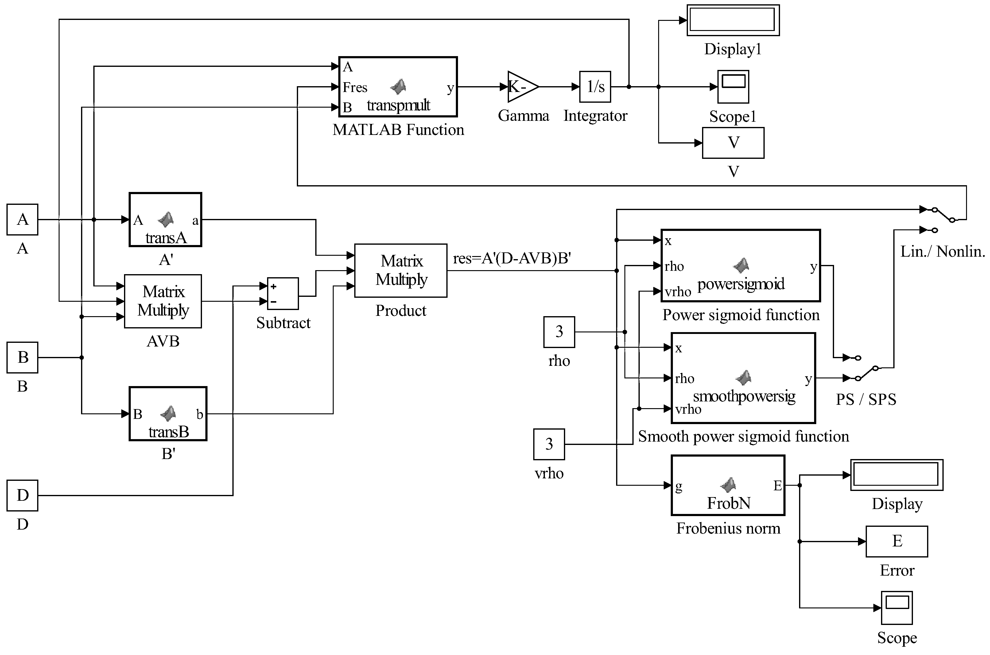
Figure 1 represents the Simulink implementation of GGNN$(A,B,D)$ dynamics (10).

On the other hand, the GZNN model, defined using the ZNN dynamics on the Zhangian matrix $E_G\left(t\right)$, is defined in [40] by the general evolutionary design

$${\dot{E}}_G\left(t\right)=\frac{\mathrm{d}{E}_G\left(t\right)}{\mathrm{d}t}=-\gamma \mathcal{F}\left(E_G\left(t\right)\right).$$

(14)

3. Convergence Analysis of GGNN Dynamics

In this section, we will analyze the convergence properties of the GGNN model given by dynamics (10).

Theorem 1.

Consider matrices $A\in {\mathbb{R}}^{m\times n},B\in {\mathbb{R}}^{p\times q}$ and $D\in {\mathbb{R}}^{m\times q}$. If an odd and monotonically increasing array activation function $\mathcal{F}(·)$ based on an elementwise function $f(·)$ is used, then the activation state matrix $V\left(t\right)\in {\mathbb{R}}^{n\times p}$ of the $\mathrm{GGNN}(A,B,D)$ model (10) asymptotically converges to the solution of the matrix equation $AXB=D$, i.e., $A^{\mathrm{T}}AV\left(t\right)B{B}^{\mathrm{T}}\to A^{\mathrm{T}}D{B}^{\mathrm{T}}$ as $t\to +\infty$, for an arbitrary initial state matrix $V\left(0\right)$.

Proof. 

From statement (b) of Proposition 3, the solvability of $A^{\mathrm{T}}AVB{B}^{\mathrm{T}}=A^{\mathrm{T}}D{B}^{\mathrm{T}}$ is ensured. The substitution $V\left(t\right)=\overline{V}\left(t\right)+A^{†}D{B}^{†}$ transforms the dynamics (10) into

$$\begin{array}{cc}\hfill \frac{\mathrm{d}\overline{V}\left(t\right)}{\mathrm{d}t}& =\frac{\mathrm{d}V\left(t\right)}{\mathrm{d}t}=\gamma A^{\mathrm{T}}A\mathcal{F}\left(A^{\mathrm{T}}\left(D-AV\left(t\right)B\right)B^{\mathrm{T}}\right)B{B}^{\mathrm{T}}\hfill \\ \hfill & =\gamma A^{\mathrm{T}}A\mathcal{F}\left(A^{\mathrm{T}}\left(D-A\overline{V}\left(t\right)B-A{A}^{†}D{B}^{†}B\right)B^{\mathrm{T}}\right)B{B}^{\mathrm{T}}\hfill \\ \hfill & \stackrel{\left(4\right)}{=}\gamma A^{\mathrm{T}}A\mathcal{F}\left(A^{\mathrm{T}}\left(D-A\overline{V}\left(t\right)B-D\right)B^{\mathrm{T}}\right)B{B}^{\mathrm{T}}\hfill \\ \hfill & =-\gamma A^{\mathrm{T}}A\mathcal{F}\left(A^{\mathrm{T}}A\overline{V}\left(t\right)B{B}^{\mathrm{T}}\right)B{B}^{\mathrm{T}}.\hfill \end{array}$$

(15)

The Lyapunov function candidate that measures the convergence performance is defined by

$$L\left(\overline{V}\left(t\right),t\right)=\frac{1}{2}\left|\right|\overline{V}\left(t\right){\left|\right|}_F^2=\frac{1}{2}\mathrm{Tr}\left(\overline{V}{\left(t\right)}^{\mathrm{T}}\overline{V}\left(t\right)\right).$$

(16)

The conclusion is $L(\overline{V}\left(t\right),t)\ge 0$. According to (16), assuming (15) and using $\mathrm{d}\mathrm{Tr}\left(X^{\mathrm{T}}X\right)=2\mathrm{Tr}\left(X^{\mathrm{T}}\mathrm{d}X\right)$, in conjunction with the basic properties of the matrix trace function, one can express the time derivative of $L(\overline{V}\left(t\right),t)$ as follows:

$$\begin{array}{cc}\hfill \frac{\mathrm{d}L(\overline{V}\left(t\right),t)}{\mathrm{d}t}& =\frac{1}{2}\frac{\mathrm{d}\mathrm{Tr}\left(\overline{V}{\left(t\right)}^{\mathrm{T}}\overline{V}\left(t\right)\right)}{\mathrm{d}t}\hfill \\ \hfill & =\frac{1}{2}·2·\mathrm{Tr}\left(\overline{V}{\left(t\right)}^{\mathrm{T}}\frac{\mathrm{d}\overline{V}\left(t\right)}{\mathrm{d}t}\right)\hfill \\ \hfill & =\mathrm{Tr}\left[\overline{V}{\left(t\right)}^{\mathrm{T}}\left(-\gamma A^{\mathrm{T}}A\mathcal{F}\left(A^{\mathrm{T}}A\overline{V}\left(t\right)B{B}^{\mathrm{T}}\right)B{B}^{\mathrm{T}}\right)\right]\hfill \\ \hfill & =-\gamma \mathrm{Tr}\left[\overline{V}{\left(t\right)}^{\mathrm{T}}{A}^{\mathrm{T}}A\mathcal{F}\left(A^{\mathrm{T}}A\overline{V}\left(t\right)B{B}^{\mathrm{T}}\right)B{B}^{\mathrm{T}}\right]\hfill \\ \hfill & =-\gamma \mathrm{Tr}\left[B{B}^{\mathrm{T}}\overline{V}{\left(t\right)}^{\mathrm{T}}{A}^{\mathrm{T}}A\mathcal{F}\left(A^{\mathrm{T}}A\overline{V}\left(t\right)B{B}^{\mathrm{T}}\right)\right]\hfill \\ \hfill & =-\gamma \mathrm{Tr}\left[{\left(A^{\mathrm{T}}A\overline{V}\left(t\right)B{B}^{\mathrm{T}}\right)}^{\mathrm{T}}\mathcal{F}\left(A^{\mathrm{T}}A\overline{V}\left(t\right)B{B}^{\mathrm{T}}\right)\right].\hfill \end{array}$$

(17)

Since the scalar-valued function $f(·)$ is odd and monotonically increasing, it follows that, for $W\left(t\right)=A^{\mathrm{T}}A\overline{V}\left(t\right)B{B}^{\mathrm{T}},$

$$\begin{array}{cc}\hfill \frac{\mathrm{d}L(\overline{V}\left(t\right),t)}{\mathrm{d}t}& =-\gamma \mathrm{Tr}\left[\left(W^{\mathrm{T}}\mathcal{F}\left(W\right)\right)\right]\hfill \\ \hfill & =-\gamma \sum _{i=1}^m\sum _{j=1}^n{w}_{ij}f\left(w_{ij}\right)\left\{\begin{array}{ccc}\hfill <0& \mathrm{if}& W\left(t\right):=A^{\mathrm{T}}A\overline{V}\left(t\right)B{B}^{\mathrm{T}}\ne 0\hfill \\ \hfill =0& \mathrm{if}& W\left(t\right):=A^{\mathrm{T}}A\overline{V}\left(t\right)B{B}^{\mathrm{T}}=0,\hfill \end{array}\right.\hfill \end{array}$$

(18)

which implies

$$\frac{\mathrm{d}L(\overline{V}\left(t\right),t)}{\mathrm{d}t}\left\{\begin{array}{ccc}\hfill <0& \mathrm{if}& W\left(t\right)\ne 0\hfill \\ \hfill =0& \mathrm{if}& W\left(t\right)=0.\hfill \end{array}\right.$$

(19)

Observing the identity

$$\begin{array}{cc}\hfill W\left(t\right)& =A^{\mathrm{T}}A\overline{V}\left(t\right)B{B}^{\mathrm{T}}\hfill \\ \hfill & =A^{\mathrm{T}}A\left(V\left(t\right)-A^{†}D{B}^{†}\right)B{B}^{\mathrm{T}}\hfill \\ \hfill & =A^{\mathrm{T}}AV\left(t\right)B{B}^{\mathrm{T}}-A^{\mathrm{T}}D{B}^{\mathrm{T}}\hfill \\ \hfill & =A^{\mathrm{T}}\left(AV\left(t\right)B-D\right)B^{\mathrm{T}},\hfill \end{array}$$

and using the Lyapunov stability theory, $W\left(t\right):=A^{\mathrm{T}}\left(AV\left(t\right)B-D\right)B^{\mathrm{T}}$ globally converges to the zero matrix from an arbitrary initial value $V\left(0\right)$.    □

Theorem 2.

The activation state-variable matrix $V\left(t\right)$ of the model $\mathrm{GGNN}(A,B,D)$, defined by (10), is convergent as $t\to +\infty$, and its equilibrium state is

$$V\left(t\right)\to \tilde{V}\left(t\right)=A^{†}D{B}^{†}+V\left(0\right)-A^{†}AV\left(0\right)B{B}^{†}$$

(20)

for every initial state matrix $V\left(0\right)\in {\mathbb{R}}^{n\times p}$.

Proof. 

From (10), the matrix $V_1\left(t\right)={\left(A^{\mathrm{T}}A\right)}^{†}{A}^{\mathrm{T}}AV\left(t\right)B{B}^{\mathrm{T}}{\left(B{B}^{\mathrm{T}}\right)}^{†}$ satisfies

$$\begin{array}{cc}\hfill \frac{\mathrm{d}{V}_1\left(t\right)}{\mathrm{d}t}& ={\left(A^{\mathrm{T}}A\right)}^{†}{A}^{\mathrm{T}}A\frac{\mathrm{d}V\left(t\right)}{\mathrm{d}t}B{B}^{\mathrm{T}}{\left(B{B}^{\mathrm{T}}\right)}^{†}\hfill \\ \hfill & =\gamma {\left(A^{\mathrm{T}}A\right)}^{†}{A}^{\mathrm{T}}A\left[A^{\mathrm{T}}A\left(A^{\mathrm{T}}(D-AV\left(t\right)B)B^{\mathrm{T}}\right)B{B}^{\mathrm{T}}\right]B{B}^{\mathrm{T}}{\left(B{B}^{\mathrm{T}}\right)}^{†}.\hfill \end{array}$$

According to the basic properties of the Moore–Penrose inverse [5], it follows that

$${\left(B{B}^{\mathrm{T}}\right)}^{\mathrm{T}}B{B}^{\mathrm{T}}{\left(B{B}^{\mathrm{T}}\right)}^{†}={\left(B{B}^{\mathrm{T}}\right)}^{\mathrm{T}}=B{B}^{\mathrm{T}},{\left(A^{\mathrm{T}}A\right)}^{†}{A}^{\mathrm{T}}A{\left(A^{\mathrm{T}}A\right)}^{\mathrm{T}}={\left(A^{\mathrm{T}}A\right)}^{\mathrm{T}}=A^{\mathrm{T}}A$$

which further implies

$$\begin{array}{cc}\hfill \frac{\mathrm{d}{V}_1\left(t\right)}{\mathrm{d}t}& =\gamma A^{\mathrm{T}}A\left(A^{\mathrm{T}}(D-AV\left(t\right)B)B^{\mathrm{T}}\right)B{B}^{\mathrm{T}}\hfill \\ & =\frac{\mathrm{d}V\left(t\right)}{\mathrm{d}t}.\hfill \end{array}$$

Consequently, $V_2\left(t\right)=V\left(t\right)-V_1\left(t\right)$ satisfies $\frac{\mathrm{d}{V}_2\left(t\right)}{\mathrm{d}t}=\frac{\mathrm{d}V\left(t\right)}{\mathrm{d}t}-\frac{\mathrm{d}{V}_1\left(t\right)}{\mathrm{d}t}=0$, which implies

$$\begin{array}{cc}\hfill V_2\left(t\right)& =V_2\left(0\right)\hfill \\ \hfill & =V\left(0\right)-V_1\left(0\right)\hfill \\ \hfill & =V\left(0\right)-{\left(A^{T}A\right)}^{†}{A}^{\mathrm{T}}AV\left(0\right)B{B}^{\mathrm{T}}{\left(B{B}^{\mathrm{T}}\right)}^{†}\hfill \\ \hfill & =V\left(0\right)-A^{†}AV\left(0\right)B{B}^{†},t\ge 0.\hfill \end{array}$$

(21)

Furthermore, from Theorem 1, $A^{\mathrm{T}}AV\left(t\right)B{B}^{\mathrm{T}}\to A^{\mathrm{T}}D{B}^{\mathrm{T}}$, and $V_1\left(t\right)$ converges to

$$\begin{array}{ll}{V}_1\left(t\right)& ={\left(A^{\mathrm{T}}A\right)}^{†}{A}^{\mathrm{T}}AV\left(t\right)B{B}^{\mathrm{T}}{\left(B{B}^{\mathrm{T}}\right)}^{†}\to {\left(A^{\mathrm{T}}A\right)}^{†}{A}^{\mathrm{T}}D{B}^{\mathrm{T}}{\left(B{B}^{\mathrm{T}}\right)}^{†}\\ & =A^{†}D{B}^{†}\end{array}$$

as $t\to +\infty$. Therefore, $V\left(t\right)=V_1\left(t\right)+V_2\left(t\right)$ converges to the equilibrium state

$$\tilde{V}\left(t\right)=A^{†}D{B}^{†}+V_2\left(t\right)=A^{†}D{B}^{†}+V\left(0\right)-A^{†}AV\left(0\right)B{B}^{†}.$$

The proof is finished.    □

4. Numerical Experiments on GNN and GGNN Dynamics

The numerical examples in this section are based on the Simulink implementation of the GGNN formula in Figure 1.

The parameter $\gamma$, initial state $V\left(0\right)$ and parameters $\rho$ and $\varrho$ of the nonlinear activation functions (12) and (13) are entered directly into the model, while matrices A, B and D are defined from the workspace. It is assumed that $\rho =\varrho =3$ in all examples. The ode15s differential equation solver is used in the configuration parameters. In all examples, $V^{*}$ denotes the theoretical solution.

The blocks powersig, smoothpowersig and transpmult include the codes described in [34,42].

Example 1.

Let us consider the idempotent matrix A from [43,44],

$$A=\left[\begin{array}{cccc}1& 0& 1& 1\\ 0& 1& 1& 2\\ 0& 0& 0& 0\\ 0& 0& 0& 0\end{array}\right]$$

of $\mathrm{rank}\left(A\right)=2$, and the theoretical Moore–Penrose inverse

$$V^{*}=A^{†}=\frac{1}{3}\left[\begin{array}{cccc}2& -1& 0& 0\\ -1& 1& 0& 0\\ 1& 0& 0& 0\\ 0& 1& 0& 0\end{array}\right].$$

The matrix equation corresponding to the Moore–Penrose inverse is $A^{\mathrm{T}}AX=A^{\mathrm{T}}$ [16], which implies the error function $E\left(t\right)=A^{\mathrm{T}}(I-AX)$. The corresponding GNN model is defined by GNN$(A^{\mathrm{T}}A,I_4,A^{\mathrm{T}})$, where $I_4$ denotes the identity and zero $4\times 4$ matrix. Constraint (4) reduces to the condition $A{A}^{†}{A}^{\mathrm{T}}=A^{\mathrm{T}}$, which is not satisfied. The input parameters of GNN$(A^{\mathrm{T}}A,I_4,A^{\mathrm{T}})$ are $\gamma ={10}^8$, $V\left(0\right)=O_4$, where $O_4$ denotes the zero $4\times 4$ matrix. The corresponding GGNN$({\left(A^{\mathrm{T}}A\right)}^2,$$I,A^{\mathrm{T}}A{A}^{\mathrm{T}})$ design is based on the error matrix $E_G\left(t\right)=A^{\mathrm{T}}A{A}^{\mathrm{T}}\left(I-AV\right).$ The Simulink implementation of GGNN$(A,B,D)$ from Figure 1 and the Simulink implementation of GNN$(A,B,D)$ from [34] export, in this case, the graphical results presented in Figure 2 and Figure 3, which display the behaviors of the norms $\left|\right|E_G{\left(t\right)\left|\right|}_F=\left|\right|A^{\mathrm{T}}A{A}^{\mathrm{T}}(I-AV\left(t\right)){\left|\right|}_F$ and $\left|\right|V\left(t\right)-V^{*}{\left|\right|}_F$, respectively. It is observable that the norms generated by the application of the GGNN formula vanish faster to zero than the corresponding norms in the GNN model. The graphs in the presented figures strengthen the fast convergence of the GGNN dynamical system and its important role, which can include the application of this specific model (10) to problems that require the computation of the Moore–Penrose inverse.

Example 2.

Let us consider the matrices

$$A=\left[\begin{array}{ccc}-8& 8& -4\\ 11& 4& -7\\ 1& -4& 3\\ 0& 12& -10\\ 6& 12& -12\end{array}\right],B=\left[\begin{array}{ccc}1& 0& 0\\ 0& 1& 0\\ 0& 0& 1\\ 0& 0& 0\end{array}\right],D=\left[\begin{array}{ccc}-84& 2524& 304\\ -2252& -623& 2897\\ 484& -885& -701\\ -1894& 2278& 2652\\ -2778& 1524& 3750\end{array}\right].$$

The exact minimum-norm least-squares solution is

$$V^{*}=A^{†}D{B}^{†}=\left[\begin{array}{cccc}-\frac{7409}{65}& -\frac{9564}{65}& \frac{8953}{65}& 0\\ -\frac{968}{13}& \frac{1770}{13}& \frac{1402}{13}& 0\\ \frac{6503}{65}& -\frac{4187}{65}& -\frac{8826}{65}& 0\end{array}\right].$$

The ranks of the input matrices are equal to $r=\mathrm{rank}\left(A\right)=2$, $\mathrm{rank}\left(D\right)=2$ and $\mathrm{rank}\left(B\right)=3$. Constraint (4) is satisfied in this case. The linear GGNN$(A,B,D)$ formula (10) is applied to solve the matrix equation $AXB=D$. The gain parameter of the model is $\gamma ={10}^9$, $V\left(0\right)=0$, and the stopping time is $t=0.00001$, which gives

$$X=\left[\begin{array}{cccc}-113.9846& -147.1385& 137.7385& 0\\ -74.4615& 136.1538& 107.8462& 0\\ 100.0462& -64.4154& -135.7846& 0\end{array}\right]\approx A^{†}D{B}^{†}.$$

The elementwise trajectories of the state variables $v_{ij}$ of the state matrix $V\left(t\right)$ are shown in Figure 4a–c with solid red lines for linear, power-sigmoid and smooth power-sigmoid activation functions, respectively. The fast convergence of elementwise trajectories to the corresponding black dashed trajectories of the theoretical solution $V^{*}$ is notable. In addition, faster convergence caused by the nonlinear AFs $f_{ps}$ and $f_{sps}$ is noticeable in Figure 4b,c. The trajectories in the figures indicate the usual convergence behavior, so the system is globally asymptotically stable. The norms of the error matrix $E_G$ of both models GNN and GGNN under linear and nonlinear AFs are shown in Figure 5a–c. The power-sigmoid and smooth power-sigmoid activation functions show superiority in their convergence speed compared with linear activation. On each graph in Figure 5a–c, the Frobenius norm $\parallel E_G{\left(t\right)\parallel }_F$ of the error matrix $E_G\left(t\right)$ in the GGNN formula vanishes faster to zero than that in the GNN model. Moreover, in each graph in Figure 6a–c, the Frobenius norm ${\parallel E\left(t\right)\parallel }_F$ in the GGNN formula vanishes faster to zero than that in the GNN model, which strengthens the fact that the proposed dynamical system (10) initiates accelerated convergence compared to (3).

All graphs shown in Figure 5 and Figure 6 confirm the applicability of the proposed GGNN design compared to the traditional GNN design, even if constraint (4) holds.

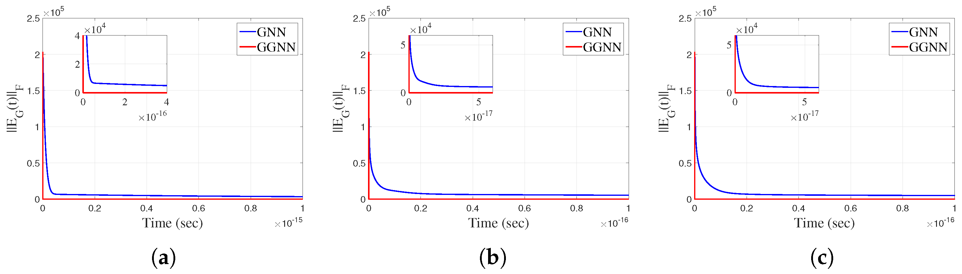
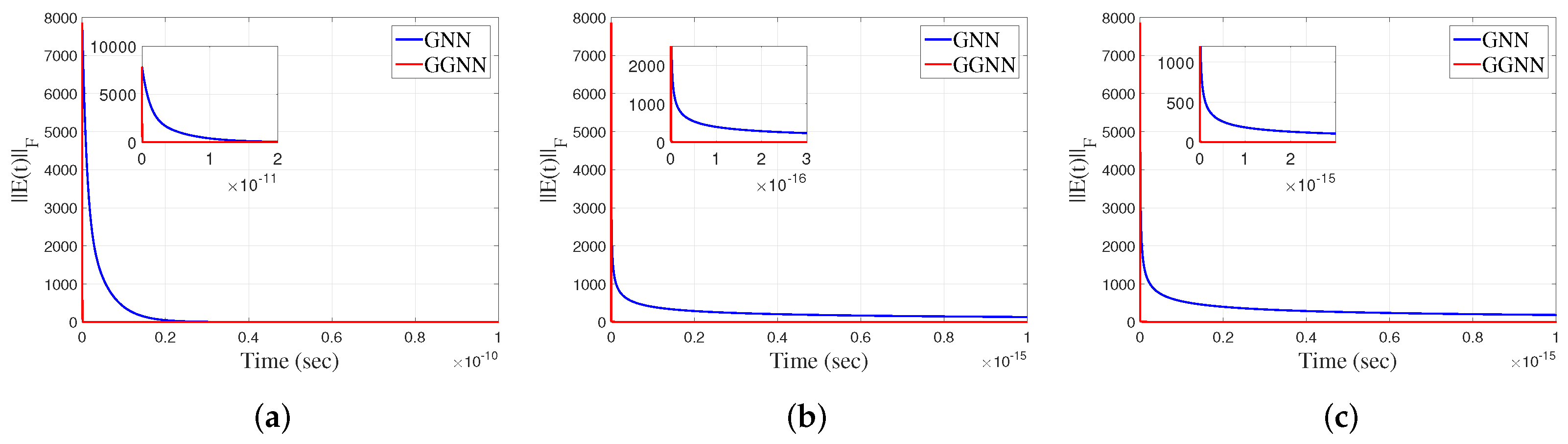
Example 3.

Let us explore the behavior of GNN and GGNN dynamics for computing the Moore–Penrose inverse of the matrix

$$A=\left[\begin{array}{ccc}9& 3& -3\\ -1& 1& 0\\ 4& 7& 2\\ 2& 4& -4\\ 13& 5& 8\end{array}\right].$$

The Moore–Penrose inverse of A is equal to

$$\begin{array}{ll}{A}^{†}& =\left[\begin{array}{ccccc}\frac{9908}{127779}& -\frac{18037}{766674}& -\frac{6874}{127779}& -\frac{2663}{383337}& \frac{29941}{766674}\\ -\frac{5690}{127779}& \frac{14426}{383337}& \frac{16741}{127779}& \frac{25130}{383337}& -\frac{6392}{383337}\\ -\frac{3517}{42593}& \frac{1979}{255558}& \frac{1073}{42593}& -\frac{7373}{127779}& \frac{15049}{255558}\end{array}\right]\\ & \approx \left[\begin{array}{ccccc}0.0775& -0.0235& -0.0538& -0.0069& 0.0390\\ -0.0445& 0.0376& 0.1310& 0.0655& -0.0167\\ -0.0826& 0.0077& 0.0252& -0.0577& 0.0589\end{array}\right].\end{array}$$

The rank of the input matrix is equal to $r=\mathrm{rank}\left(A\right)=3$. Consequently, the matrix A is left invertible and satisfies $A^{†}A=I$. The error matrix $E\left(t\right)=I-VA$ initiates the GNN$(I,A,I)$ dynamics for computing $A^{†}$. The gradient-based error matrix

$$E_G\left(t\right)=\left(I-V\left(t\right)A\right)A^{\mathrm{T}}.$$

initiates the GGNN$(I,A{A}^{\mathrm{T}},A^{\mathrm{T}})$ design.

The gain parameter of the model is $\gamma =100$, and the initial state is $V\left(0\right)=0$ with a stop time $t=0.00001$.

The Frobenius norms of the error matrix $E\left(t\right)$ generated by the linear GNN and GGNN models for different values of γ ($\gamma ={10}^2,\gamma ={10}^3,\gamma ={10}^6$) are shown in Figure 7a–c. The graphs in these figures confirm an increase in the convergence speed, which is caused by the increase in the gain parameter γ. Because of that, the considered time intervals are $[0,{10}^{-2}]$, $[0,{10}^{-3}]$ and $[0,{10}^{-6}]$, respectively. In all three scenarios, a faster convergence of the GGNN model is observable compared to the GNN design. The values of the norm $\parallel E_G{\parallel }_F$ generated by both the GNN and GGNN models with linear and two nonlinear activation functions are shown in Figure 8a–c. Like the conclusion in the previous example, the perception is that the GGNN converges faster compared to the GNN model.

In addition, the graphs in Figure 8b,c, corresponding to the power-sigmoid and smooth power-sigmoid AFs, respectively, show a certain level of instability in convergence, as well as an increase in the value of $\parallel E_G{\left(t\right)\parallel }_F$.

Example 4.

Consider the matrices

$$A=\left[\begin{array}{ccccc}15& -352& -45& -238& 42\\ -5& 14& 8& 132& -65\\ 235& -65& 44& 350& -73\end{array}\right],D=\left[\begin{array}{ccc}-4& 4& 16\\ 3& 1& -9\\ 1& -7& 2\\ 2& 2& -4\\ 4& 1& -5\end{array}\right],A_1=DA,$$

which dissatisfy $\mathrm{rank}\left(A_1\right)=\mathrm{rank}\left(D\right)=3$. Now, we apply the GNN and GGNN formulae to solve the matrix equation $A_{1}X=D$. The standard error function is defined as $E\left(t\right)=D-A_{1}V\left(t\right)$. So, we consider GNN$(A_1,I_3,D)$. The error matrix for the corresponding GGNN model is $E_G\left(t\right)=A_1^{\mathrm{T}}(D-A_{1}V\left(t\right)),$ which initiates the GGNN$(A_1^{\mathrm{T}}{A}_1,I_3,A_1^{\mathrm{T}}D)$ flow. The gain parameter of the model is $\gamma ={10}^9$, and the final time is $t=0.00001$. The zero initial state $V\left(0\right)=0$ generates the best approximate solution $X=A_1^{†}D={\left(DA\right)}^{†}D$ of the matrix equation $A_{1}X=D$, given by

$$\begin{array}{ll}X=A_1^{†}D& =\left[\begin{array}{ccc}-\frac{133851170015}{180355524917879}& -\frac{1648342203725}{180355524917879}& \frac{608888775010}{180355524917879}\\ -\frac{508349079720}{180355524917879}& -\frac{691967699675}{180355524917879}& -\frac{48398092277}{180355524917879}\\ -\frac{68130232042}{180355524917879}& -\frac{242513061343}{180355524917879}& \frac{82710890618}{180355524917879}\\ -\frac{31936168532}{180355524917879}& \frac{727110260384}{180355524917879}& \frac{134047117682}{180355524917879}\\ -\frac{172434574901}{180355524917879}& -\frac{1350198643304}{180355524917879}& \frac{225136761416}{180355524917879}\end{array}\right]\\ & \approx \left[\begin{array}{ccc}-0.000742& -0.00914& 0.00338\\ -0.00282& -0.00384& -0.000268\\ -0.000378& -0.00134& 0.000459\\ -0.000177& 0.00403& 0.000743\\ -0.000956& -0.00749& 0.00125\end{array}\right].\end{array}$$

The Frobenius norms of the error matrix $E\left(t\right)=D-A_{1}V\left(t\right)B$ in the GNN and GGNN models for both linear and nonlinear activation functions are shown in Figure 9a–c, and the error matrix $E_G\left(t\right)=A_1^{\mathrm{T}}(D-A_{1}V\left(t\right))$ in both models for linear and nonlinear activation functions are shown in Figure 10a–c. It is observable that the GGNN converges faster than GNN.

Example 5.

Table 1. Input data.

Matrix A			Matrix B			Matrix D			Input and Residual Norm
$\mathit{m}$	$\mathit{n}$	$\mathbf{rank}\left(\mathit{A}\right)$	$\mathit{p}$	$\mathit{q}$	$\mathbf{rank}\left(\mathit{B}\right)$	$\mathit{m}$	$\mathit{q}$	$\mathbf{rank}\left(\mathit{D}\right)$	$\mathit{\gamma }$	${\mathit{t}}_{\mathit{f}}$	$\parallel {\mathit{AA}}^{†}{\mathit{DB}}^{†}{\mathit{B}-\mathit{D}\parallel }_{\mathit{F}}$
10	8	8	9	7	7	10	7	7	${10}^4$	0.5	1.051
10	8	6	9	7	7	10	7	7	${10}^4$	0.5	1.318
10	8	6	9	7	5	10	7	7	${10}^4$	0.5	1.81
10	8	6	9	7	5	10	7	5	${10}^4$	5	2.048
10	8	1	9	7	2	10	7	1	${10}^4$	5	2.372
20	10	10	8	5	5	20	5	5	${10}^6$	5	1.984
20	10	5	8	5	5	20	5	5	${10}^6$	5	2.455
20	10	5	8	5	2	20	5	5	${10}^6$	1	3.769
20	10	2	8	5	2	20	5	2	${10}^6$	1	2.71
20	15	15	5	2	2	20	2	2	${10}^8$	1	1.1
20	15	10	5	2	2	20	2	2	${10}^8$	1	1.158
20	15	10	5	2	1	20	2	2	${10}^8$	1	2.211
20	15	5	5	2	1	20	2	2	${10}^8$	1	1.726

and

Table 2. Experimental results based on data presented in Table 1.

${\left|\right|\mathit{E}\left(\mathit{t}\right)\left|\right|}_{\mathit{F}}$ (GNN)	${\left|\right|\mathit{E}\left(\mathit{t}\right)\left|\right|}_{\mathit{F}}$ (GGNN)	$\left|\right|{\mathit{E}}_{\mathit{G}}\left(\mathit{t}\right){\left|\right|}_{\mathit{F}}$ (GNN)	$\left|\right|{\mathit{E}}_{\mathit{G}}\left(\mathit{t}\right){\left|\right|}_{\mathit{F}}$ (GGNN)	CPU (GNN)	CPU (GGNN)
$\mathbf{1}.\mathbf{051}$	$1.094$	$\mathbf{2}.\mathbf{52}\times {\mathbf{10}}^{-\mathbf{9}}$	$0.02524$	$\mathbf{5}.\mathbf{017148}$	$13.470995$
$\mathbf{1}.\mathbf{318}$	1.393	$\mathbf{3}.\mathbf{122}\times {\mathbf{10}}^{-\mathbf{7}}$	0.03661	22.753954	$\mathbf{10}.\mathbf{734163}$
$\mathbf{1}.\mathbf{811}$	1.899	$\mathbf{0}.\mathbf{0008711}$	0.03947	15.754537	$\mathbf{15}.\mathbf{547785}$
$\mathbf{2}.\mathbf{048}$	2.082	$\mathbf{1}.\mathbf{96}\times {\mathbf{10}}^{-\mathbf{10}}$	0.00964	$\mathbf{9}.\mathbf{435709}$	17.137916
$\mathbf{2}.\mathbf{372}$	$\mathbf{2}.\mathbf{372}$2	$\mathbf{1}.\mathbf{7422}\times {\mathbf{10}}^{-\mathbf{15}}$	2.003 $\times {10}^{-15}$	21.645386	$\mathbf{13}.\mathbf{255210}$
$\mathbf{1}.\mathbf{984}$	$\mathbf{1}.\mathbf{984}$	2.288 $\times {10}^{-14}$	9.978 $\times {\mathbf{10}}^{-\mathbf{15}}$	21.645386	13.255210
2.455	2.455	1.657 $\times {10}^{-11}$	1.693 $\times {\mathbf{10}}^{-\mathbf{14}}$	50.846893	19.059385
3.769	3.769	6.991 $\times {10}^{-11}$	4.071 $\times {\mathbf{10}}^{-\mathbf{14}}$	42.184748	13.722390
2.71	2.71	1.429 $\times {10}^{-14}$	1.176 $\times {\mathbf{10}}^{-\mathbf{14}}$	148.484258	13.527065
1.1	1.1	1.766 $\times {10}^{-13}$	5.949 $\times {\mathbf{10}}^{-\mathbf{15}}$	218.169376	17.5666568
1.158	1.158	2.747 $\times {10}^{-10}$	2.981 $\times {\mathbf{10}}^{-\mathbf{13}}$	45.505618	12.441782
2.211	2.211	7.942 $\times {10}^{-12}$	8.963 $\times {\mathbf{10}}^{-\mathbf{14}}$	194.605133	14.117241
1.726	1.726	8.042 $\times {10}^{-15}$	3.207 $\times {\mathbf{10}}^{-\mathbf{15}}$	22.340501	11.650829

show the results obtained during experiments we conducted with nonsquared matrices, where $m\times n$ is the dimension of the matrix. Table 1 lists the input data that were used to perform experiments with the Simulink model and generated the results in Table 2. The best cases in Table 2 are marked in bold text.

The numerical results arranged in Table 2 are divided into two parts by a horizontal line. The upper part corresponds to the test matrices of dimensions $\le 10$, while the lower part corresponds to the dimensions $m,n\ge 10$. Considering the first two columns, it is observable from the upper part that the GGNN generates smaller values ${\left|\right|E\left(t\right)\left|\right|}_F$ compared to the GGNN. The values of ${\left|\right|E\left(t\right)\left|\right|}_F$ in the lower part generated by the GNN and GGNN are equal. Considering the third and fourth columns, it is observable from the upper part that the GGNN generates smaller values $\left|\right|E_G\left(t\right){\left|\right|}_F$ compared to the GGNN. On the other hand, the values of $\left|\right|E_G\left(t\right){\left|\right|}_F$ in the lower part, generated by the GGNN, are smaller than the corresponding values generated by the GNN. The last two columns show that the GGNN requires less CPU time compared to the GNN. The general conclusion is that the GGNN model is more efficient in rank-deficient test matrices of larger order $m,n\ge 10$.

5. Mixed GGNN-GZNN Model for Solving Matrix Equations

The gradient-based error matrix for solving the matrix equation $AX=B$ is defined by

$$E_{G_{A,I,B}}\left(t\right)=A^{\mathrm{T}}\left(AV\left(t\right)-B\right).$$

The GZNN design (14) corresponding to the error matrix $E_{A,I,B}$, designated GZNN$(A,I,B)$, is of the form:

$${\dot{E}}_{G_{A,I,B}}\left(t\right)=-\gamma \mathcal{F}\left(A^{\mathrm{T}}\left(AV\left(t\right)-B\right)\right).$$

(22)

Now, the scalar-valued norm-based error function corresponding to $E_{G_{A,I,B}}\left(t\right)$ is given by

$$\epsilon \left(t\right)=\epsilon \left(V\left(t\right)\right)=\frac{1}{2}\left|\right|E_{G_{A,I,B}}\left(t\right){\left|\right|}_F=\frac{\left|\right|A^{\mathrm{T}}\left(AV\left(t\right)-B\right){\left|\right|}_F}{2}.$$

The following dynamic state equation can be derived using the GGNN$(A,I,B)$ design formula based on (10):

$$\dot{V}\left(t\right)=-\gamma A^{\mathrm{T}}A\mathcal{F}\left(A^{\mathrm{T}}\left(AV\left(t\right)-B\right)\right).$$

(23)

Further, using a combination of ${\dot{E}}_{G_{A,I,B}}\left(t\right)=A^{\mathrm{T}}A\dot{V}\left(t\right)$ and the GNN dynamics (23), it follows that

$${\dot{E}}_{G_{A,I,B}}\left(t\right)=A^{\mathrm{T}}A\dot{V}\left(t\right)=-\gamma A^{\mathrm{T}}A{A}^{\mathrm{T}}A\mathcal{F}\left(A^{\mathrm{T}}\left(AV\left(t\right)-B\right)\right).$$

(24)

The next step is to define the new hybrid model based on the summation of the right-hand sides in (22) and (24), as follows:

$$\begin{array}{cc}\hfill {\dot{E}}_{G_{A,I,B}}\left(t\right)& =-\gamma \left({\left(A^{\mathrm{T}}A\right)}^2+I\right)\mathcal{F}\left(A^{\mathrm{T}}\left(AV\left(t\right)-B\right)\right).\hfill \end{array}$$

(25)

The model (25) is derived from the combination of the model GGNN$(A,I,B)$ and the model GZNN$(A,I,B)$. Hence, it is equally justified to use the term Hybrid GGNN (abbreviated HGGNN) and Hybrid GZNN (abbreviated HGZNN) model. But model (25) is implicit, so it is not a type of GGNN dynamics. On the other hand, it is designed for time-invariant matrices, which is not in accordance with the common nature of GZNN models, because usually, the GZNN is used in the time-varying case. A formal comparison of (25) and GZNN$(A,I,B)$ reveals that both these methods possess identical left-hand sides, and the right-hand side of (25) can be derived by multiplying the right-hand side of GZNN$(A,I,B)$ by the term ${\left(A^{\mathrm{T}}A\right)}^2+I$.

Formally, (25) is closer to GZNN dynamics, so we will denote the model (25) by HGZNN$(A,I,B)$, considering that this model is not the exact GZNN neural dynamics and is applicable to time-invariant case. This is the case of the constant coefficient matrices A, I and B. Figure 11 represents the Simulink implementation of HGZNN$(A,I,B)$ dynamics (25).

Now, we will take into account the process of solving the matrix equation $XC=D$. The error matrix for this equation is defined by

$$E_{G_{I,C,D}}\left(t\right)=\left(V\left(t\right)C-D\right)C^{\mathrm{T}}.$$

The GZNN design (14) corresponding to the error matrix $E_{I,C,D}$, denoted by GZNN$(I,C,D)$, is of the form:

$${\dot{E}}_{G_{I,C,D}}\left(t\right)=\dot{V}C{C}^{\mathrm{T}}=-\gamma \mathcal{F}\left(\left(V\left(t\right)C-D\right)C^{\mathrm{T}}\right).$$

(26)

On the other hand, the GGNN design formula (10) produces the following dynamic state equation:

$$\dot{V}\left(t\right)=-\gamma \mathcal{F}\left((V\left(t\right)C-D)C^{\mathrm{T}}\right)C{C}^{\mathrm{T}},V\left(0\right)=V_0.$$

(27)

The GGNN model (27) is denoted by GGNN$(I,C,D)$. It implies

$${\dot{E}}_{G_{I,C,D}}\left(t\right)=\dot{V}\left(t\right)C{C}^{\mathrm{T}}=-\gamma \mathcal{F}\left((V\left(t\right)C-D)C^{\mathrm{T}}\right)C{C}^{\mathrm{T}}C{C}^{\mathrm{T}}.$$

(28)

A new hybrid model based on the summation of the right-hand sides in (26) and (28) can be proposed as follows:

$$\begin{array}{cc}\hfill {\dot{E}}_{G_{I,C,D}}\left(t\right)& =-\gamma \mathcal{F}\left((V\left(t\right)C-D)C^{\mathrm{T}}\right)\left(I+{\left(C{C}^{\mathrm{T}}\right)}^2\right).\hfill \end{array}$$

(29)

The Model (29) will be denoted by HGZNN$(I,C,D)$. This is the case with the constant coefficient matrices I, C and D.

For the purposes of the proof of the following results, we will use $ECR\left(\mathcal{M}\right)$ to denote the exponential convergence rate of the model $\mathcal{M}$. With ${\lambda }_{min}\left(K\right)$ and ${\lambda }_{max}\left(K\right)$, we denote the smallest and largest eigenvalues of the matrix K, respectively. Continuing the previous work, we use three types of activation functions $\mathcal{F}$: linear, power-sigmoid and smooth power-sigmoid.

The following theorem determines the equilibrium state of HGZNN$(A,I,B)$ and defines its global exponential convergence.

Theorem 3.

Let $A\in {\mathbb{R}}^{k\times n},B\in {\mathbb{R}}^{k\times m}$ be given and satisfy $A{A}^{†}B=B$, and let $V\left(t\right)\in {\mathbb{R}}^{n\times m}$ be the state matrix of (25), where $\mathcal{F}$ is defined by $f_{lin}$, $f_{ps}$ or $f_{sps}$.

(a)

Then, $V\left(t\right)$ achieves global convergence and satisfies $AV\left(t\right)\to B$ when $t\to +\infty$, starting from any initial state $X\left(0\right)\in {\mathbb{R}}^{n\times m}$. The state matrix $V\left(t\right)\in {\mathbb{R}}^{n\times m}$ of HGZNN$(A,I,B)$ is stable in the sense of Lyapunov.

(b)

The exponential convergence rate of the HGZNN$(A,I,B)$ model (25) in the linear case is equal to

$$ECR\left(\mathrm{HGZNN}(A,I,B)\right)=\gamma \left(1+{\sigma }_{min}^4\left(A\right)\right),$$

(30)

where ${\sigma }_{min}\left(A\right)={\lambda }_{min}\left(A^{\mathrm{T}}A\right)$ is the minimum singular value of A.

(c)

The activation state variable matrix $V\left(t\right)$ of the model HGZNN$(A,I,B)$ is convergent when $t\to +\infty$ with the equilibrium state matrix

$$V\left(t\right)\to {\tilde{V}}_{V\left(0\right)}=A^{†}B+(I-A^{†}A)V\left(0\right).$$

(31)

Proof. 

(a) The assumption $A{A}^{†}B=B$ provides the solvability of the matrix equation $AX=B$.

The appropriate Lyapunov function is defined as

$$\begin{array}{cc}\hfill \mathcal{L}\left(t\right)& =\frac{1}{2}\left|\right|E_{G_{A,I,B}}\left(t\right){\left|\right|}_F^2=\frac{1}{2}\mathrm{Tr}\left({\left(E_{G_{A,I,B}}\left(t\right)\right)}^{\mathrm{T}}{E}_{G_{A,I,B}}\left(t\right)\right).\hfill \end{array}$$

Hence, from (25) and $\mathrm{d}\mathrm{Tr}\left(V^{\mathrm{T}}V\right)=2\mathrm{Tr}\left(V^{\mathrm{T}}\mathrm{d}V\right)$, it holds that

$$\begin{array}{cc}\hfill \dot{\mathcal{L}}\left(t\right)& =\frac{1}{2}\frac{\mathrm{d}}{\mathrm{d}t}\mathrm{Tr}\left({\left(E_{G_{A,I,B}}\left(t\right)\right)}^{\mathrm{T}}{E}_{G_{A,I,B}}\left(t\right)\right)\hfill \\ \hfill & =\mathrm{Tr}\left({\left(E_{G_{A,I,B}}\left(t\right)\right)}^{\mathrm{T}}{\dot{E}}_{A,I,B}\left(t\right)\right)\hfill \\ \hfill & =\mathrm{Tr}\left({\left(E_{G_{A,I,B}}\left(t\right)\right)}^{\mathrm{T}}\left(-\gamma \left({\left(A^{\mathrm{T}}A\right)}^2+I\right)\mathcal{F}\left(E_{G_{A,I,B}}\left(t\right)\right)\right)\right)\hfill \\ \hfill & =-\gamma \mathrm{Tr}\left(\left({\left(A^{\mathrm{T}}A\right)}^2+I\right)\mathcal{F}\left(E_{G_{A,I,B}}\left(t\right)\right){\left(E_{G_{A,I,B}}\left(t\right)\right)}^{\mathrm{T}}\right).\hfill \end{array}$$

According to similar results from [45], one can verify the following inequality:

$$\dot{\mathcal{L}}\left(t\right)\le -\gamma \mathrm{Tr}\left(\left({\left(A^{\mathrm{T}}A\right)}^2+I\right)E_{G_{A,I,B}}\left(t\right){\left(E_{G_{A,I,B}}\left(t\right)\right)}^{\mathrm{T}}\right).$$

We also consider the following inequality from [46], which is valid for a real symmetric matrix K and a real symmetric positive-semidefinite matrix L of the same size:

$${\lambda }_{min}\left(K\right)\mathrm{Tr}\left(L\right)\le \mathrm{Tr}\left(KL\right)\le {\lambda }_{max}\left(K\right)\mathrm{Tr}\left(L\right).$$

(32)

Now, the following can be chosen: $K={\left(A^{\mathrm{T}}A\right)}^2+I$ and $L=E_{G_{A,I,B}}\left(t\right){\left(E_{G_{A,I,B}}\left(t\right)\right)}^{\mathrm{T}}$. Consider ${\lambda }_{min}\left({\left(A^{\mathrm{T}}A\right)}^2\right)={\lambda }_{min}^2\left(A^{\mathrm{T}}A\right)={\sigma }_{min}^4\left(A\right)$, where ${\lambda }_{min}\left(A\right)$ is the minimum eigenvalue of A, and ${\sigma }_{min}\left(A\right)=\sqrt{{\lambda }_{min}\left(A^{\mathrm{T}}A\right)}$ is the minimum singular value of A. Then, $1+{\sigma }_{min}^4\left(A\right)\ge 1$ is the minimum nonzero eigenvalue of ${\left(A^{\mathrm{T}}A\right)}^2+I$, which implies

$$\dot{\mathcal{L}}\left(t\right)\le -\gamma \left(1+{\sigma }_{min}^4\left(A\right)\right)\mathrm{Tr}\left(E_{G_{A,I,B}}\left(t\right){\left(E_{G_{A,I,B}}\left(t\right)\right)}^{\mathrm{T}}\right).$$

(33)

From (33), it can be concluded

$$\dot{\mathcal{L}}\left(t\right)\left\{\begin{array}{cc}\hfill <0& \mathrm{if}{E}_{G_{A,I,B}}\left(t\right)\ne 0\\ \hfill =0& \mathrm{if}{E}_{G_{A,I,B}}\left(t\right)=0.\end{array}\right.$$

(34)

According to (34), the Lyapunov stability theory confirms that $E_{A,I,B}\left(t\right)=AV\left(t\right)-B=0$ is a globally asymptotically stable equilibrium point of the HGZNN$(A,I,B)$ model (25). So, $E_{A,I,B}\left(t\right)$ converges to the zero matrix, i.e., $AV\left(t\right)\to B$, from any initial state $X\left(0\right)$.

(b)

From (a), it follows that

$$\begin{array}{cc}\hfill \dot{\mathcal{L}}& \le -\gamma \left(1+{\sigma }_{min}^4\left(A\right)\right)\mathrm{Tr}\left({\left(E_{G_{A,I,B}}\left(t\right)\right)}^{\mathrm{T}}{E}_{G_{A,I,B}}\left(t\right)\right)\hfill \\ \hfill & =-\gamma \left(1+{\sigma }_{min}^4\left(A\right)\right)\left|\right|E_{G_{A,I,B}}\left(t\right){\left|\right|}_F^2\hfill \\ \hfill & =-\frac{\gamma }{2}\left(1+{\sigma }_{min}^4\left(A\right)\right)\mathcal{L}\left(t\right).\hfill \end{array}$$

This implies

$$\begin{array}{cc}\hfill \mathcal{L}& \le \mathcal{L}\left(0\right)e^{-\gamma \left(1+{\sigma }_{min}^4\left(A\right)\right)t}⟺\hfill \\ \hfill \left|\right|E_{G_{A,I,B}}\left(t\right){\left|\right|}_F^2& \le \left|\right|E_{G_{A,I,B}}\left(0\right){\left|\right|}_F^2{\mathrm{e}}^{-\gamma \left(1+{\sigma }_{min}^4\left(A\right)\right)}⟺\hfill \\ \hfill \left|\right|E_{G_{A,I,B}}\left(t\right){\left|\right|}_F& \le \left|\right|E_{G_{A,I,B}}\left(0\right){\left|\right|}_F{\mathrm{e}}^{-\gamma /2\left(1+{\sigma }_{min}^4\left(A\right)\right)},\hfill \end{array}$$

which confirms the convergence rate (30) of HGZNN$(A,I,B)$.

(c)

This part of the proof can be verified with the particular case $B:=I,D:=B$ of Theorem 2.

□

Theorem 4.

Let $C\in {\mathbb{R}}^{m\times l},D\in {\mathbb{R}}^{n\times l}$ be given and satisfy $D{C}^{†}C=D$, and let $V\left(t\right)\in {\mathbb{R}}^{n\times m}$ be the state matrix of (29), where $\mathcal{F}$ is defined by $f_{lin}$, $f_{ps}$ or $f_{sps}$.

(a)

Then, $V\left(t\right)$ achieves global convergence $V\left(t\right)C\to D$ when $t\to +\infty$, starting from any initial state $V\left(0\right)\in {\mathbb{R}}^{n\times m}$. The state matrix $V\left(t\right)\in {\mathbb{R}}^{n\times m}$ of HGZNN$(I,C,D)$ is stable in the sense of Lyapunov.

(b)

The exponential convergence rate of the HGZNN$(I,C,D)$ model (29) in the linear case is equal to

$$ECR\left(\mathrm{HGZNN}(I,C,D)\right)=\gamma \left(1+{\sigma }_{min}^4\left(C\right)\right).$$

(35)

(c)

The activation state variable matrix $V\left(t\right)$ of the model HGZNN$(I,C,D)$ is convergent when $t\to +\infty$ with the equilibrium state matrix

$$V\left(t\right)\to {\tilde{V}}_{V\left(0\right)}=D{C}^{†}+V\left(0\right)(I-C{C}^{†}).$$

(36)

Proof. 

(a) The assumption $D{C}^{†}C=D$ ensures the solvability of the matrix equation $XC=D$.

Let us define the Lyapunov function by

$$\begin{array}{cc}\hfill \mathcal{L}\left(t\right)& =\frac{1}{2}\left|\right|E_{G_{I,C,D}}\left(t\right){\left|\right|}_F^2=\frac{1}{2}\mathrm{Tr}\left({\left(E_{G_{I,C,D}}\left(t\right)\right)}^{\mathrm{T}}{E}_{G_{I,C,D}}\left(t\right)\right).\hfill \end{array}$$

Hence, from (29) and $\mathrm{d}\mathrm{Tr}\left(X^{\mathrm{T}}X\right)=2\mathrm{Tr}\left(X^{\mathrm{T}}\mathrm{d}X\right)$, it holds that

$$\begin{array}{cc}\hfill \dot{\mathcal{L}}\left(t\right)& =\frac{1}{2}\frac{\mathrm{d}}{\mathrm{d}t}\mathrm{Tr}\left({\left(E_{G_{I,C,D}}\left(t\right)\right)}^{\mathrm{T}}{E}_{G_{I,C,D}}\left(t\right)\right)\hfill \\ \hfill & =\mathrm{Tr}\left({\left(E_{G_{I,C,D}}\left(t\right)\right)}^{\mathrm{T}}{\dot{E}}_{G_{I,C,D}}\left(t\right)\right)\hfill \\ \hfill & =\mathrm{Tr}\left({\left(E_{G_{I,C,D}}\left(t\right)\right)}^{\mathrm{T}}\left(-\gamma \left({\left(C{C}^{\mathrm{T}}\right)}^2+I\right)\mathcal{F}\left(E_{G_{I,C,D}}\left(t\right)\right)\right)\right)\hfill \\ \hfill & =-\gamma \mathrm{Tr}\left(\left({\left(C{C}^{\mathrm{T}}\right)}^2+I\right)\mathcal{F}\left(E_{G_{I,C,D}}\left(t\right)\right){\left(E_{G_{I,C,D}}\left(t\right)\right)}^{\mathrm{T}}\right).\hfill \end{array}$$

Following the principles from [45], one can verify the following inequality:

$$\dot{\mathcal{L}}\left(t\right)\le -\gamma \mathrm{Tr}\left(\left({\left(C{C}^{\mathrm{T}}\right)}^2+I\right)E_{G_{I,C,D}}\left(t\right){\left(E_{G_{I,C,D}}\left(t\right)\right)}^{\mathrm{T}}\right).$$

Consider the inequality (32) with the particular settings $K={\left(C{C}^{\mathrm{T}}\right)}^2+I$, $L=E_{G_{I,C,D}}\left(t\right)$${\left(E_{G_{I,C,D}}\left(t\right)\right)}^{\mathrm{T}}$. Let ${\lambda }_{min}\left({\left(C{C}^{\mathrm{T}}\right)}^2\right)$ be the minimum eigenvalue of ${\left(C{C}^{\mathrm{T}}\right)}^2$. Then, $1+{\sigma }_{min}^4\left(C\right))\ge 1$ is the minimal nonzero eigenvalue of ${\left(C{C}^{\mathrm{T}}\right)}^2+I$, which implies

$$\dot{\mathcal{L}}\left(t\right)\le -\gamma \left(1+{\sigma }_{min}^4\left(C\right)\right)\mathrm{Tr}\left(E_{G_{I,C,D}}\left(t\right){\left(E_{G_{I,C,D}}\left(t\right)\right)}^{\mathrm{T}}\right).$$

(37)

From (37), it can be concluded

$$\dot{\mathcal{L}}\left(t\right)\left\{\begin{array}{cc}\hfill <0& \mathrm{if}{E}_{G_{I,C,D}}\left(t\right)\ne 0\\ \hfill =0& \mathrm{if}{E}_{G_{I,C,D}}\left(t\right)=0.\end{array}\right.$$

(38)

According to (38), the Lyapunov stability theory confirms that $E_{G_{I,C,D}}\left(t\right)=V\left(t\right)C-D=0$ is a globally asymptotically stable equilibrium point of the HGZNN$(A,I,B)$ model (29). So, $E_{G_{I,C,D}}\left(t\right)$ converges to the zero matrix, i.e., $V\left(t\right)C\to D$, from any initial state $V\left(0\right)$.

(b)

From (a), it follows

$$\begin{array}{cc}\hfill \dot{\mathcal{L}}& \le -\gamma \left(1+{\sigma }_{min}^4\left(C\right)\right)\mathrm{Tr}\left({\left(E_{G_{I,C,D}}\left(t\right)\right)}^{\mathrm{T}}{E}_{G_{I,C,D}}\left(t\right)\right)\hfill \\ \hfill & =-\gamma \left(1+{\sigma }_{min}^4\left(C\right)\right)\left|\right|E_{G_{I,C,D}}\left(t\right){\left|\right|}_F^2\hfill \\ \hfill & =-\frac{\gamma }{2}\left(1+{\sigma }_{min}^4\left(C\right)\right)\mathcal{L}\left(t\right).\hfill \end{array}$$

This implies

$$\begin{array}{cc}\hfill \mathcal{L}& \le \mathcal{L}\left(0\right)e^{-2\gamma \left(1+{\sigma }_{min}^4\left(C\right)\right)t}⟺\hfill \\ \hfill \left|\right|E_{G_{I,C,D}}\left(t\right){\left|\right|}_F^2& \le \left|\right|E_{G_{I,C,D}}\left(0\right){\left|\right|}_F^2{e}^{-2\gamma \left(1+{\sigma }_{min}^4\left(C\right)\right)}⟺\hfill \\ \hfill \left|\right|E_{G_{I,C,D}}\left(t\right){\left|\right|}_F& \le \left|\right|E_{G_{I,C,D}}\left(0\right){\left|\right|}_F{e}^{-\gamma \left(1+{\sigma }_{min}^4\left(C\right)\right)},\hfill \end{array}$$

which confirms the convergence rate (35) of HGZNN$(I,C,D)$.

(c)

This part of the proof can be verified with the particular case $A:=I,B:=C$ of Theorem 2.

□

Corollary 1.

(a) Let the matrices $A\in {\mathbb{R}}^{k\times n},B\in {\mathbb{R}}^{k\times m}$ be given and satisfy $A{A}^{†}B=B$, and let $V\left(t\right)\in {\mathbb{R}}^{n\times m}$ be the state matrix of (25), with an arbitrary nonlinear activation $\mathcal{F}$. Then, $ECR\left(\mathrm{GZNN}\right(A,I,B\left)\right)=\gamma$ and $ECR\left(\mathrm{GGNN}(A,I,B)\right)=\gamma {\sigma }_{min}\left(A\right)$.

• (b) Let the matrices $C\in {\mathbb{R}}^{m\times l},D\in {\mathbb{R}}^{n\times l}$ be given and satisfy $D{C}^{†}C=D$, and let $V\left(t\right)\in {\mathbb{R}}^{n\times m}$ be the state matrix of (29) with an arbitrary nonlinear activation $\mathcal{F}$. Then, $ECR\left(\mathrm{GZNN}\right(I,C,D\left)\right)=\gamma$ and $ECR\left(\mathrm{GGNN}(I,C,D)\right)=\gamma {\sigma }_{min}\left(C\right)$.

From Theorem 3 and Corollary 1(a), it follows that

$$\frac{ECR\left(\mathrm{HGZNN}\right(A,I,B\left)\right)}{ECR\left(\mathrm{GZNN}\right(A,I,B\left)\right)}=1+{\sigma }_{min}^4\left(A\right)\ge 1.$$

(39)

$$\frac{ECR\left(\mathrm{HGZNN}\right(A,I,B\left)\right)}{ECR\left(\mathrm{GGNN}\right(A,I,B\left)\right)}=\frac{1+{\sigma }_{min}^4\left(A\right)}{{\sigma }_{min}^2\left(A\right)}>1.$$

(40)

$$\frac{ECR\left(\mathrm{GZNN}\right(A,I,B\left)\right)}{ECR\left(\mathrm{GGNN}\right(A,I,B\left)\right)}=\frac{1}{{\sigma }_{min}^2\left(A\right)}\left\{\begin{array}{cc}<1,\hfill & {\sigma }_{min}\left(A\right)>1\hfill \\ \ge 1,\hfill & {\sigma }_{min}\left(A\right)\le 1\hfill \end{array}\right..$$

(41)

Similarly, according to Theorem 4 and Corollary 1(b), it can be concluded that

$$\frac{ECR\left(\mathrm{HGZNN}\right(I,C,D\left)\right)}{ECR\left(\mathrm{GZNN}\right(I,C,D\left)\right)}=1+{\sigma }_{min}^4\left(C\right)\ge 1.$$

(42)

$$\frac{ECR\left(\mathrm{HGZNN}\right(I,C,D\left)\right)}{ECR\left(\mathrm{GGNN}\right(I,C,D\left)\right)}=\frac{1+{\sigma }_{min}^4\left(C\right)}{{\sigma }_{min}^2\left(C\right)}>1.$$

(43)

$$\frac{ECR\left(\mathrm{GZNN}\right(I,C,D\left)\right)}{ECR\left(\mathrm{GGNN}\right(I,C,D\left)\right)}=\frac{1}{{\sigma }_{min}^2\left(C\right)}\left\{\begin{array}{cc}<1,\hfill & {\sigma }_{min}\left(C\right)>1\hfill \\ \ge 1,\hfill & {\sigma }_{min}\left(C\right)\le 1\hfill \end{array}\right..$$

(44)

Remark 1. (a) According to (40), it follows that $ECR\left(\mathrm{HGZNN}\right(A,I,B\left)\right)>ECR\left(\mathrm{GZNN}\right(A,I,B\left)\right)$. According to (39), it is obtained

$$ECR\left(\mathrm{HGZNN}(A,I,B)\right)\left\{\begin{array}{cc}=ECR\left(\mathrm{GZNN}\right(A,I,B\left)\right),\hfill & {\sigma }_{min}\left(A\right)=0\hfill \\ >ECR\left(\mathrm{GZNN}\right(A,I,B\left)\right),\hfill & {\sigma }_{min}\left(A\right)>0.\hfill \end{array}\right.$$

According to (41), it follows

$$ECR\left(\mathrm{GZNN}\right)(\mathrm{A},\mathrm{I},\mathrm{B})\left\{\begin{array}{cc}<ECR\left(\mathrm{GGNN}\right(A,I,B\left)\right),\hfill & {\sigma }_{min}\left(A\right)>1\hfill \\ \ge ECR\left(\mathrm{GGNN}\right(A,I,B\left)\right),\hfill & {\sigma }_{min}\left(A\right)\le 1\hfill \end{array}\right..$$

As a result, the following conclusions follow:

-

HGZNN$(A,I,B)$ is always faster than GGNN$(A,I,B)$;

-

HGZNN$(A,I,B)$ is faster than GZNN$(A,I,B)$ in the case where ${\sigma }_{min}\left(A\right)>0$;

-

GZNN$(A,I,B)$ is faster than GGNN$(A,I,B))$ in the case where ${\sigma }_{min}\left(A\right)<1$.

(b) According to (43), it follows that $ECR\left(\mathrm{HGZNN}\right(I,C,D\left)\right)>ECR\left(\mathrm{GZNN}\right(I,C,D\left)\right)$. According to (42), it follows that

$$ECR\left(\mathrm{HGZNN}(I,C,D)\right)\left\{\begin{array}{cc}=ECR\left(\mathrm{GZNN}\right(I,C,D\left)\right),\hfill & {\sigma }_{min}\left(C\right)=0\hfill \\ >ECR\left(\mathrm{GZNN}\right(I,C,D\left)\right),\hfill & {\sigma }_{min}\left(C\right)>0.\hfill \end{array}\right.$$

According to (41) and (44), it can be verified

$$ECR\left(\mathrm{GZNN}\right)(\mathrm{I},\mathrm{C},\mathrm{D})\left\{\begin{array}{cc}<ECR\left(\mathrm{GGNN}\right(I,C,D\left)\right),\hfill & {\sigma }_{min}\left(C\right)>1\hfill \\ \ge ECR\left(\mathrm{GGNN}\right(I,C,D\left)\right),\hfill & {\sigma }_{min}\left(C\right)\le 1\hfill \end{array}\right..$$

As a result, the following conclusions follow:

-

HGZNN$(I,C,D)$ is always faster than GGNN$(I,C,D)$;

-

HGZNN$(I,C,D)$ is faster than GZNN$(I,C,D)$ in the case where ${\sigma }_{min}\left(C\right)>0$;

-

GZNN$(I,C,D)$ is faster than GGNN$(I,C,D))$ in the case where ${\sigma }_{min}\left(C\right)<1$.

Remark 2.

The particular HGZNN$(A^{\mathrm{T}}A,I,A^{\mathrm{T}})$ and GGNN$(A^{\mathrm{T}}A,I,A^{\mathrm{T}})$ designs define the corresponding modifications of the improved GNN design proposed in [26] if $A^{\mathrm{T}}A$ is invertible. In the dual case, HGZNN$(I,C{C}^{\mathrm{T}},C^{\mathrm{T}})$ and GGNN$(I,C{C}^{\mathrm{T}},C^{\mathrm{T}})$ define the corresponding modifications of the improved GNN design proposed in [26] if $C{C}^{\mathrm{T}}$ is invertible.

Regularized HGZNN Model for Solving Matrix Equations

The convergence of HGZNN$(A,I,B)$ (resp. HGZNN$(I,C,D)$), as well as GGNN$(A,I,B)$ (resp. GGNN$(I,C,D)$), can be improved in the case where ${\sigma }_{min}\left(A\right)>0$ (resp. ${\sigma }_{min}\left(C\right)>0$). There exist two possible situations when the acceleration terms $A^{\mathrm{T}}A$ and $C{C}^{\mathrm{T}}$ improve the convergence. The first case assumes the invertibility of A (resp. C), and the second case assumes the left invertibility of A (resp. right invertibility of C). Still, in some situations, the matrices A and C could be rank-deficient. Hence, in the case where A and C are square and singular, it is useful to use the invertible matrices $A_1:=A+\lambda I$ and $C_1:=C+\lambda I$, $\lambda >0$ instead of A and C and to consider the models HGZNN$(A_1,I,B)$ and HGZNN$(I,C_1,D)$. The following presents the convergence results considering the nonsingularity of $A_1$ and $C_1$.

Corollary 2.

Let $A\in {\mathbb{R}}^{n\times n}$, $B\in {\mathbb{R}}^{n\times m}$ be given and $V\left(t\right)\in {\mathbb{R}}^{n\times m}$ be the state matrix of (25), where $\mathcal{F}$ is defined by $f_{lin}$, $f_{ps}$ or $f_{sps}$. Let $\lambda >0$ be a selected real number. Then, the following statements are valid:

(a)

The state matrix $V\left(t\right)\in {\mathbb{R}}_r^{n\times m}$ of the model HGZNN$(A_1,I,B)$ converges globally to

$${\tilde{V}}_{V\left(0\right)}=A_1^{-1}B,$$

when $t\to +\infty$, starting from any initial state $X\left(0\right)\in {\mathbb{R}}^{n\times m}$, and the solution is stable in the sense of Lyapunov.

(b)

The exponential convergence rate of HGZNN$(A_1,I,B)$ in the case where $\mathcal{F}=I$ is equal to

$$ECR\left(\mathrm{HGZNN}(A_1,I,B)\right)=\gamma \left(1+{\sigma }_{min}^4(A+\lambda I)\right).$$

(c)

Let ${\tilde{V}}_{V\left(0\right)}$ be the limiting value of $V\left(t\right)$ when $t\to +\infty$. Then,

$$\underset{\lambda \to 0}{lim}{\tilde{V}}_{V\left(0\right)}=\underset{\lambda \to 0}{lim}{\left(A+\lambda I\right)}^{-1}B.$$

(45)

Proof. 

Since $A+\lambda I$ is invertible, it follows that $V={\left(A+\lambda I\right)}^{-1}B$.

From (31) and the invertibility of $A+\lambda I$, we conclude the validity of (a). In this case, it follows that

$$\begin{array}{cc}\hfill {\tilde{V}}_{V\left(0\right)}& ={(A+\lambda I)}^{-1}B+(I-{(A+\lambda I)}^{-1}(A+\lambda I))V\left(0\right)\hfill \\ \hfill & ={(A+\lambda I)}^{-1}B+(I-I)V\left(0\right)\hfill \\ \hfill & ={(A+\lambda I)}^{-1}B.\hfill \end{array}$$

The part (b) is proved analogously to the proof of Theorem 3. The last part (c) follows from (a). □

Corollary 3.

Let $C\in {\mathbb{R}}^{m\times m}$, $D\in {\mathbb{R}}^{n\times m}$ be given and $V\left(t\right)\in {\mathbb{R}}^{n\times m}$ be the state matrix of (29), where $\mathcal{F}=I,\mathcal{F}={\mathcal{F}}_{ps}$ or $\mathcal{F}={\mathcal{F}}_{sps}$. Let $\lambda >0$ be a selected real number. Then, the following statements are valid:

(a)

The state matrix $V\left(t\right)\in {\mathbb{R}}_r^{n\times m}$ of HGZNN$(I,C_1,D)$ converges globally to

$${\tilde{V}}_{V\left(0\right)}=D{(C+\lambda I)}^{-1},$$

when $t\to +\infty$, starting from any initial state $X\left(0\right)\in {\mathbb{R}}^{n\times m}$, and the solution is stable in the sense of Lyapunov.

(b)

The exponential convergence rate of HGZNN$(I,C_1,D)$ in the case where $\mathcal{F}=I$ is equal to

$$ECR\left(\mathrm{HGZNN}(I,C_1,D)\right)=\gamma \left(1+{\sigma }_{min}^4{(}_1)\right).$$

(c)

Let ${\tilde{V}}_{V\left(0\right)}$ be the limiting value of $V\left(t\right)$ when $t\to +\infty$. Then,

$$\underset{\lambda \to 0}{lim}{\tilde{V}}_{V\left(0\right)}=\underset{\lambda \to 0}{lim}D{\left(C+\lambda I\right)}^{-1}.$$

(46)

Proof. 

It can be proved analogously to Corollary 2. □

Remark 3.

(a) According to (40), it can be concluded that

$$ECR\left(\mathrm{HGZNN}(A_1,I,B)\right)>ECR\left(\mathrm{GZNN}(A_1,I,B)\right).$$

Based on (39) it can be concluded

$$ECR\left(\mathrm{HGZNN}(A_1,I,B)\right)>ECR\left(\mathrm{GZNN}(A_1,I,B)\right).$$

According to (41), one concludes

$$ECR\left(\mathrm{GZNN}(A_1,I,B)\right)<ECR\left(\mathrm{GGNN}(A_1,I,B)\right).$$

(b) According to (43), it can be concluded

$$ECR\left(\mathrm{HGZNN}(I,C_1,D)\right)>ECR\left(\mathrm{GZNN}(I,C_1,D)\right).$$

According to (42), it follows

$$ECR\left(\mathrm{HGZNN}(I,C_1,D)\right)>ECR\left(\mathrm{GZNN}(I,C_1,D)\right).$$

Based on (41) and (44), it can be concluded

$$ECR\left(\mathrm{GZNN}(I,C_1,D)\right)<ECR\left(\mathrm{GGNN}(I,C_1,D)\right).$$

6. Numerical Examples on Hybrid Models

In this section, numerical examples are presented based on the Simulink implementation of the HGZNN formula. The previously mentioned three types of activation functions $f(·)$ in (11), (12) and (13) will be used in the following examples. The parameters $\gamma$, the initial state $V\left(0\right)$ and the parameters $\rho$ and $\varrho$ of the nonlinear activation functions (12) and (13) are entered directly into the model, while the matrices A, B, C and D are defined from the workspace. We assume that $\rho =\varrho =3$ in all examples. The ordinary differential equation solver in the configuration parameters is ode15s.

We present numerical examples in which we compare Frobenius norms $\left|\right|E_G{\left|\right|}_F$ and $\left|\right|A^{-1}B-V\left(t\right){\left|\right|}_F$, which are generated by HGZNN, GZNN and GGNN.

Example 6.

Consider the matrix

$$A=\left[\begin{array}{ccccc}0.49& 0.276& 0.498& 0.751& 0.959\\ 0.446& 0.68& 0.96& 0.255& 0.547\\ 0.646& 0.655& 0.34& 0.506& 0.139\\ 0.71& 0.163& 0.585& 0.699& 0.149\\ 0.755& 0.119& 0.224& 0.891& 0.258\end{array}\right].$$

In this example, we compare the HGZNN$(A,I,I)$ model with GZNN$(A,I,I)$ and GGNN$(A,I,I)$, considering all three types of activation functions. The gain parameter of the model is $\gamma ={10}^6$, the initial state $V\left(0\right)=0$, and the final time is $t=0.00001$.

The Frobenius norm of the error matrix $E_G$ in the HGZNN, GZNN and GGNN models for both linear and nonlinear activation functions are shown in Figure 12a–c, and the error matrices $A^{-1}B-V\left(t\right)$ of both models for linear and nonlinear activation functions are shown in Figure 13a–c. On each graph, the Frobenius norm of the error from the HGZNN formula vanishes faster to zero than those from the GZNN and GGNN models.

Example 7.

Consider the matrices

$$\begin{array}{cc}\hfill A& =\left[\begin{array}{cccccc}0.0818& 0.0973& 0.0083& 0.0060& 0.0292& 0.0372\\ 0.0818& 0.0649& 0.0133& 0.0399& 0.0432& 0.0198\\ 0.0722& 0.0800& 0.0173& 0.0527& 0.0015& 0.0490\\ 0.0150& 0.0454& 0.0391& 0.0417& 0.0984& 0.0339\\ 0.0660& 0.0432& 0.0831& 0.0657& 0.0167& 0.0952\\ 0.0519& 0.0825& 0.0803& 0.0628& 0.0106& 0.0920\end{array}\right],\hfill \\ \hfill B& =\left[\begin{array}{ccccccc}0.1649& 0.1813& 0.0851& 0.1197& 0.0138& 0.1437& 0.1558\\ 0.1965& 0.1759& 0.0625& 0.0942& 0.0639& 0.1937& 0.0847\\ 0.1460& 0.1636& 0.0323& 0.1392& 0.1062& 0.1063& 0.0182\\ 0.0688& 0.0521& 0.0358& 0.1400& 0.1309& 0.0650& 0.0533\\ 0.1168& 0.1189& 0.0846& 0.1277& 0.0815& 0.0211& 0.0307\\ 0.0216& 0.0045& 0.0188& 0.0067& 0.1640& 0.1222& 0.0562\end{array}\right].\hfill \end{array}$$

In this example, we compare the HGZNN$(A,I,B)$ model with GZNN$(A,I,B)$ and GGNN$(A,I,B)$, considering all three types of activation functions. The gain parameter of the model is $\gamma =1000$, the initial state $V\left(0\right)=0$, and the final time is $t=0.01$.

The elementwise trajectories of the state variable are shown with red lines in Figure 14a–c, for linear, power-sigmoid and smooth power-sigmoid activation functions, respectively. The solid red lines corresponding to HGZNN$(A,I,B)$ converge to the black dashed lines of the theoretical solution X. It is observable that the trajectories indicate the usual convergence behavior, so the system is globally asymptotically stable. The error matrices $E_G$ of the HGZNN, GZNN and GGNN models for both linear and nonlinear activation functions are shown in Figure 15a–c, and the residual matrices $A^{-1}B-X\left(t\right)$ of both models for linear and nonlinear activation functions are shown in Figure 16a–c. In each graph, for both error cases, the Frobenius norm of the error of the HGZNN formula is similar to the Frobenius norm of the error of the GZNN model, and they both converges faster to zero than the GGNN model.

Remark 4.

In this remark, we analyze the answer to the question, “how are the system parameters selected to obtain better performance?” The answer is complex and consists of several parts.

1.

The gain parameter γ is the parameter with the most influence on the behavior of the observed dynamic systems. The general rule is “the parameter γ should be selected as large as possible”. The numerical confirmation of this fact is investigated in Figure 7.

2.

The influence of γ and AFs is indisputable. The larger the value of γ, the faster the convergence. And, clearly, AFs increase convergence compared to the linear models. In the presented numerical examples, we investigate the influence of three AFs: linear, power-sigmoid and smooth power-sigmoid.

3.

The right question is as follows: what makes the GGNN better than the GNN under fair conditions that assume an identical environment during testing? Numerical experiments show better performance of the GGNN design compared to the GNN with respect to all three tested criteria: ${\parallel E\left(t\right)\parallel }_F$, $\parallel E_G{\left(t\right)\parallel }_F$ and $\parallel V\left(t\right)-V^{*}{\parallel }_F$. Moreover, Table 2 in Example 5 is aimed at convergence analysis. The general conclusion from the numerical data arranged in Table 2 is that the GGNN model is more efficient compared to the GNN in rank-deficient test matrices of larger order $m,n\ge 10$.

4.

The convergence rate of the linear hybrid model $\mathrm{HGZNN}(A,I,B))$ depends on γ and the singular value ${\sigma }_{min}\left(A\right)$, while the convergence rate of the hybrid model $\mathrm{HGZNN}(I,C,D)$ depends on γ and ${\sigma }_{min}\left(C\right)$.

5.

The convergence of the linear regularized hybrid model $\mathrm{HGZNN}(A+\lambda I,I,B))$ depends on γ, ${\sigma }_{min}\left(A\right)$ and the regularization parameter $\lambda >0$, while the convergence of the linear regularized hybrid model $\mathrm{HGZNN}(I,C+\lambda I,D))$ depends on γ, ${\sigma }_{min}\left(C\right)$ and λ.

In conclusion, it is reasonable to analyze the system parameter selections to obtain better performance. But the best performance is not defined.

7. Conclusions

We show that the error functions which make the basis of GNN and ZNN dynamical evolutions can be defined using the gradient of the Frobenius norm of the traditional error function $E\left(t\right)$. The result of such a strategy is the usage of the error function $E_G\left(t\right)$ for the basis of GNN dynamics, which results in the proposed GGNN model. The results related to the GNN model (called GNN$(A,B,D)$) for solving the general matrix equation $AXB=D$ are extended in the GGNN model (called GGNN$(A,B,D)$) in both theoretical and computational directions. In a theoretical sense, the convergence of the defined GGNN model is considered. It is shown that the neural state matrix $V\left(t\right)$ of the GGNN$(A,B,D)$ model asymptotically converges to the solution of the matrix equation $AXB=D$ for an arbitrary initial state matrix $V\left(0\right)$ and coincides with the general solution of the linear matrix equation. A number of applications of GNN(A, B, D) are considered. All applications are globally convergent. Several particular appearances of the general matrix equation are observed and applied for computing various classes of generalized inverses. Illustrative numerical examples and simulation results were obtained using Matlab Simulink implementation and are presented to demonstrate the validity of the derived theoretical results. The influence of various nonlinear activations on the GNN models is considered in both the theoretical and computational directions. From the presented examples, it can be concluded that the GGNN model is faster and has a smaller error compared to the GNN model.

Further research can be oriented to the definition of finite-time convergent GGNN or GZNN models, as well as the definition of a noise-tolerant GGNN or GZNN design.

References

1. Zhang, Y.; Chen, K. Comparison on Zhang neural network and gradient neural network for time-varying linear matrix equation AXB = C solving. In Proceedings of the 2008 IEEE International Conference on Industrial Technology, Chengdu, China, 21–24 April 2008; pp. 1–6. [Google Scholar] [CrossRef]
2. Zhang, Y.; Yi, C.; Guo, D.; Zheng, J. Comparison on Zhang neural dynamics and gradient-based neural dynamics for online solution of nonlinear time-varying equation. Neural Comput. Appl. 2011, 20, 1–7. [Google Scholar] [CrossRef]
3. Zhang, Y.; Xu, P.; Tan, L. Further studies on Zhang neural-dynamics and gradient dynamics for online nonlinear equations solving. In Proceedings of the 2009 IEEE International Conference on Automation and Logistics, Shenyang, China, 5–7 August 2009; pp. 566–571. [Google Scholar] [CrossRef]
4. Ben-Israel, A.; Greville, T.N.E. Generalized Inverses: Theory and Applications, 2nd ed.; CMS Books in Mathematics; Springer: New York, NY, USA, 2003. [Google Scholar]
5. Wang, G.; Wei, Y.; Qiao, S. Generalized Inverses: Theory and Computations; Science Press, Springer: Beijing, China, 2018. [Google Scholar]
6. Dash, P.; Zohora, F.T.; Rahaman, M.; Hasan, M.M.; Arifuzzaman, M. Usage of Mathematics Tools with Example in Electrical and Electronic Engineering. Am. Sci. Res. J. Eng. Technol. Sci. (ASRJETS) 2018, 46, 178–188. [Google Scholar]
7. Qin, F.; Lee, J. Dynamic methods for missing value estimation for DNA sequences. In Proceedings of the 2010 International Conference on Computational and Information Sciences, IEEE, Chengdu, China, 9–11 July 2010; pp. 442–445. [Google Scholar] [CrossRef]
8. Soleimani, F.; Stanimirović, P.S.; Soleimani, F. Some matrix iterations for computing generalized inverses and balancing chemical equations. Algorithms 2015, 8, 982–998. [Google Scholar] [CrossRef]
9. Udawat, B.; Begani, J.; Mansinghka, M.; Bhatia, N.; Sharma, H.; Hadap, A. Gauss Jordan method for balancing chemical equation for different materials. Mater. Today Proc. 2022, 51, 451–454. [Google Scholar] [CrossRef]
10. Doty, K.L.; Melchiorri, C.; Bonivento, C. A theory of generalized inverses applied to robotics. Int. J. Robot. Res. 1993, 12, 1–19. [Google Scholar] [CrossRef]
11. Li, L.; Hu, J. An efficient second-order neural network model for computing the Moore–Penrose inverse of matrices. IET Signal Process. 2022, 16, 1106–1117. [Google Scholar] [CrossRef]
12. Wang, X.; Tang, B.; Gao, X.G.; Wu, W.H. Finite iterative algorithms for the generalized reflexive and anti-reflexive solutions of the linear matrix equation AXB = C. Filomat 2017, 31, 2151–2162. [Google Scholar] [CrossRef]
13. Ding, F.; Chen, T. Gradient based iterative algorithms for solving a class of matrix equations. IEEE Trans. Autom. Control 2005, 50, 1216–1221. [Google Scholar] [CrossRef]
14. Ding, F.; Zhang, H. Gradient-based iterative algorithm for a class of the coupled matrix equations related to control systems. IET Control Theory Appl. 2014, 8, 1588–1595. [Google Scholar] [CrossRef]
15. Zhang, H. Quasi gradient-based inversion-free iterative algorithm for solving a class of the nonlinear matrix equations. Comput. Math. Appl. 2019, 77, 1233–1244. [Google Scholar] [CrossRef]
16. Wang, J. Recurrent neural networks for computing pseudoinverses of rank-deficient matrices. SIAM J. Sci. Comput. 1997, 18, 1479–1493. [Google Scholar] [CrossRef]
17. Fa-Long, L.; Zheng, B. Neural network approach to computing matrix inversion. Appl. Math. Comput. 1992, 47, 109–120. [Google Scholar] [CrossRef]
18. Wang, J. A recurrent neural network for real-time matrix inversion. Appl. Math. Comput. 1993, 55, 89–100. [Google Scholar] [CrossRef]
19. Wang, J. Recurrent neural networks for solving linear matrix equations. Comput. Math. Appl. 1993, 26, 23–34. [Google Scholar] [CrossRef]
20. Wei, Y. Recurrent neural networks for computing weighted Moore–Penrose inverse. Appl. Math. Comput. 2000, 116, 279–287. [Google Scholar] [CrossRef]
21. Xiao, L.; Zhang, Y.; Li, K.; Liao, B.; Tan, Z. FA novel recurrent neural network and its finite-time solution to time-varying complex matrix inversion. Neurocomputing 2019, 331, 483–492. [Google Scholar] [CrossRef]
22. Yi, C.; Chen, Y.; Lu, Z. Improved gradient-based neural networks for online solution of Lyapunov matrix equation. Inf. Process. Lett. 2011, 111, 780–786. [Google Scholar] [CrossRef]
23. Yi, C.; Qiao, D. Improved neural solution for the Lyapunov matrix equation based on gradient search. Inf. Process. Lett. 2013, 113, 876–881. [Google Scholar]
24. Xiao, L.; Li, K.; Tan, Z.; Zhang, Z.; Liao, B.; Chen, K.; Jin, L.; Li, S. Nonlinear gradient neural network for solving system of linear equations. Inf. Process. Lett. 2019, 142, 35–40. [Google Scholar] [CrossRef]
25. Xiao, L. A finite-time convergent neural dynamics for online solution of time-varying linear complex matrix equation. Neurocomputing 2015, 167, 254–259. [Google Scholar] [CrossRef]
26. Lv, X.; Xiao, L.; Tan, Z.; Yang, Z.; Yuan, J. Improved Gradient Neural Networks for solving Moore–Penrose Inverse of full-rank matrix. Neural Process. Lett. 2019, 50, 1993–2005. [Google Scholar] [CrossRef]
27. Wang, J. Electronic realisation of recurrent neural network for solving simultaneous linear equations. Electron. Lett. 1992, 28, 493–495. [Google Scholar] [CrossRef]
28. Zhang, Y.; Chen, K.; Tan, H.Z. Performance analysis of gradient neural network exploited for online time-varying matrix inversion. IEEE Trans. Autom. Control. 2009, 54, 1940–1945. [Google Scholar] [CrossRef]
29. Wang, J.; Li, H. Solving simultaneous linear equations using recurrent neural networks. Inf. Sci. 1994, 76, 255–277. [Google Scholar] [CrossRef]
30. Tan, Z.; Chen, H. Nonlinear function activated GNN versus ZNN for online solution of general linear matrix equations. J. Frankl. Inst. 2023, 360, 7021–7036. [Google Scholar] [CrossRef]
31. Tan, Z.; Hu, Y.; Chen, K. On the investigation of activation functions in gradient neural network for online solving linear matrix equation. Neurocomputing 2020, 413, 185–192. [Google Scholar] [CrossRef]
32. Tan, Z. Fixed-time convergent gradient neural network for solving online sylvester equation. Mathematics 2022, 10, 3090. [Google Scholar] [CrossRef]
33. Wang, D.; Liu, X.-W. A gradient-type noise-tolerant finite-time neural network for convex optimization. Neurocomputing 2022, 49, 647–656. [Google Scholar] [CrossRef]
34. Stanimirović, P.S.; Petković, M.D. Gradient neural dynamics for solving matrix equations and their applications. Neurocomputing 2018, 306, 200–212. [Google Scholar] [CrossRef]
35. Stanimirović, P.S.; Katsikis, V.N.; Li, S. Hybrid GNN-ZNN models for solving linear matrix equations. Neurocomputing 2018, 316, 124–134. [Google Scholar] [CrossRef]
36. Sowmya, G.; Thangavel, P.; Shankar, V. A novel hybrid Zhang neural network model for time-varying matrix inversion. Eng. Sci. Technol. Int. J. 2022, 26, 101009. [Google Scholar] [CrossRef]
37. Wu, W.; Zheng, B. Improved recurrent neural networks for solving Moore–Penrose inverse of real-time full-rank matrix. Neurocomputing 2020, 418, 221–231. [Google Scholar] [CrossRef]
38. Zhang, Y.; Wang, C. Gradient-Zhang neural network solving linear time-varying equations. In Proceedings of the 2022 IEEE 17th Conference on Industrial Electronics and Applications (ICIEA), Chengdu, China, 16–19 December 2022; pp. 396–403. [Google Scholar] [CrossRef]
39. Wang, C.; Zhang, Y. Theoretical Analysis of Gradient-Zhang Neural Network for Time-Varying Equations and Improved Method for Linear Equations. In Neural Information Processing; ICONIP 2023, Lecture Notes in Computer Science; Luo, B., Cheng, L., Wu, Z.G., Li, H., Li, C., Eds.; Springer: Singapore, 2024; Volume 14447. [Google Scholar] [CrossRef]
40. Stanimirović, P.S.; Mourtas, S.D.; Katsikis, V.N.; Kazakovtsev, L.A. Krutikov, V.N. Recurrent neural network models based on optimization methods. Mathematics 2022, 10, 4292. [Google Scholar] [CrossRef]
41. Nocedal, J.; Wright, S. Numerical Optimization; Springer: New York, NY, USA, 1999. [Google Scholar]
42. Stanimirović, P.S.; Petković, M.D.; Gerontitis, D. Gradient neural network with nonlinear activation for computing inner inverses and the Drazin inverse. Neural Process. Lett. 2017, 48, 109–133. [Google Scholar] [CrossRef]
43. Smoktunowicz, A.; Smoktunowicz, A. Set-theoretic solutions of the Yang–Baxter equation and new classes of R-matrices. Linear Algebra Its Appl. 2018, 546, 86–114. [Google Scholar] [CrossRef]
44. Baksalary, O.M.; Trenkler, G. On matrices whose Moore–Penrose inverse is idempotent. Linear Multilinear Algebra 2022, 70, 2014–2026. [Google Scholar] [CrossRef]
45. Wang, X.Z.; Ma, H.; Stanimirović, P.S. Nonlinearly activated recurrent neural network for computing the Drazin inverse. Neural Process. Lett. 2017, 46, 195–217. [Google Scholar] [CrossRef]
46. Wang, S.D.; Kuo, T.S.; Hsu, C.F. Trace bounds on the solution of the algebraic matrix Riccati and Lyapunov equation. IEEE Trans. Autom. Control 1986, 31, 654–656. [Google Scholar] [CrossRef]
Figure 1. Simulink implementation of GGNN ( A , B , D ) evolution (10).
Axioms 13 00049 g001
Figure 2. (a) Linear activation. (b) Power-sigmoid activation. (c) Smooth power–sigmoid activation. E G ( t ) F in GGNN ( ( A T A ) 2 , I , A T A A T ) compared to GNN ( A T A , I 4 , A T ) in Example 1.
Axioms 13 00049 g002
Figure 3. (a) Linear activation. (b) Power-sigmoid activation. (c) Smooth power–sigmoid activation. V ( t ) V * F in GGNN ( ( A T A ) 2 , I , A T A A T ) compared to GNN ( A T A , I 4 , A T ) in Example 1.
Axioms 13 00049 g003
Figure 4. (a) Linear activation. (b) Power-sigmoid activation. (c) Smooth power–sigmoid activation. Elementwise convergence trajectories v i j V ( t ) of the GGNN ( A , B , D ) network in Example 2.
Axioms 13 00049 g004
Figure 5. (a) Linear activation. (b) Power-sigmoid activation. (c) Smooth power–sigmoid activation. E G ( t ) F in GGNN ( A , B , D ) compared to GNN ( A , B , D ) in Example 2.
Axioms 13 00049 g005
Figure 6. (a) Linear activation. (b) Power-sigmoid activation. (c) Smooth power–sigmoid activation. E ( t ) F in GGNN ( A , B , D ) compared to GNN ( A , B , D ) in Example 2.
Axioms 13 00049 g006
Figure 7. (a) γ = 10 , t [ 0 , 10 2 ] . (b) γ = 10 3 , t [ 0 , 10 3 ] . (c) γ = 10 6 , t [ 0 , 10 6 ] . E ( t ) F for different γ in GGNN ( I , A A T , A T ) compared to GNN ( I , A , I ) in Example 3.
Axioms 13 00049 g007
Figure 8. (a) Linear activation. (b) Power-sigmoid activation. (c) Smooth power–sigmoid activation. E G ( t ) F in GGNN ( I , A A T , A T ) compared to GNN ( I , A , I ) in Example 3.
Axioms 13 00049 g008
Figure 9. (a) Linear activation. (b) Power-sigmoid activation. (c) Smooth power–sigmoid activation. E ( t ) F in GGNN ( A 1 T A 1 , I 3 , A 1 T D ) compared to GNN ( A 1 , I 3 , D ) in Example 4.
Axioms 13 00049 g009
Figure 10. (a) Linear activation. (b) Power-sigmoid activation. (c) Smooth power–sigmoid activation. E G ( t ) F in GGNN ( A 1 T A 1 , I 3 , A 1 T D ) compared to GNN ( A 1 , I 3 , D ) in Example 4.
Axioms 13 00049 g010
Figure 11. Simulink implementation of (25).
Axioms 13 00049 g011
Figure 12. (a) Linear activation. (b) Power-sigmoid activation. (c) Smooth power–sigmoid activation. E A , I , B F of HGZNN ( A , I , I ) compared to GGNN ( A , I , I ) and GZNN ( A , I , I ) in Example 6.
Axioms 13 00049 g012
Figure 13. (a) Linear activation. (b) Power–sigmoid activation. (c) Smooth power–sigmoid activation. A 1 B V ( t ) F of HGZNN ( A , I , I ) compared to GGNN ( A , I , I ) and GZNN ( A , I , I ) in Example 6.
Axioms 13 00049 g013
Figure 14. (a) Linear activation. (b) Power-sigmoid activation. (c) Smooth power–sigmoid activation. Elementwise convergence trajectories of the HGZNN ( A , I , B ) network in Example 7.
Axioms 13 00049 g014
Figure 15. (a) Linear activation. (b) Power-sigmoid activation. (c) Smooth power–sigmoid activation. E A , I , B F of HGZNN ( A , I , B ) compared to GGNN ( A , I , B ) and GZNN ( A , I , B ) in Example 7.
Axioms 13 00049 g015
Figure 16. (a) Linear activation. (b) Power-sigmoid activation. (c) Smooth power–sigmoid activation. Frobenius norm of error matrix A 1 B X ( t ) of HGZNN ( A , I , B ) compared to GGNN ( A , I , B ) and GZNN ( A , I , B ) in Example 7.
Axioms 13 00049 g016