Multilevel Ordinal Logit Models: A Proportional Odds Application Using Data from Brazilian Higher Education Institutions

Abstract

This tutorial delves into the application of proportional odds-type ordinal logistic regression to assess the impact of incorporating both fixed and random effects when predicting the rankings of Brazilian universities in a well-established international academic assessment utilizing authentic data. In addition to offering valuable insights into the estimation of ordinal logistic models, this study underscores the significance of integrating random effects into the analysis and addresses the potential pitfalls associated with the inappropriate treatment of phenomena exhibiting categorical ordinal characteristics. Furthermore, we have made the R language code and dataset available as supplementary resources for the replication.

1. Introduction

Ordinal variables are commonly assumed to be composed of categories that present semantic differences with a sense of order without the possibility of gauging the distance between these categories [1,2]. Manifestations of their occurrence are usually amalgamated in surveys that use Likert scales and/or in the organization of observations into positions in a ranking [3].

Although prevalent across diverse scientific domains, it is not uncommon for researchers to use transformations that disregard the existence of a sense of order in their analysis and subsequent modeling. Fullerton and Anderson [4] point out that these transformations concern (i) the arbitrary recoding of ordinal categories so that they are understood as metric values, applying estimates aimed at continuous variables or count data, or (ii) the use of binary models after the dichotomization of a given polychotomous phenomenon.

Disregarding the sense of order of a given phenomenon can lead to unreformable problems in the data analysis process and in the interpretation of the results with the intention of underpinning the decision-making process. Liddell and Kruschke [5] conducted an analysis across articles in the Journal of Personality and Social Psychology (JPSP), Psychological Science (PS), and Journal of Experimental Psychology: General (JEP:G). The authors revealed a consistent trend where whenever the term “Likert” was referenced, ordinal data were incorrectly analyzed as if they were a metric. Their findings suggest an elevated risk of Type I and Type II errors, signifying the potential for false positives or negatives. Moreover, these errors may be compounded by the inversion of model parameter signs.

However, following an analysis of ordinal data with binary models would depend on an arbitrary dichotomization of possible polychotomous Y. Let us take a general example of a survey using a Likert scale with the following response options: “very bad”, “bad”, “neutral”, “good” and “excellent”. Following the controversial line of reasoning proposed, similar categories such as “very bad” and “bad” would be merged into a single category; as well as “good” and “excellent” categories being merged into another category. For the dichotomization of the phenomenon to be effective, there would still be a problem with what to do with the neutral category. Nadler et al. [6] point out that researchers often find themselves at the following crossroads when they take the undesirable path described above (i) or arbitrarily add observations from neutral categories to a given category (in the proposed example, either the one formed by combining “very bad” and “bad”, or the one generated by combining “good” and “excellent”); (ii) or assume that the observations in the neutral categories are missing values.

Therefore, this research is motivated by the current and latent need to disseminate ordinal logistic regressions to young researchers as well as to remind more experienced researchers of their existence. Moreover, the aim was to demonstrate the advantages of considering the contexts (nestings) that exist in the data. In the words of Bauer and Sterba [7] (p. 374), researchers may be reluctant to use multilevel models for two main reasons: (1) they felt more familiar with linear fixed-effects models and, as such, were unsure of how to interpret non-linear models; (2) it is not always obvious to practitioners in the field that ordinal multilevel options exist, and there is a gap in the literature regarding the definition of an ordinal variable [1,3]. This raises questions regarding which functional forms should be used to model a phenomenon that behaves in an ordinal manner.

In fact, any query in scientific portals, such as Google Scholar, Scopus, Web of Science, and PubMed, among others, about any subject shows a predilection for the use of linear models by researchers, regardless of the period considered. To give you an idea, as of December 2023, a search for keywords encompassing the subject “ordinal logistic regressions” returned only 24,600 results in the Google Scholar tool, 12,704 results in the Scopus portal, 11,195 results in the Web of Science and 23,647 results in the PubMed portal (Considering the following naïve query: “ordinal regression” OR “ordered regression” OR “ordinal logistic regression” OR “ordered logistic regression” OR “ordinal logit regression” OR “ordered logit regression” OR “ordinal probit regression” OR “ordered probit regression” OR “adjacent-category” OR “cumulative-odds” OR “proportional odds” OR “non proportional odds” OR “partial odds”. Only scientific articles published in English were counted. No filter was run on the publication date of the articles counted).

In addition, this study shares, free of charge, its unprecedented and real-world database, as well as the commented codes in the R computer language, which is also free and open source.

The necessary and brilliant contributions of Hedeker and Gibbons [8], Fielding et al. [9], Li et al. [10], and Hedeker [11] are worth mentioning.

The studies by Hedeker and Gibbons [8] focused, from a practical point of view, on educating readers about ordinal probit regressions considering fixed and random effects. Li et al. [10] drew an interesting comparison between binary and ordinal logistic estimations, also considering fixed and random effects but for dichotomous phenomena.

Fielding et al. [9] compare linear and ordinal logistic regressions from a multilevel perspective. Hedeker [11] worked with ordinal logistic regressions of the proportional odds type and compared them with ordinal nonproportional odds logistic regressions, both from a multilevel perspective.

This study, although similar to the aforementioned studies, differs in the following aspects: (i) assumes a polychotomous ordinal phenomenon; (ii) based on this polychotomous ordinal phenomenon, it is proposed to consider it concurrently from the perspectives and premises of linear models, binary logistic models and ordinal logistic models; (iii) the phenomenon is first modeled without taking its contexts into account (nesting) and then taking them into account; (iv) with the exception of the time of Hedeker’s [11] studies, data processing capacity, with an emphasis on using the EM algorithm for multilevel estimations, was a considerable problem, which prevented many studies from using this type of approach; (v) most of the aforementioned studies have used software that is not free and is not open source; and (vi) although this study is a tutorial, it uses real and unpublished data from Brazilian universities and, although this was not the central objective of the study, it can be said that this research contributes with insights and ideas regarding modeling aimed at improving the positions of these institutions in national and international rankings.

Returning to the core of this study, considering a phenomenon that behaves in an ordinal polytomous way to avoid incurring the difficulties mentioned above (arbitrary recoding and dichotomization), ordinal logistic regressions are an interesting solution for statistical analysis and inference.

According to Hilbe [12], there are various types of ordinal logistic models, such as adjacent-category, cumulative odds, and continuation-ratio models. This study delves into estimations using the proportional odds type of ordinal logistic regression for three main reasons: (i) it is the most commonly used model for analyzing ordinal data [13,14,15]; (ii) it enables the measurement of covariate effects on the studied phenomenon via coefficients, facilitating the calculation of probability ratios [16,17,18]; and (iii) compared with other ordinal logistic models, the presentation of the results is notably simplified and straightforward [19].

In addition to ordinal logistic models, the study also drew comparisons between a classic linear regression model and binary logistic estimation. In this way, the reader can see the limitations and advantages of each approach, as well as the consequences of arbitrary recoding [4,5] and the arbitrary dichotomization described [6]. This research also aims to explore the main guidelines for ordinal logistic estimations from a multilevel perspective in order to take into account idiosyncrasies and observational contexts [20,21,22].

The remainder of this paper is organized as follows. Section 2 introduces the conventional proportional odds methodology for ordinal logistic regressions. Section 3 discusses a multilevel perspective, considering inherent data nesting. Section 4 extends the proportional odds models within a multilevel framework, addressing nested data structures involving repeated measures. Section 5 describes the datasets used in this study. Section 6 presents an exploration and a comparative analysis of the models estimated in this study. Section 7 discusses and interprets the results. Finally, Section 8 provides concluding remarks based on the findings of the study.

2. Ordinal Logit Regression—A Traditional Proportional Odds Approach

In ordinal logistic regression models, the dependent variable ($Y$) manifests in a latent form with a sense of order between its categories, and the outcome of the estimation is the chance of the occurrence of the event studied. Therefore, $Y$ represents an ordinal categorical variable, and the estimation yields the probability of occurrence for each of its respective $m$ categories, where $m\ge 2$. The prevailing method for conducting ordinal logistic regression typically involves Generalized Linear Models (GLM).

As elucidated by Hilbe [12], within the framework of the proportional odds model, there is a comparison between the probability of an equal or lower response ($Y\le m$) and the probability of a higher response ($Y>m$). Agresti [23] points out that estimations via proportional odds generate models that concomitantly use the logits ($Z$) of cumulative probabilities, as shown in Equation (1):

$$\mathbb{P}\left(Y\le m|\mathbf{X}\right)={\mathbb{P}}_{Y=1}\left(\mathbf{X}\right)+{\mathbb{P}}_{Y=2}\left(\mathbf{X}\right)+\cdots +{\mathbb{P}}_{Y=m}\left(\mathbf{X}\right)$$

(1)

being $m=1,\dots ,M$.

Following Agresti [23], cumulative logits are defined according to Equation (2):

$$\mathrm{logit}\left[\mathbb{P}\left(Y\le m|\mathbf{X}\right)\right]=\log \left(\frac{\mathbb{P}\left(Y\le m|\mathbf{X}\right)}{1-\mathbb{P}\left(Y\le m|\mathbf{X}\right)}\right)=\log \left(\frac{{\mathbb{P}}_{Y=1}\left(\mathbf{X}\right)+{\mathbb{P}}_{Y=2}\left(\mathbf{X}\right)+\cdots +{\mathbb{P}}_{Y=m}\left(\mathbf{X}\right)}{{\mathbb{P}}_{Y=m+1}\left(\mathbf{X}\right)+{\mathbb{P}}_{Y=m+2}\left(\mathbf{X}\right)+\cdots +{\mathbb{P}}_{Y=M}\left(\mathbf{X}\right)}\right)$$

(2)

where $m=1,\dots ,M-1$, and each logit $Z$ uses all the $m$ response categories of $Y$.

From Equation (2), the proportional odds model can be described mathematically according to Equation (3).

$$\mathrm{logit}\left[\mathbb{P}\left(Y\le m|\mathbf{X}\right)\right]={\alpha }_m-{\mathsf{\beta }}^{\mathbf{\prime }}\mathbf{X}$$

(3)

where $m=1,\dots ,M-1$.

The application of Equation (3) yields identical slope coefficients ($\beta$) for each response level of $Y,$ but with different angular coefficients ($a_m$) depending on the change in the category studied. Figure 1 explains the postulate, assuming a theoretical model with a dependent variable with $m=4$ categories and a single continuous predictor variable.

Hosmer et al. [24] stated that owing to the demonstrated uniqueness of the technique discussed, cumulative probabilities are present for this type of modeling, and it is possible to calculate the probabilities of each category $m$ of the phenomenon $Y$ according to Equations (4)–(7), as illustrated in Figure 1.

$${\mathbb{P}}_{i_{m=1}}=\frac{1}{1+\exp \left(-Z_{i_1}\right)}$$

(4)

$${\mathbb{P}}_{i_{m=2}}=\frac{1}{1+\exp \left(-Z_{i_2}\right)}-{\mathbb{P}}_{i_{m=1}}$$

(5)

$${\mathbb{P}}_{i_{m=3}}=\frac{1}{1+\exp \left(-Z_{i_3}\right)}-{\mathbb{P}}_{i_{m=2}}-{\mathbb{P}}_{i_{m=1}}$$

(6)

$${\mathbb{P}}_{i_{m>3}}=1-{\mathbb{P}}_{i_{m\le 3}}-{\mathbb{P}}_{i_{m=2}}-{\mathbb{P}}_{i_{m=1}}$$

(7)

where $Z_{m_i}={\alpha }_m-{\beta }_1{X}_{1i}-\cdots -{\beta }_k{X}_{ki}$; $X$ represents the values of the first to the k-th predictor variable of the $i$ observations; ${\alpha }_m$ indicates the $M-1$ cut points (thresholds) of ${\mathbb{P}}_m$, where ${\alpha }_1\le \cdots \le {\alpha }_{m-1}$; and ${\beta }_k$ refers to the multiplicative effects in their respective explanatory variables $X$.

As already mentioned, given that $m=1,\dots ,M-1$, then in ordinal logistic models, there will be the estimation of $Z-1$ logits. Therefore, the predicted probability curve for the case of Equation (7) is not shown in Figure 1.

Thus, as asserted by Hosmer et al. [24], the log-likelihood function ($L_1$) used to calculate the parameters ${\alpha }_m$ and $\beta$ of a given GLM ordinal logistic estimation of the proportional odds model can be described by Equation (8).

$$L_1={\prod }_{i=1}^n\left\{{\prod }_{m=1}^M{\left[\frac{\exp \left({\alpha }_m-{\mathsf{\beta }}^{\mathbf{\prime }}{\mathbf{X}}_i\right)}{1+\exp \left({\alpha }_m-{\mathsf{\beta }}^{\mathbf{\prime }}{\mathbf{X}}_i\right)}-\frac{\exp \left({\alpha }_{m-1}-{\mathsf{\beta }}^{\mathbf{\prime }}{\mathbf{X}}_i\right)}{1+\exp \left({\alpha }_{m-1}-{\mathsf{\beta }}^{\mathbf{\prime }}{\mathbf{X}}_i\right)}\right]}^{Y_{i_m}}\right\}$$

(8)

However, it is crucial to underscore the fundamental premise implicit in Equations (2) and (3) for the application of proportional odds models. Expressions (2) and (3), as already mentioned, postulate as true that the type of estimation discussed is a model with parallel or equal slopes. Therefore, Liu et al. [14] explained that the odds ratio (OR) of these models when considering two theoretical predictor variables (i.e., ${\mathbf{X}}_1$ and ${\mathbf{X}}_2$), can be obtained according to Equation (9).

$$\frac{\frac{\mathbb{P}\left(Y\le m|{\mathbf{X}}_1\right)}{\left[1-\mathbb{P}\left(Y\le m|{\mathbf{X}}_1\right)\right]}}{\frac{\mathbb{P}\left(Y\le m|{\mathbf{X}}_2\right)}{\left[1-\mathbb{P}\left(Y\le m|{\mathbf{X}}_2\right)\right]}}=\exp \left[{\mathsf{\beta }}^{\mathbf{\prime }}\left({\mathbf{X}}_1-{\mathbf{X}}_2\right)\right]$$

(9)

The authors elucidate that the assumption known as the proportional odds property emanates from the components of expression (9), from which the OR must be independent of the cut point of the category $m$. In other words, for a proportional odds estimation, all ${\beta }_m$ are expected to be statistically equal, as proposed in (10).

$$H_0:{\beta }_1={\beta }_2=\cdots ={\beta }_{M-1}$$

(10)

To test the premise explained in (10), we used the Brant test [25]. In short, the test consists of estimating $M-1$ binary logistic regressions, whose dependent variables ($Y*$) must be considered according to (11):

$$Y_m^{*}=\left\{\begin{array}{c}1, \mathrm{if} Y>m\\ 0, \mathrm{if} Y \le m\end{array}\right.$$

(11)

with the expected probability ${\mathbb{P}}_m=\mathbb{P}\left(Y_m^{*}=1\right)=1-{\mathbb{P}}_m$ for the ordinal model satisfying $\mathrm{logit}\left({\mathbb{P}}_m\right)=\log \left[\frac{{\mathbb{P}}_m}{\left(1-{\mathbb{P}}_m\right)}\right]=-{\alpha }_m+{\mathsf{\beta }}_m^{\mathbf{\prime }}\mathbf{X}$.

Based on $M-1$ binary logistic models calculated independently, the Brant test [25] aims to verify whether the differences between the ${\beta }_m$ of the independent models at the different cut points are relatively small as a function of the maximum likelihood estimate.

3. Multilevel Perspective

Based on the aforementioned, it should be remembered that GLM models estimate the fixed effects of a given phenomenon; that is, it is assumed that the heterogeneity of the individuals in the sample is constant, either as a function of time or as a function of natural nesting of the observations [26]. Therefore, as discussed by Headley and Plano Clark [27] and Mathieu and Chen [28], the levels of data analysis, that is, their contexts, also called nestings (latent or non-latent), are not considered in GLM estimations. On the other hand, estimates made from a multilevel perspective are natural expansions of GLM models, allowing fixed and random effects to be modeled simultaneously for the observations in a given database [20,21,22].

Studying the specific case of Brazilian universities, which constitute the central focus of this tutorial database, it becomes evident that these institutions operate within diverse contextual frameworks. These contexts encompass several facets, such as varying academic orientations [29], differing levels of public or private investment [30], differences in the quality of professor training [31], geographical locations with distinct demographic characteristics [32], different social demands for which their existence is justified [33], and different aspirations for internationalization [34], among other factors.

Consequently, employing an identical yardstick to compare, for instance, the University of São Paulo (USP), recognized as the leading university in Latin America, with another national university not ranked among the country’s top institutions, without considering similar social, economic, and demographic contexts, would be inherently inequitable.

A fixed-effects model tailored to this scenario would advocate for the approach described in the preceding paragraph. Hence, for instructional clarity and to elucidate the rationale we critique, Figure 2 illustrates the hypothetical representation of Brazilian university performance using a model that exclusively accommodates fixed effects.

Figure 2 illustrates that a model assuming constant heterogeneity among individuals within the sample would attempt to gauge the performance of Brazilian universities by encompassing all national institutions within a singular framework. Consequently, this model fails to acknowledge the distinct contextual realities that differentially impact performance. As per Courgeau [26], employing a GLM model for the addressed issue might yield results that lack a connection between observations and the diverse environments in which these institutions operate.

Conversely, Figure 3 aims to portray a similar theoretical endeavor to evaluate the performance of Brazilian universities, as depicted in Figure 2, but with consideration of the hierarchical structures (referred to as levels of analysis or nesting) inherent in the dataset.

The following section presents the mathematical descriptions of multilevel ordinal logistic regression.

4. A Multilevel Proportional Odds Approach

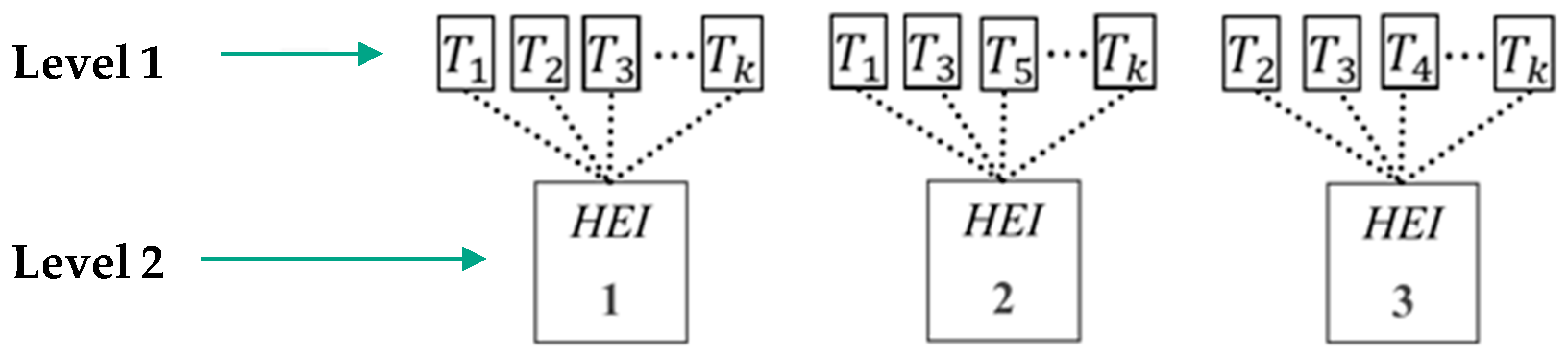
As delineated by Mahmoud et al. [35] and Palardy [36], estimations for nested data, alternatively known as hierarchical regression models, mixed regression models, nested data models, and random coefficient models, are categorized within the realm of Generalized Linear Latent and Mixed Models (GLLAMM). This approach enables the concurrent examination of both fixed and random effects associated with the observed phenomenon.

Data structured using nested relationships are ubiquitous across various human knowledge domains. For instance, patients experiencing heart-related ailments may exhibit nesting in hospitals in which they receive treatment. Moreover, these hospitals could be nested within specific regional contexts in which they operate [37]. Similarly, employees might be nested within their respective departments, which, in turn, can be nested within larger organizational entities such as firms [38]. In both scenarios, the passage of time during patient treatment and the temporal effects on employees could potentially manifest as nested attributes within these individuals [39], showcasing the progression of observations at the individual and/or group levels.

The examples presented illustrate that GLLAMM estimations facilitate the examination of a phenomenon concerning explanatory variables that exhibit variation at the individual observation level while remaining constant across higher levels of nesting without repetition across other superior nesting levels [40,41,42]. Essentially, this form of estimation enables the comprehension of a variable-represented phenomenon in relation to defined predictor variables, wherein alterations may or may not emerge because of delineated nesting structures encompassing recurring measurements stemming from a chronological sequence.

Thus, following Rabe-Hesketh and Skrondal [42], when considering an ordinal categorical phenomenon organized into two levels, the mathematical description of the probability of its occurrence is represented by Equation (12).

$$\mathbb{P}\left(Y_{ij}>m|{\mathbf{X}}_{ij},\mathsf{\alpha },{\mathsf{\nu }}_j\right)=h\left(\mathsf{\beta }{\mathbf{X}}_{ij}+{\mathbf{W}}_{ij}{\mathsf{\nu }}_j-{\mathsf{\alpha }}_m\right)$$

(12)

where $i$ is the subscript representing Level 1 observations; $j$ is the subscript indicating Level 2 observations; $X$ is the $x$-th explanatory variable of the first level; $W$ is the $w$-th second-level predictor variable (therefore invariant for Level 1); and h$\left(.\right)$ is the ordinal logistic cumulative distribution function that represents the cumulative probability of an event.

From Equation (12), we can calculate the probability of observing a category according to Equation (13) [24].

$$\begin{array}{l}\mathbb{P}\left(Y_{ij}>m|,\mathsf{\alpha },{\mathsf{\nu }}_j\right)=\\ \mathbb{P}\left({\alpha }_{m-1}<\mathsf{\beta }{\mathbf{X}}_{ij}+{\mathbf{W}}_{ij}{\mathsf{\nu }}_j+{\epsilon }_{ij}\le {\alpha }_m\right)=\\ \mathbb{P}\left({\alpha }_{m-1}-\mathsf{\beta }{\mathbf{X}}_{ij}-{\mathbf{W}}_{ij}{\mathsf{\nu }}_j<{\epsilon }_{ij}\le {\alpha }_m-\mathsf{\beta }{\mathbf{X}}_{ij}-{\mathbf{W}}_{ij}{\mathsf{\nu }}_j\right)=\\ h\left({\alpha }_m-\mathsf{\beta }{\mathbf{X}}_{ij}-{\mathbf{W}}_{ij}{\mathsf{\nu }}_j\right)-h\left({\alpha }_{m-1}-\mathsf{\beta }{\mathbf{X}}_{ij}-{\mathbf{W}}_{ij}{\mathsf{\nu }}_j\right)\end{array}$$

(13)

where $-\infty \equiv {\alpha }_0\prec {\alpha }_1\prec \cdots \prec {\alpha }_m\equiv +\infty$.

Thus, following Bauer and Sterba [7], a possible theoretical multilevel ordinal logistic model with two levels can be described by expanding Equations (4)–(7) in terms of Equations (14)–(17).

• Level 1:

  $$Z_{m_{ij}}={\alpha }_m-{\beta }_{1j}{X}_{1ij}-\cdots -{\beta }_{kj}{X}_{kij}$$

  (14)

  where $Z_{m_{ij}}$ refers to the logits of an event of interest for the $i$ observations belonging to the group $j$; ${\alpha }_m$ and ${\beta }_{kj}\left(k=1,2,\dots \right)$ refers to the level 1 parameters of the estimation.

• Level 2:

  $${\alpha }_m={\gamma }_{m_{0j}}-{\gamma }_{01}{W}_j-{\nu }_{0j}$$

  (15)

  $${\beta }_{1j}={\gamma }_{10}+{\gamma }_{11}{W}_j+{\nu }_{1j}$$

  (16)

  $$\left(\dots \right)$$

  $${\beta }_{kj}={\gamma }_{k0}+{\gamma }_{kk}{W}_j+{\nu }_{kj}$$

  (17)

  where ${\gamma }_{m_{0j}}$ and ${\gamma }_{kk}$ correspond to the level 2 parameters; ${\nu }_{0j}$ corresponds to the intercept random effects of the second level, and ${\nu }_{kj}$ indicates the slope random effects of level 2.

When the equations for Levels 1 and 2 are combined, the general model described by (18) to (21) is obtained.

• General Model:

$${\mathbb{P}}_{{ij}_{m=1}}=\frac{1}{1+exp\left[-\left({\gamma }_{{m\le 1}_{0j}}-{\gamma }_{01}{W}_j-{\nu }_{0j}-{\gamma }_{10}{X}_{1ij}-{\gamma }_{11}{X}_{1ij}{W}_j-{\nu }_{1j}{X}_{1ij}\cdots -{\gamma }_{k0}{X}_{kij}-{\gamma }_{k1}{X}_{kij}{W}_j-{\nu }_{kj}{X}_{kij}\right)\right]}$$

(18)

$${\mathbb{P}}_{{ij}_{m=2}}=\frac{1}{1+exp\left[-\left({\gamma }_{{m\le 1}_{0j}}-{\gamma }_{01}{W}_j-{\nu }_{0j}-{\gamma }_{10}{X}_{1ij}-{\gamma }_{11}{X}_{1ij}{W}_j-{\nu }_{1j}{X}_{1ij}\cdots -{\gamma }_{k0}{X}_{kij}-{\gamma }_{k1}{X}_{kij}{W}_j-{\nu }_{kj}{X}_{kij}\right)\right]}-{\mathbb{P}}_{{ij}_{m=1}}$$

(19)

$${\mathbb{P}}_{{ij}_{m=3}}=\frac{1}{1+exp\left[-\left({\gamma }_{{m\le 1}_{0j}}-{{\gamma }_{01}{W}_j-\nu }_{0j}-{\gamma }_{10}{X}_{1ij}-{\gamma }_{11}{X}_{1ij}{W}_j-{\nu }_{1j}{X}_{1ij}\cdots -{\gamma }_{k0}{X}_{kij}-{\gamma }_{k1}{X}_{kij}{W}_j-{\nu }_{kj}{X}_{kij}\right)\right]}-{\mathbb{P}}_{{ij}_{m=2}}-{\mathbb{P}}_{{ij}_{m=1}}$$

(20)

$${\mathbb{P}}_{{ij}_{m>3}}=1-{\mathbb{P}}_{{ij}_{m=3}}-{\mathbb{P}}_{{ij}_{m=2}}-{\mathbb{P}}_{{ij}_{m=1}}$$

(21)

Multilevel ordinal logistic regressions can be estimated using the maximum likelihood criterion [42]. For the first level of this type of model, Equation (8) should be followed. For higher estimation levels, the conditional distribution of $Y_j={\left(Y_1,\dots ,Y_J\right)}^{\prime }$ for a set of random effects $j$ is described by Equation (22).

$$f\left(Y_j|\mathsf{\alpha },{\mathsf{\nu }}_j\right)={\prod }_{i=1}^{n_j}{\mathbb{P}}_{ij}^{I_m\left(Y_{ij}\right)}=\exp {\sum }_{i=1}^{n_j}\left[I_m\left(Y_{ij}\right)\log \left({\mathbb{P}}_{ij}\right)\right]$$

(22)

where $I_m\left(Y_{ij}\right)=\left\{\begin{array}{c}1 if Y_{ij}=m\\ 0 \mathrm{otherwise}\end{array}\right.$.

Because the multivariate distribution of ${\mathsf{\nu }}_j$ is assumed to adhere to the Gaussian distribution with mean equal to zero and with the variance matrix $\mathsf{\Theta }$ [43], the contribution of the log-likelihood to nesting above the first level ($L_2$) can be obtained by integrating ${\mathsf{\nu }}_j$ from the joint density function $f\left({\mathbf{Y}}_j,{\mathsf{\nu }}_j\right),$ as shown in Equation (23).

$$\begin{array}{l}{L}_2\left(\mathsf{\beta },\mathsf{\alpha },\mathsf{\Theta }\right)={\left(2\pi \right)}^{-\frac{u}{2}}{\left|\mathsf{\Theta }\right|}^{-\frac{1}{2}}\int f\left({\mathbf{Y}}_j|\mathsf{\alpha },{\mathsf{\nu }}_j\right)\exp \left(-{\mathsf{\nu }}_j^{\mathbf{\prime }}{\mathsf{\Theta }}^{-1}\frac{{\mathit{\nu }}_j}{2}\right)d{\mathsf{\nu }}_j=\\ {\left(2\pi \right)}^{-\frac{u}{2}}{\left|\mathsf{\Theta }\right|}^{-\frac{1}{2}}\int \exp \left[h\left(\mathsf{\beta },\mathsf{\alpha },\mathsf{\Theta },{\mathsf{\nu }}_j\right)\right]d{\mathsf{\nu }}_j\end{array}$$

(23)

where $h\left(\mathsf{\beta },\mathsf{\alpha },\mathsf{\Theta },{\mathsf{\nu }}_j\right)={\sum }_{i=1}^{n_j}\left[I_m\left(Y_{ij}\right)\log \left(p_{ij}\right)\right]-{\mathsf{\nu }}_j^{\mathbf{\prime }}{\mathsf{\Theta }}^{-1}\frac{{\mathit{\nu }}_j}{2}$.

The ordinal logistic models of the GLLAMM family also allow ORs calculations as well as the estimation of intra-class correlations (ICC), which quantifies the extent to which variance at a lower level can be attributed to variability across higher levels (s) [44]. Agresti [23], assuming an ordinal logistic model with two levels, proposed calculating the ICC according to Equation (24).

$$ICC=\frac{{\sigma }_{\nu }^2}{{\sigma }_{\nu }^2+\frac{{\pi }^2}{3}}$$

(24)

where ${\sigma }_{\nu }^2$ indicates the variance of the upper-level errors, and the variance for the first level is approximated by $\frac{{\pi }^2}{3}$ [23,44].

5. Data

The dataset employed in this study comprises an unbalanced panel incorporating repeated measures, encompassing all Brazilian universities listed on the Ranking Web of Universities (WEBOMETRICS (Available at https://www.webometrics.info/en, accessed on 12 July 2023)) from 2012 to 2018. The explanatory variables were obtained from the Brazilian Higher Education Census (CES) (Available at https://www.gov.br/inep/pt-br/areas-de-atuacao/pesquisas-estatisticas-e-indicadores/censo-da-educacao-superior, accessed on 24 September 2023), an initiative run by the country’s Ministry of Education.

The primary aim of WEBOMETRICS is to rank HEIs by assessing their online presence and visibility. Currently, WEBOMETRICS incorporates four indicators that gauge the research and teaching impact of these institutions, reflecting their dissemination of knowledge and resultant influence in terms of university visibility and the consequent impact of this visibility [45]. Essentially, WEBOMETRICS utilizes HEI visibility as a surrogate measure of academic performance.

As per Aguillo et al. [46], the online exposure of institutions is evaluated using comprehensive databases accessed via independent web search engines. These engines, notably Google, Google Scholar, Majestic, Ahrefs, and Scimago Institutions Ranking, are frequently used for cybermetric evaluation. Figure 4 visually represents the documents retrieved from these databases, which were deemed pertinent for inclusion in the ranking process.

The dependent variable involves the categorization of universities into five groups, denoted as $A$, $B$, $C$, $D$ and $E$. These groups were established using a specific methodology: Brazilian universities listed in the WEBOMETRICS ranking for each year of the study were arranged in ascending order based on their respective rankings, that is, from top to bottom. Subsequently, considering the subsets delineated for each year under examination, the original ranking positions of HEIs in WEBOMETRICS were considered. These subsets were further subdivided into five relatively homogeneous segments that were as homogeneous as possible in terms of the number of observations: $A$, $B$, $C$, $D$ and $E$. Universities mentioned only within the ranking in a single year and/or those lacking pertinent data within the CES were subsequently excluded.

Table 1. The distribution of the number of Brazilian HEIs in the strata proposed by the research.

Year	Number of Universities					Total
	$\mathit{A}$Group	$\mathit{B}$Group	$\mathit{C}$Group	$\mathit{D}$Group	$\mathit{E}$Group
2012	38 (20.7%) (14.6%)	37 (20.1%) (14.4%)	35 (19.1%) (14.3%)	37 (20.1%) (14.3%)	37 (20.1%) (15.0%)	184 (100.0%) (14.5%)
2013	38 (20.4%) (14.6%)	38 (20.4%) (14.4%)	36 (19.4%) (14.8%)	38 (20.4%) (14.7%)	36 (19.4%) (14.6%)	186 (100.0%) (14.7%)
2014	37 (20.4%) (14.2%)	37 (20.4%) (14.4%)	35 (19.3%) (14.3%)	37 (20.4%) (14.3%)	35 (19.3%) (14.2%)	181 (100.0%) (14.3%)
2015	37 (20.3%) (14.2%)	37 (20.3%) (14.4%)	36 (19.8%) (14.8%)	37 (20.3%) (14.3%)	35 (19.2%) (14.2%)	182 (100.0%) (14.4%)
2016	37 (20.3%) (14.2%)	37 (20.3%) (14.4%)	36 (19.8%) (14.8%)	37 (20.3%) (14.3%)	35 (19.2%) (14.2%)	182 (100.0%) (14.4%)
2017	37 (20.4%) (14.2%)	37 (20.4%) (14.4%)	35 (19.3%) (14.3%)	37 (20.4%) (14.3%)	35 (19.3%) (14.2%)	181 (100.0%) (14.3%)
2018	37 (21.8%) (14.2%)	34 (20.0%) (13.2%)	31 (18.2%) (12.7%)	35 (20.6%) (13.6%)	33 (19.4%) (13.4%)	170 (100.0%) (13.4%)
Total	261 (20.6%) (100.0%)	257 (20.3%) (100.0%)	244 (19.3%) (100.0%)	258 (20.4%) (100.0%)	246 (19.4%) (100.0%)	1266 (100.0%) (100.0%)

provides an overview of the distribution of HEIs across the groups.

Thus, in Table 1, the HEIs in Group $A$ represent the best-placed Brazilian academies in the WEBOMETRICS ranking, whereas the universities in Group $E$ represent the worst placed in the ranking. Table 1 also shows the imbalance in the repeated measures panel used in this study.

Table 2. Description of the research’s predictor variables.

Variable	Description
$year$	Year of monitoring of a given Brazilian university, considering the period from 2012 to 2018.
$hei\_code$	Unique identifier of a given Brazilian university.
$hei\_names$	Name of university.
$is\_federal$	Nominal dichotomous variable that identifies the stratum if a given Brazilian university is, or is not, a university mostly maintained with Federal funds (Legally, Brazil comprises three types of universities: public universities (Federal, State, and Municipal), private non-profit universities (typically affiliated with religious entities), and private for-profit universities [48]. Broadly, Federal universities in Brazil are esteemed as the most prestigious; however, notable exceptions exist in international rankings, notably USP and the University of Campinas (UNICAMP), which are State universities [49]).
$rate\_doctoral\_prof$	Metric variable that relates the number of students enrolled in the institution’s doctoral programs (doctoral students and Ph.D. candidates) to the total number of professors at a given Brazilian university.

lists the explanatory variables selected for the estimations.

With this context in mind, this tutorial aims to investigate a particular construct: can the performance of Brazilian universities, considering performance as the position (strata A to E) in the WEBOMETRICS ranking, be concurrently elucidated over time, the proportion of students engaged in doctoral programs concerning the total count of professors, and the classification of an HEI as a federal university?

Table 3. Univariate descriptive statistics of the study variables.

Metric Variables
Variable	Min	1stQ	Median	3rdQ	Max	Mean	SD
$rate\_doctoral\_prof$	0.000	0.006	0.099	0.326	2.719	0.265	0.410
Categorical Variables
$is\_federal$				yes: 405; no: 861.

Note: 1stQ stands for first quartile; 3rdQ stands for third quartile; and SD stands for standard deviation.

shows the univariate descriptive statistics for the study’s metric variables and the frequency tables for the survey’s categorical variables.

Given the above explanations, the model considered the context of the passage of time nested in each university, as shown in Figure 5.

The next section presents the models considered in this study.

6. Empirical Application

A total of four models were estimated: two of them using arbitrary recoding and/or arbitrary dichotomization approaches, both from the GLM family, respectively a classical linear regression model (Linear GLM) and a binary logistic model (Binary GLM); the other two estimations correspond to ordinal logistic regressions, the first being from the GLM family, and the other GLLAMM (Ordinal GLM and Ordinal GLLAMM, respectively).

For the Linear GLM model, the dependent variable was assumed to be a metric, considering classes $E$ to $A$ in the study as values from $1$ to $5$, as follows: $E=1$, $D=2$, $C=3$, $B=4$, and $A=5$. It could be argued that, for this type of estimation, the use of regression techniques for discrete variables (for example, Poisson, Gamma, Poisson-Gamma) would be more useful, as discussed in Section 5, in which the proposition of classes from $E$ to $A$ in the research was made by prioritizing the homogeneity of the number of HEIs in each category. As such, calculating the density probability of the phenomenon, when in metric form, would show a curve similar to that of a uniform distribution, creating difficulties for the regression models for the count data mentioned above.

However, for the Binary GLM estimation, groups $A$ and $B$ were joined to form a new stratum called “$best performance$”. The groups $D$ and $E$ were combined to create a “$worst performance$” stratum. For this model, the individuals in the Group $C$ were considered to be missing values.

Finally, for the ordinal models (Ordinal GLM and Ordinal GLLAMM), the dependent variable was considered in accordance with Section 5; that is, considering all groups from $E$ to $A$, categorically and in that precise order.

Table 4. Transformations applied to the study’s dependent variable.

Estimation	Transformation Applied to the Dependent Variable
Ordinal GLM	None. The dependent variable is the same as described in Section 5, i.e., groups ordered in ascending order from E to A.
Ordinal GLLAMM	Same as above.
Linear GLM	The consideration of groups ordered in ascending order from E to A in metric form, taking values from 1 to 5.
Binary GLM	Combining groups A and B to form the best_performance category; combining strata D and E to create the worst_performance category; disregarding the observations belonging to Group C.

summarizes the transformations proposed for the dependent variable of the research, depending on the model generated.

Table 5. The algorithms and packages used in the research.

Estimation	Algorithm	Package	Version
Linear GLM	lm()	stats	4.3.0
Binary GLM	glm()	stats	4.3.0
Ordinal GLM	clm()	ordinal	2023.12-4
Ordinal GLLAMM	clmm()	ordinal	2023.12-4

shows the algorithms, packages, and their respective versions in the R computer language. The codes and databases can be found in the Supplementary Materials.

Table 6. Comparison of the calculated parameters of the study’s regression models.

Parameters	Linear GLM Coefficients	Binary GLM Coefficients	Ordinal GLM Coefficients	Ordinal GLLAMM Coefficients
${threshold}_E$	-	-	−0.95857 (0.13414)	−4.72308 (0.53377)
${threshold}_D$	-	-	0.34030 (0.13000)	1.87845 (0.32800)
${threshold}_C$	-	-	1.56304 (0.13852)	6.93229 (0.00204)
${threshold}_B$	-	-	3.73099 (0.18940)	12.81046 (0.00314)
$intercept$	2.41243 (0.06940)	−1.35809 (0.20318)	-	-
$year$	−0.03336 b (0.01498)	−0.14496 a (0.04641)	−0.11248 a (0.02767)	−0.12914 a (0.00163)
$rate\_doctoral\_prof$	1.86460 a (0.07720)	11.18187 a (0.91810)	7.10328 a (0.38711)	12.78852 a (0.00313)
$is\_federal$	0.77469 a (0.06760)	0.88002 a (0.22474)	0.83859 a (0.13499)	6.19182 a (1.02605)
$Var\left({\nu }_{0j}\right)$	-	-	-	54.3560
${\chi }_{Wald}^2$	−747.7575 * (d.f. = 3)	−651.1707 (d.f. = 3)	−982.7719 (d.f. = 3)	−106.3296 (d.f. = 3)
$LL$	−1863.838 (d.f. = 5)	−382.7152 (d.f. = 4)	−1.545.69700 (d.f. = 7)	−770.28320 (d.f. = 8)
$ICC$	-	-	-	0.94293
$n$	1266	1022	1266	1266

Note: Var and LL refer to the variances of the random effects and log-likelihood, respectively. ^a Significance level of 0.01. ^b Significance level of 0.05. * For linear models of the GLM family, the F-statistic is commonly used, which in this case indicates $F=338.700$, with three degrees of freedom for the regression and 1.262 degrees of freedom for the residuals.

compares the parameters of the estimates produced by this study. In Table 6, the first three columns show the parameters of the models that only consider the fixed effects of the predictor variables on the phenomenon studied, while the last column shows the model from a multilevel perspective, that is, considering fixed effects and random intercept effects simultaneously. For the Ordinal GLLAMM estimation, there was no algorithmic convergence for the estimation of the slope random effects.

Table 6 provides the mathematical transcriptions of the GLM models and GLLAMM estimation, which considers fixed effects and random intercept effects. For didactic reasons, in the case of ordinal models, we present the equations for calculating the probability of class; after all, for the other classes, it would be enough to change the values of the intercepts.

• Linear GLM estimation:

$$Y_i=2.41243-0.03336{year}_i+1.86460{rate\_doctoral\_prof}_i+0.77469{is\_federal}_i$$

(25)

• Binary GLM estimation:

$${\mathbb{P}}_{{m=1}_i}=\frac{1}{1+exp\left[-\left(-1.35809-0.14496{year}_i+11.18187{rate\_doctoral\_prof}_i+0.88002{is\_federal}_i\right)\right]}$$

(26)

• Ordinal GLM estimation:

$${\mathbb{P}}_{{m=E}_i}=\frac{1}{1+exp\left[-\left(-0.95857+0.11248{year}_i-7.10328{rate\_doctoral\_prof}_i-0.83859{is\_federal}_i\right)\right]}$$

(27)

• GLLAMM estimation:

$${\mathbb{P}}_{{m=E}_{ij}}=\frac{1}{1+exp\left[-\left(-4.72308-{\nu }_{0j}+0.12914{year}_{ij}-12.78852{rate\_doctoral\_prof}_{ij}-6.19182{is\_federal}_{ij}\right)\right]}$$

(28)

The next section presents discussions and comparisons of the models proposed by the research.

7. Comparison of Research Models and Discussion

The analysis of the results presented in Table 6 begins with the statistics ${\chi }_{Wald}^2$. This statistical metric serves a similar purpose to the likelihood-ratio test (LR test) [42], seeking to compare the researchers’ final model with its null model analog using the same dependent variable and the same number of observations. Mathematically, the calculation of the statistic is described by Equation (29):

$$-2\times \left({LL}_{model}-{LL}_{null model}\right)$$

(29)

The $H_0$ of the test described by (29) indicates that there are no statistically significant differences between a given research model and its respective null model. The results are presented in

Table 7. ${\chi }_{Wald}^2$ results.

Comparing Estimates	${\mathit{\chi }}_{\mathit{W}\mathit{a}\mathit{l}\mathit{d}}^2$	d.f.	p-Value
Linear GLM versus a null linear GLM estimation	747.7315	2	0.000
Binary GLM versus a null binary logistic GLM estimation	651.1707	3	0.000
Ordinal GLM versus a null ordinal logistic GLM estimation	982.7719	3	0.000
Ordinal GLLAMM versus a multilevel null ordinal logistic estimation	106.3296	3	0.000

.

According to the results shown in Table 7, it can be said that all the research models were statistically different from their analogous null estimates at a 1% significance level, i.e., the phenomenon as a function of the intercept only. In other words, the results in Table 7 reinforce that at least one predictor variable, ceteris paribus, proved to be statistically different from zero for all models.

Subsequently, a second round of LR tests [50,51] was proposed to check which of the estimations in Table 6 best suited the research data, that is, the modeling of the rankings of Brazilian universities in WEBOMETRICS. Thus, the value of ${\chi }_{LR test}^2$, in order to check whether the $LL$ gain between two different models is statistically equal to zero, is calculated by adapting expression (29), described by Equation (30).

$$-2\times \left({LL}_{model 1}-{LL}_{model 2}\right)$$

(30)

Using Equation (30), all the $LL$ values from all the models shown in Table 6 were compared with each other pair by pair. The $H_0$ of the discussed LR test is that the two models compared are not statistically different from each other; however, $H_1$ indicates that a given estimate is more appropriate for the case studied. The LR test results are presented in

Table 8. LR test results.

Comparative Estimates	$\mathit{L}\mathit{L}$	${\mathit{\chi }}_{\mathit{L}\mathit{R}\mathit{t}\mathit{e}\mathit{s}\mathit{t}}^2$	d.f.	p-Value
Linear GLM versus Binary GLM	-	-	-	-
Linear GLM versus Ordinal GLM	−1863.838 −1545.697	636.2818	2	0.000
Linear GLM versus Ordinal GLLAMM	−1863.838 −770.2827	2187.111	3	0.000
Binary GLM versus Ordinal GLM	-	-	-	-
Binary GLM versus Ordinal GLLAM	-	-	-	-
Ordinal GLM versus Ordinal GLLAMM	−1545.697 −770.2827	1550.829	1	0.000

.

In Table 8, it is not possible to present the results of the LR tests involving Binary GLM estimation because of the difference in the sampling considered by the models (see Table 6). In any case, Section 7.2 discusses Binary GLM estimation as well as the problems with the methodological choice of disregarding the observations present in Group $C$. It is also true that Section 7.4 will compare the accuracies of all the models, as well as considerations regarding the non-parametric Kolmogorov–Smirnov Predictive Accuracy (KSPA) test [52], to verify the adequacy of the estimates for the phenomenon studied.

In the next section, discussions and considerations regarding the GLM Linear estimation are discussed.

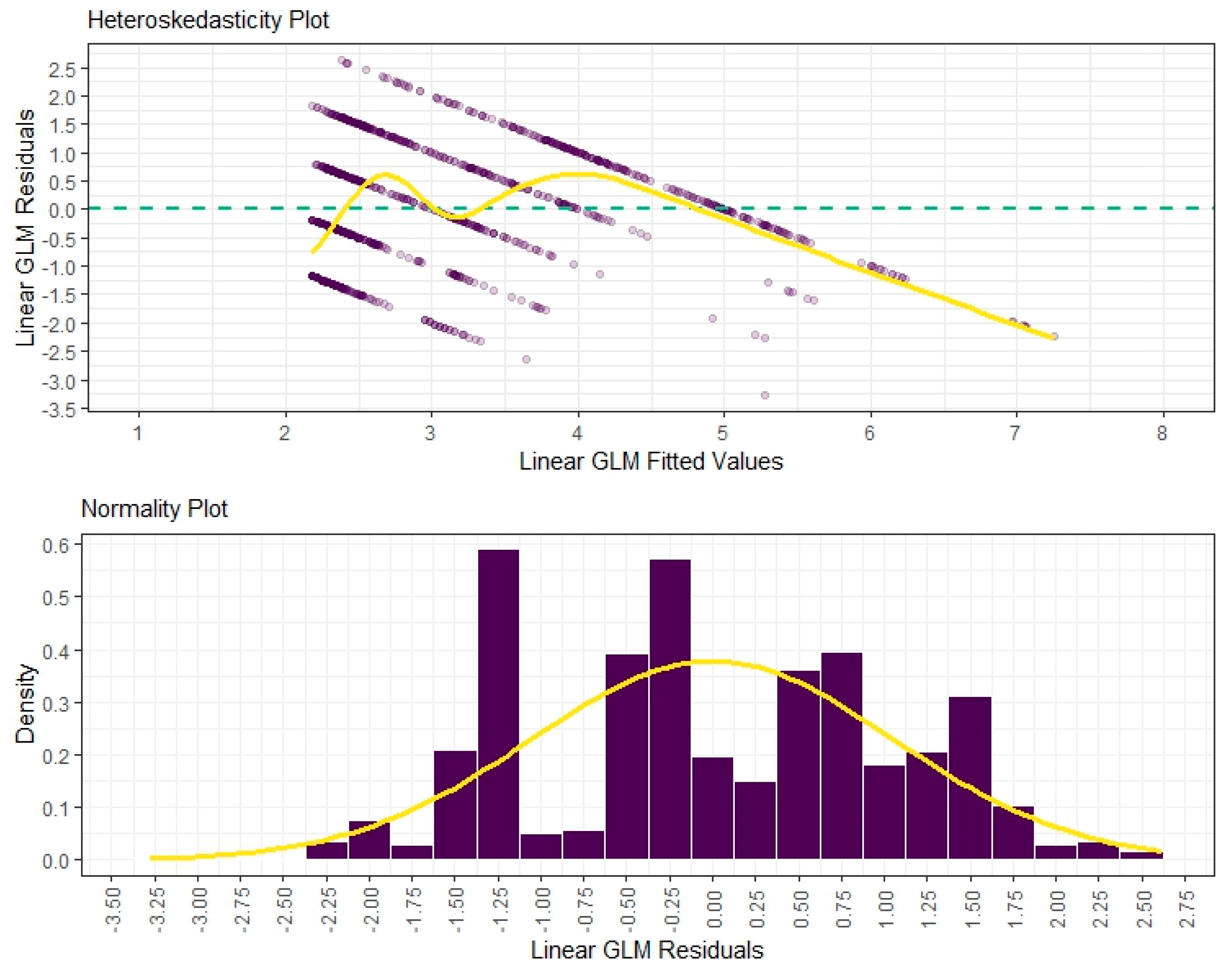
7.1. The GLM Linear Estimation

At this point, it should be remembered that, for didactic purposes, the survey’s dependent variable, which is ordinal categorical, was arbitrarily recoded to a metric specification, where 1 indicates stratum $E$ HEIs, and 5 indicates Group $A$ HEIs (see Table 4).

From the analysis of the parameters of the Linear GLM model with its intercept, as shown in Table 6 and in Equation (25), it can be seen that this model is optimistic in generating difficulties for any HEI to be classified in a category lower than $D$, given its value of $2.41243$. In other words, even if all predictor variables were mathematically equal to 0, the GLM Linear estimation would not classify any HEI in the Group $E$ of the research. According to Table 1, 246 individuals belong to the aforementioned stratum $E$.

Table 6 also shows that an increase in one unit in the variable year would cause a reduction of −0.03336 in the measurement of the dependent variable, and all other conditions remain constant. On the other hand, if the HEI was a federal university ($is\_federal=1$), the dependent variable would receive an increase of 0.77469 in its unit of measurement, ceteris paribus; if it was not a federal university ($is\_federal=0$), the increase would be equal to zero, while the other conditions remaining constant. Finally, an increase in one unit in the variable would lead, ceteris paribus, to an increase of 1.86460 in the dependent variable.

It is interesting to note that although the maximum value of the dependent variable studied for the GLM Linear model is mathematically equal to 5 (which represents the Group $A$ of HEIs), there were 76 observations with their respective fitted values greater than 5. The highest fitted value recorded was approximately 7.25, whereas the lowest fitted value recorded was approximately 2.18.

The estimation of fitted values that extrapolate the observed values, given the occurrence of arbitrary recoding for a given variable to be assumed as a metric, is expected in the literature. Both Bauer and Sterba [7] and Long and Freese [53] agree that arbitrary metric recoding for an ordinal phenomenon can generate fitted values below or above the categories existing in the phenomenon. The authors also pointed out that, as the fitted values extrapolate (upward or downwards) the observed values, there is a compression of the variability of the residues, generating the problems of heteroscedasticity and non-adherence of the residues to normality.

In fact, the postulates by Bauer and Sterba [7] and Long and Freese [53] regarding the condition of homoscedasticity and the non-existence of adherence to the normality of the residuals were observed in the Linear GLM estimation of the research.

To confirm this, the Breusch-Pagan test (BP test) was performed to verify the absence of heteroscedasticity [54]. The $H_0$ of this test indicates that the assumption of homoscedasticity for GLM linear regressions is met. Because ${\chi }_{BP}^2=48.004$, with 3 degrees of freedom, we have a p-value = 0.000. Therefore, it can be said that the Linear GLM model is heteroscedastic at a 1% significance level. The upper portion of Figure 6 illustrates the situation described above.

The Shapiro-Francia normality test (SF test) was also performed to check whether the assumption $\epsilon ~N\left(0,{\sigma }^2\right)$ was met [55]. The $H_0$ indicates adherence to the Gaussian distribution for a given significance level. Because $W_{SF}=0.97568$, with the respective p-value = 0.000, it can be said that in the GLM Linear estimation, its residuals do not adhere to normality at the 1% significance level. The lower part of Figure 6 illustrates this situation.

More than that predicted by Bauer and Sterba [7] and Long and Freese [53], the researchers noted the existence of autocorrelation in the residuals of the Linear GLM model. The Durbin-Watson test (DW test) was used to diagnose the autocorrelation of the error terms [56], where the $H_0$ indicates the non-existence of the situation discussed for a given significance level. The DW test indicated the presence of autocorrelation in the residuals of the Linear GLM estimation for up to 9-time lags at a 1% significance level.

Below are some considerations and discussions regarding the Binary GLM model.

7.2. The GLM Binary Estimation

Before discussing the interpretability of the parameters of the Binary GLM estimation, it should be recalled that the ordinal polytomous dependent variable with five levels was dichotomized, as shown in Table 4.

Binary models require the phenomenon of a dichotomous nature, which is where the crossroads began for the authors of the study. Groups $B$ and $A$ were assumed to be the upper strata of the database, forming the $best performance$ group, while groups $E$ and $D$ were combined to form the $worst performance$ category.

However, the researchers understand that if the intention of the modeling was to support the managerial decision-making process, whether of a policymaker or a university manager, this decision would raise questions that would be difficult to answer.

▪

If the intention is to try to study, based on the variables present in the database, which factors lead an HEI to be in the top positions of the WEBOMETRICS ranking (Group $A$, in this case), why should the stratum $A$ be mixed with the stratum $B$?

▪

On the other hand, if the intention is to understand what leads an HEI to fall into the very bottom positions of the ranking studied, why mix group $D$ with stratum $E$?

▪

However, if the intention is to study the composition of the Group $B$ or the Group $D$, what should be performed with the HEIs in the groups $A$, $C$, and $E$?

▪

If we assume the conjunction of groups $B$ and $A$, forming a new category, and the mixture of $D$ and $E$ generating another category, what should we do with the individuals in the Group $C$?

To illustrate the problems that can be generated by the chosen path, it was decided to disregard the individuals in the Group $C$, i.e., missing values were considered. To do so, 244 rows of the database were not used to train the algorithm. In other words, the model’s supervised learning was deprived of information on 244 individuals.

The analysis of the parameters of a logistic model, be it binary, ordinal, or multinomial, unlike a classic linear regression model, is based on the calculation of ORs. As such, it can be said that according to Table 6, the Binary GLM estimation indicates that the chance of a federal university being considered part of the $best performance$ group (strata $B$ and $A$) is 2411 times greater ($e^{0.88002}$) compared to an HEI that is not a federal university, ceteris paribus. However, there is no way to determine whether such an HEI will be classified into the original groups $B$ or $A$.

Table 6 also indicates that a one-unit increase in the variable $rate\_doctoral\_prof$, with all other conditions held constant, increases the chance of a given HEI being categorized as $best performance$ Group by 71,816.53 times ($e^{11.18187}$). Finally, with regard to the variable year, the passage of one year, ceteris paribus, decreases the chance of a university being inferred as the $best performance$ category by 13.49%, i.e., it must be multiplied by a factor of 0.8651, since $e^{-0.14496}=0.8651$.

7.3. The GLM and GLLAMM Ordinal Estimations

7.3.1. OR Analysis

Following Table 6, according to the Ordinal GLM estimation, the chance of a Brazilian academy, other than a federal university, being in Group $E$, of the WEBOMETRICS ranking is 2.313 times greater ($e^{0.83859}$) than federal universities. However, for the estimation that considers both fixed and random effects (Ordinal GLLAM), the chance of a Brazilian university, other than a federal academy, being classified in the Group $E$ must be multiplied by a factor of 488.735 ($e^{6.19182}$), i.e., 487.7% higher than that for a federal university.

The proposed interpretation can also be achieved via the predicted probabilities of different values $m$ when $is\_federal=0$ versus $is\_federal=1$, as presented in

Table 9. Predicted probability that a given Brazilian university will occupy performance groups $E$ to $A$, whether or not it is a federal university.

Model	Federal University	Group E Probability	Group D Probability	Group C Probability	Group B Probability	Group A Probability
GLM	No	0.2771637	0.3070985	0.2425269	0.1498028	0.02340802
	Yes	0.1421969	0.2357452	0.2956447	0.2738828	0.05253039
GLLAMM	No	0.00880949216	0.85862298	0.1315927	0.0009720858	0.000002732045
	Yes	0.00001818504	0.01319328	0.6638869	0.3215682073	0.001333463391

.

From Table 9, and using Equation (9), when comparing the probabilities of a given Brazilian HEI being in $E$ group, because it is not a federal university against the fact that it is a federal university, we have:

• For Ordinal GLM estimation:

$$\frac{\frac{0.2771637}{\left(1-0.2771637\right)}}{\frac{0.1421969}{\left(1-0.1421969\right)}}\approx 2.313$$

• For Ordinal GLLAMM estimation:

$$\frac{\frac{0.00880949216}{\left(1-0.00880949216\right)}}{\frac{0.00001818504}{\left(1-0.00001818504\right)}}\approx 488.733$$

Still, on the results in Table 9, if the attempt at analysis was based on the question of what the chance of a Brazilian HEI, being a federal university, being categorized in the $D$ or $C$ or $B$ or $A$ strata, and not being categorized in the $E$ stratum, we would still have:

• For Ordinal GLM estimation:

$$\frac{\frac{\left(0.2357452+0.2956447+0.2738828+0.05253039\right)}{\left[1-\left(0.2357452+0.2956447+0.2738828+0.05253039\right)\right]}}{\frac{\left(0.3070985+0.2425269+0.1498028+0.02340802\right)}{\left[1-\left(0.3070985+0.2425269+0.1498028+0.02340802\right)\right]}}\approx 2.313$$

• For Ordinal GLLAMM estimation:

$$\frac{\frac{\left(0.01319328+0.6638869+0.3215682073+0.001333463391\right)}{\left[1-\left(0.01319328+0.6638869+0.3215682073+0.001333463391\right)\right]}}{\frac{\left(0.85862298+0.1315927+0.0009720858+0.000002732045\right)}{\left[1-\left(0.85862298+0.1315927+0.0009720858+0.000002732045\right)\right]}}\approx 488.733$$

Another way of analyzing the variable $is\_federal$, following the estimation proposed in Table 6 and Equations (27) and (28), is to directly calculate the chance of a Brazilian HEI being categorized in the Group $E$, being a federal university. The answer to this question would be $e^{-0.83859}=0.43232$, all other conditions being equal. In other words, for Ordinal GLM modeling, the chance of a Brazilian federal academy being categorized in group E must be multiplied by a factor of 0.43232; that is, it is 56.768% lower than if this HEI were not a federal university, ceteris paribus.

On the other hand, when proposing the previous question for the Ordinal GLLAMM estimation, the chance of a Brazilian HEI being categorized in the Group $E$, being a federal university, should be multiplied by a factor of 0.00205 ($e^{-6.19182}$), i.e., for the GLLAMM estimation, it would be 99.795% lower than if this HEI were not a federal university, with other conditions remaining constant.

When looking at the time span considered by the variable $year$, it is interesting to note that, according to the results in Table 6, the estimated coefficients are close for both models. In the case of the estimation presented in (27), adding one unit to the variable year increases the chance of a given Brazilian university being categorized in the stratum E by 13.785% ($e^{0.12914}$), ceteris paribus. In the case of the model in (28), the passage of one year implies an increase in the chance of a given Brazilian HEI being categorized in the stratum $E$ of 11.905% ($e^{0.11248}$), ceteris paribus.

Finally, when generating an increment of one unit in the variable $rate\_doctoral\_prof$, the Ordinal GLM modeling—Equation (27)—points out that the chance of a given Brazilian HEI being classified in the Group $E$ is 99.917% lower ($e^{-7.10328}$). The Ordinal GLLAMM estimation indicates that this chance is 99.999% lower ($e^{-12.78852}$).

7.3.2. Intercept (Threshold) Analysis

Another important point is the possibility of analyzing the intercepts of the models as well as the differences between the intercepts of the estimates proposed by the research.

In the case of the ordinal logistic regressions in the survey (Ordinal GLM and Ordinal GLLAMM), the first consideration to make is that the intercept values indicate the probability of a given Brazilian HEI being categorized in any stratum proposed by the survey (from $E$ to $A$) when the other predictor variables are equal to 0. These probabilities for the data studied can be found in rows 1 and 3 of Table 9.

Table 9 also explains the problem of not considering the observational idiosyncrasies of the data. The calculated probabilities, in the case of the Ordinal GLM estimation (see row 1 of Table 5), are more evenly distributed between the groups $E$, $D$, $C$, and $B$. In other words, the Ordinal GLM model is optimistic for those HEIs that have low values of the variable $rate\_doctoral\_prof$, guaranteeing easier predictions of reasonable ratings in the WEBOMETRICS ranking (e.g., $C$ or $B$) for this type of university.

On the other hand, when a similar analysis is carried out for the Ordinal GLLAMM estimation (see line 3 of Table 9), its probability distributions between the groups adopted by the research leave homogeneity aside and penalize universities with low values of the variable $rate\_doctoral\_prof$ more heavily. It is also true that, in this case, the Ordinal GLLAMM model also penalizes, considerably, the predictions of positions in the WEBOMETRICS ranking for HEIs that are not federal universities, which leads to the discussion of the consideration of random effects, which must be analyzed on a case-by-case basis. This implies that the intercepts proposed by the Ordinal GLLAMM model must be corrected using the values of their random effects (${\nu }_{0j}$), as presented in Appendix A, following the logic of ${\gamma }_{m_{0j}}-{\nu }_{0j}$ (28). The values are therefore adjusted to the values of the GLLAMM estimation thresholds, made because of the peculiarities and observational nesting, for the intercepts of the multilevel model.

As previously mentioned, the values are presented in Appendix A of this study. Therefore, when considering the Ordinal GLLAMM estimation for the two levels modeled, the intercept for Group $E$, in the case of the Federal University of Western Pará (UFOP), presented in the first line of

Table A1. Calculated values of ${\nu }_{0j}$ for the individuals in the research.

HEI Names	Is It a Federal University?	${\mathit{\nu }}_{0\mathit{j}}$
Federal University of Western Para	yes	−14.99009635
Federal University of The Southern Border	yes	−13.73180070
Darcy Ribeiro North Fluminense State University	no	−13.67610299
Federal University of Latin American Integration	yes	−13.51506685
University of the International Integration of Afro-Brazilian Lusophony	yes	−13.27160473
Federal University of Health Sciences of Porto Alegre	yes	−10.37416534
Sao Francisco University	no	−9.752614271
Catholic University of Petropolis	no	−9.506667313
Municipal University of Sao Caetano Do Sul	no	−9.215742952
University of the Sapucai Valley	no	−9.123246743
Federal University Of Lavras	yes	−8.436202000
Vila Velha University	no	−8.411085314
Nilton Lins University	no	−8.354072711
Candido Mendes University	no	−8.347125089
Marilia University	no	−8.234944757
Cuiaba University	no	−8.232441189
Metropolitan University of Santos	no	−8.188602961
Amapa State University	no	−8.079419237
State University of Health Sciences of Alagoas	no	−8.064994723
Severino Sombra University	no	−8.064994723
Santa Ursula University	no	−8.064994723
Presidente Antonio Carlos University	no	−8.064994723
Camilo Castelo Branco University	no	−8.064994723
Iguacu University	no	−8.064994723
Ibirapuera University	no	−8.064994723
Vale do Rio Doce University	no	−8.064994723
Planalto Catarinense University	no	−8.064994723
State University of Rio Grande Do Sul	no	−8.064994723
Rio Verde University	no	−8.064994723
State University of Roraima	no	−8.064994723
State University of Alagoas	no	−8.064994723
University of the Campanha Region	no	−7.974555746
Braz Cubas University	no	−7.974555746
Itauna University	no	−7.860477850
Federal University of Amapa	yes	−7.677428376
Grande ABC University	no	−7.174835087
Jose do Rosario Vellano University	no	−6.468046656
Joinville Region University	no	−6.242757024
Federal University of Roraima	yes	−6.143240450
State University of Northern Parana	no	−6.006872575
Cruz Alta University	no	−5.891714847
Federal Rural University of the Amazon	yes	−5.795563090
Cruzeiro do Sul University	no	−5.657494653
Foundation Federal University of Grande Dourados	yes	−5.334567978
Catholic University of Salvador	no	−5.089159010
Federal University of Triangulo Mineiro	yes	−5.007426154
Federal Rural University of The Semi-Arid Region	yes	−4.281043460
Federal University of the Jequitinhonha and Mucuri Valleys	yes	−4.252152738
Federal University of Alfenas	yes	−3.731053337
Sorocaba University	no	−3.492989706
Federal University of Itajuba	yes	−3.298113673
Anhanguera University	no	−3.133556781
Federal University of Acre	yes	−2.978102075
Dom Bosco Catholic University	no	−2.976272160
Franca University	no	−2.805512911
Federal Rural University of Pernambuco	yes	−2.636823118
Salgado de Oliveira University	no	−2.629415418
Ribeirao Preto University	no	−2.601152707
Potiguar University	no	−2.475139817
Federal Rural University of Rio De Janeiro	yes	−2.434885013
Sagrado Coracao University	no	−2.421717770
Acarau Valley State University	no	−2.386904761
Tocantins University	no	−2.386904761
Rondonia Federal University	yes	−2.321180703
Federal University of The Sao Francisco Valley	yes	−2.268085483
Pontifical Catholic University of Sao Paulo	no	−2.203539879
Santos Catholic University	no	−2.185315550
Federal University of Alagoas	yes	−2.143302503
Bandeirante University of Sao Paulo	no	−2.123308368
Federal University of the State of Rio De Janeiro	yes	−2.080315766
Federal University of Tocantins Foundation	yes	−1.859696753
Pampa Federal University Foundation	yes	−1.700680157
Tuiuti University Of Parana	no	−1.658723722
Professor “Jose De Souza Herdy” University of Grande Rio	no	−1.652905607
Mogi Das Cruzes University	no	−1.619034111
Fumec University	no	−1.516993675
State University of Mato Grosso Do Sul	no	−1.436778710
City of Sao Paulo University	no	−1.424392798
Sao Judas Tadeu University	no	−1.415667314
Minas Gerais State University	no	−1.007623742
Regional University of Cariri	no	−0.936288606
Reconcavo da Bahia Federal University	yes	−0.889593824
Rio Verde Valley University	no	−0.866415961
State University of Piaui	no	−0.866415961
Santa Cecilia University	no	−0.866415961
Amazonia University	no	−0.383843188
State University of Campinas	no	0.000001716
Federal University of Rio Grande Do Sul	yes	0.000441941
University of Sao Paulo	no	0.001643641
Federal University of Rio De Janeiro	yes	0.026150447
Federal University of Minas Gerais	yes	0.085981454
Federal University of Santa Catarina	yes	0.091604285
University of Western Paulista	no	0.126200469
Federal University of Ceara	yes	0.294389265
Federal University of Sao Carlos	yes	0.310381033
Federal University of Rio Grande	yes	0.343443136
State University of Maranhao	no	0.485721407
Federal University of Pernambuco	yes	0.547950963
University of Western Santa Catarina	no	0.576139939
Castelo Branco University	no	0.630102533
Santo Amaro University	no	0.630102533
Contestado University	no	0.630102533
Federal University of Vicosa	yes	0.822644994
Federal University of Sao Paulo	yes	0.919583062
Brasilia University	yes	1.214990312
ABC Federal University	yes	1.272662705
Methodist University of Piracicaba	no	1.299548471
Positivo University	no	1.455745927
Paraiba Valley University	no	1.553119688
Federal University of Parana	yes	1.624846845
Federal University of Pelotas	yes	1.638422371
Federal University of Mato Grosso	yes	1.884384028
Mato Grosso State University	no	1.939326056
Catholic University of Pernambuco	no	2.036981661
Federal University of Piaui	yes	2.120003238
Federal University of Maranhao	yes	2.139401048
Amazonas State University	no	2.336524924
Federal University of Ouro Preto	yes	2.394441009
Regional University of Northwestern Rio Grande do Sul State	no	2.616960817
Technological Federal University of Parana	yes	2.619387447
Tiradentes University	no	2.622135482
Federal University of Mato Grosso Do Sul	yes	2.632919886
Federal University of Bahia	yes	2.876477055
Julio de Mesquita Filho Paulista State University	no	3.132439958
Federal University of Campina Grande	yes	3.140551802
North Parana University	no	3.439539019
Guarulhos University	no	3.574697821
Para State University	no	3.587890006
Uberaba University	no	3.729799680
Federal University of Rio Grande Do Norte	yes	3.999376018
Federal University of Amazonas	yes	4.036775310
Federal University of Sergipe	yes	4.067316504
Feevale University	no	4.121768718
Federal University of Santa Maria	yes	4.145951484
Federal University of Sao Joao Del Rei	yes	4.185864581
Veiga de Almeida University	no	4.203584165
Anhembi Morumbi University	no	4.301687824
Rio Grande do Norte State University	no	4.318800807
Paranaense University	no	4.318800807
Community University of the Chapeco Region	no	4.318800807
Alto Uruguai e das Missões Integrated Regional University	no	4.345878060
Federal University of Para	yes	4.491504554
Taubate University	no	4.634044812
Federal University of Uberlandia	yes	4.804616760
Fluminense Federal University	yes	4.852823692
Federal University of Paraiba	yes	4.985137105
Santa Cruz State University	no	5.038850317
State University of Southwest Bahia	no	5.041621224
Salvador University	no	5.164845860
State University of Midwest	no	5.309082320
Pontifical Catholic University Of Goias	no	5.457353354
State University of Ceara	no	5.626526798
Paulista University	no	5.709381079
Federal University of Goias	yes	5.752312579
State University of Goias	no	5.802286719
University of Extreme South Catarinense	no	5.833866187
Federal University of Juiz De Fora	yes	5.948009565
Santa Cruz do Sul University	no	6.024406003
Regional University of Blumenau	no	6.220647133
Federal University of Espírito Santo	yes	6.229696268
Catholic University of Pelotas	no	6.237231979
Pontifical Catholic University of Rio de Janeiro	no	6.599206352
Rio dos Sinos Valley University	no	6.699586880
Mackenzie Presbyterian University	no	6.703518715
Fortaleza University	no	7.200753664
Itajai Valley University	no	7.296747253
Lutheran University Of Brazil	no	7.47832689
Pernambuco University	no	7.481812386
Bahia State University	no	7.512211886
Brazilian Catholic University	no	7.566038025
State University of Western Parana	no	7.654403455
Pontifical Catholic University Of Rio Grande Do Sul	no	7.961440315
Nove de Julho University	no	7.996981951
Pontifical Catholic University of Campinas	no	8.087346315
State University of Feira de Santana	no	8.281796599
Rio de Janeiro State University	no	8.606858437
Santa Catarina State University	no	8.611956177
Ponta Grossa State University	no	8.637562072
Caxias do Sul University	no	8.711704534
Methodist University of Sao Paulo	no	8.908381972
Paraiba State University	no	9.227040499
Pontifical Catholic University of Minas Gerais	no	9.310656616
University of Southern Santa Catarina	no	9.448175941
State University Of Maringa	no	9.515227693
Estacio de Sa University	no	9.615633159
Passo Fundo University	no	10.12255267
State University of Montes Claros	no	11.46164999
State University of Londrina	no	11.51611222
Pontifical Catholic University of Parana	no	12.82779457

, should not be considered equal to $-4.72308$ (see Table 6), but equal to $-4.72308-(-14.975500)=10.25242$.

The next section discusses the accuracy and suitability of these estimates.

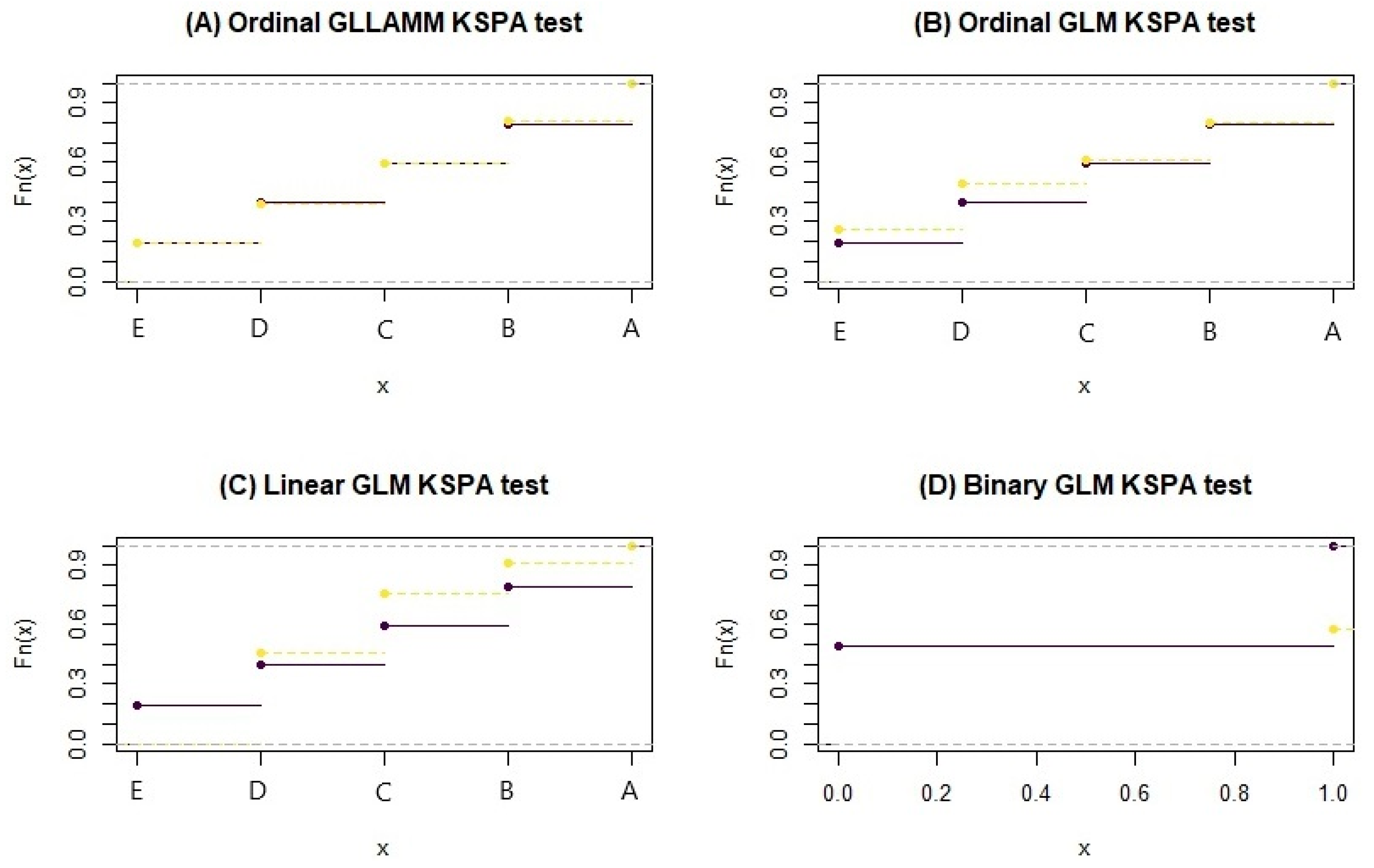
7.4. Accuracy and Suitability of Estimates

Different modeling methodologies typically employ specific techniques to measure the accuracy. In the case of classic regression models, the R² statistic is commonly utilized for this purpose [57], as well as the mean squared error (MSE) or root mean square error (RMSE), among others [58]. Binary logistic models make it possible to propose confusion matrices by assuming some cutoff (including analyses of sensitivity, specificity, etc.), as well as calculating the area under the ROC curve or the Gini coefficient [12,23]. Finally, ordinal logistic models usually assume, according to the trained algorithm, the category with the highest probability of occurrence, and the classification error or hit rate is evaluated. As these methods of measuring accuracy between models are considerably different, it was decided to adapt all estimates so that they could be evaluated in terms of classification accuracy rates.

Figure 7 shows the cross between the observed (abscissa axis) and predicted categories (ordinate axis). From this image, it would be difficult to advocate disregarding the nesting present in the study data by presenting the intersections between predicted classes and observed classes for the research estimates, considering the possibility of a guess for each model.

To measure the accuracy of the models, considering a single guess from Figure 7, we simply calculate the sum of its main diagonal and divide the result by the total sample. Therefore, the Ordinal GLLAMM estimation has an accuracy of $\frac{232+216+210229+235}{1266}=\frac{1122}{1266}\approx 88.63\%$, whereas for the Ordinal GLM estimation, we have an accuracy of $\frac{204+91+43+84+155}{1266}=\frac{577}{1266}\approx 45.58\%$.

The lowest accuracy was observed in the Linear GLM model, with ($\frac{101+54+104+183+0}{1266}=\frac{442}{1266}\approx 34.91\%$. This value was obtained by considering fitted values greater than 5 to be equal to 5 (group $A$).

This difference in predictive power between the Ordinal GLM and Ordinal GLLAMM models can be explained using the ICC value of the Ordinal GLLAMM estimate. For the aforementioned model, the calculated ICC was 94.29%; that is, 94.29% of the total variability in the performance of the Brazilian HEIs studied was related to changes between HEIs (correlations within repeated measurements of ranking classes).

The Binary GLM estimation achieved an accuracy of $\frac{394+462}{1022}=\frac{856}{1022}\approx 83.76\%$. However, it should be remembered that 244 observations were disregarded in the modeling, and groups were combined to create a dichotomous phenomenon, and there is no way of predicting which of the groups assumed by the study (from $E$ to $A$) a given Brazilian HEI might be classified in.

A non-parametric KSPA test [52] was used for all the estimations. According to the authors, the KPSA test allows the distances between the cumulative distributions (CDF) of the observed values and the predicted values to be measured without being impacted by any autocorrelation that may be present in the forecast errors. The $H_0$ of the KSPA test proposes that two samples (in this case, the observed values from the database and the predicted values from each model) belong to the same CDF at a given significance level. The results of the KSPA test are summarized in

Table 10. KSPA test results.

Estimation	KSPA Test	p-Value
Ordinal GLLAMM	0.0134	0.6335
Ordinal GLM	0.0901	0.000
Linear GLM	0.1651	0.000
Binary GLM	0.0802	0.000

.

Table 10 suggests, at the 1% significance level, that the predictions of the GLM models are not suitable for this case, ceteris paribus. Figure 8 shows the CDF distances between the observed values (purple and solid dashes) and the predicted values (yellow dashed color) of the research estimates.

Therefore, Figure 8 reinforces the suitability of the Ordinal GLLAMM estimation for the data studied. The following is a discussion of the expected values of the phenomenon as a function of the predictor variables of the study.

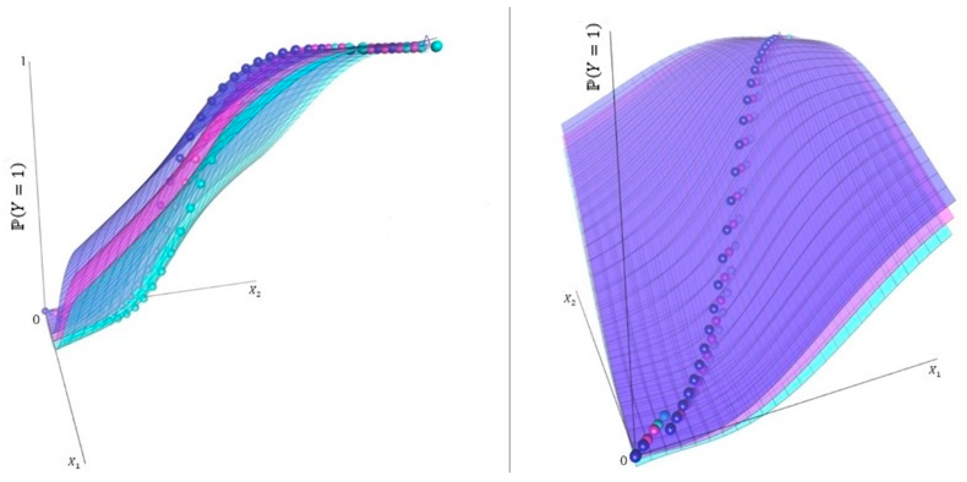
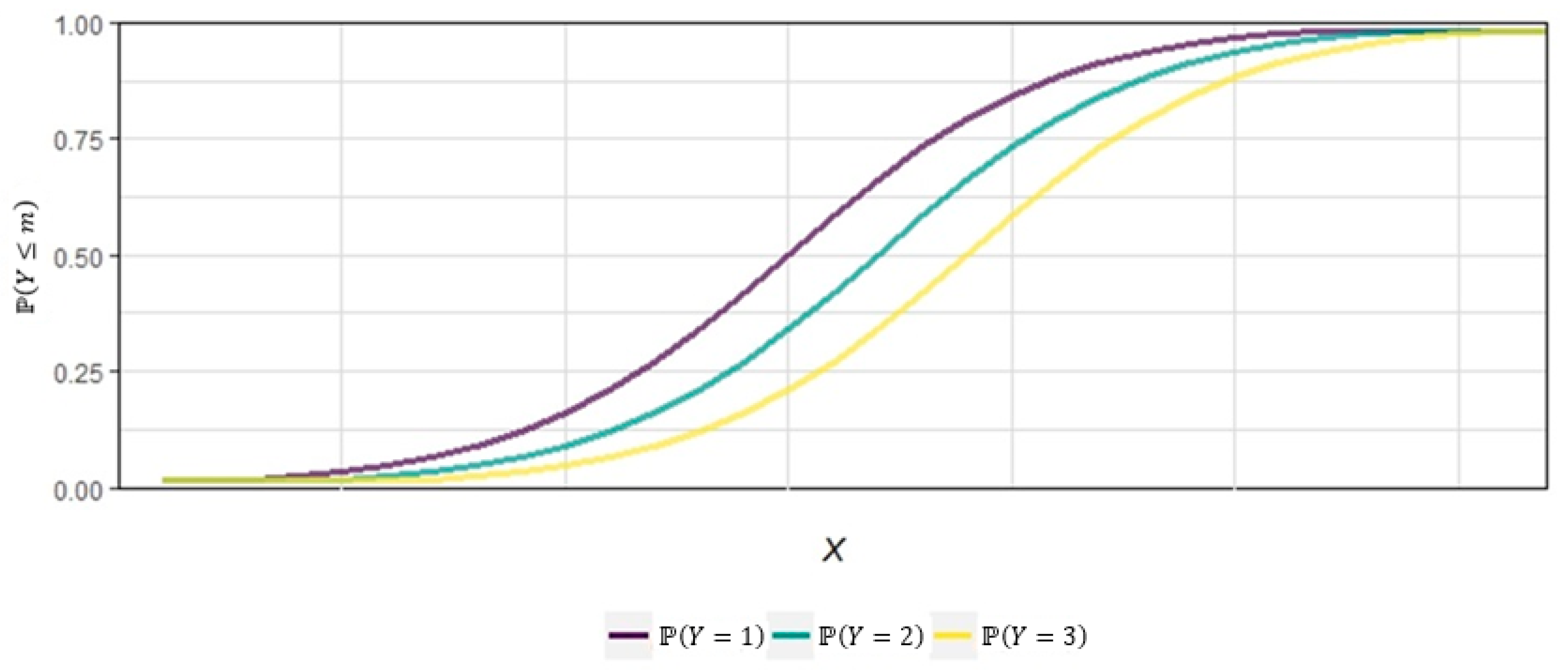
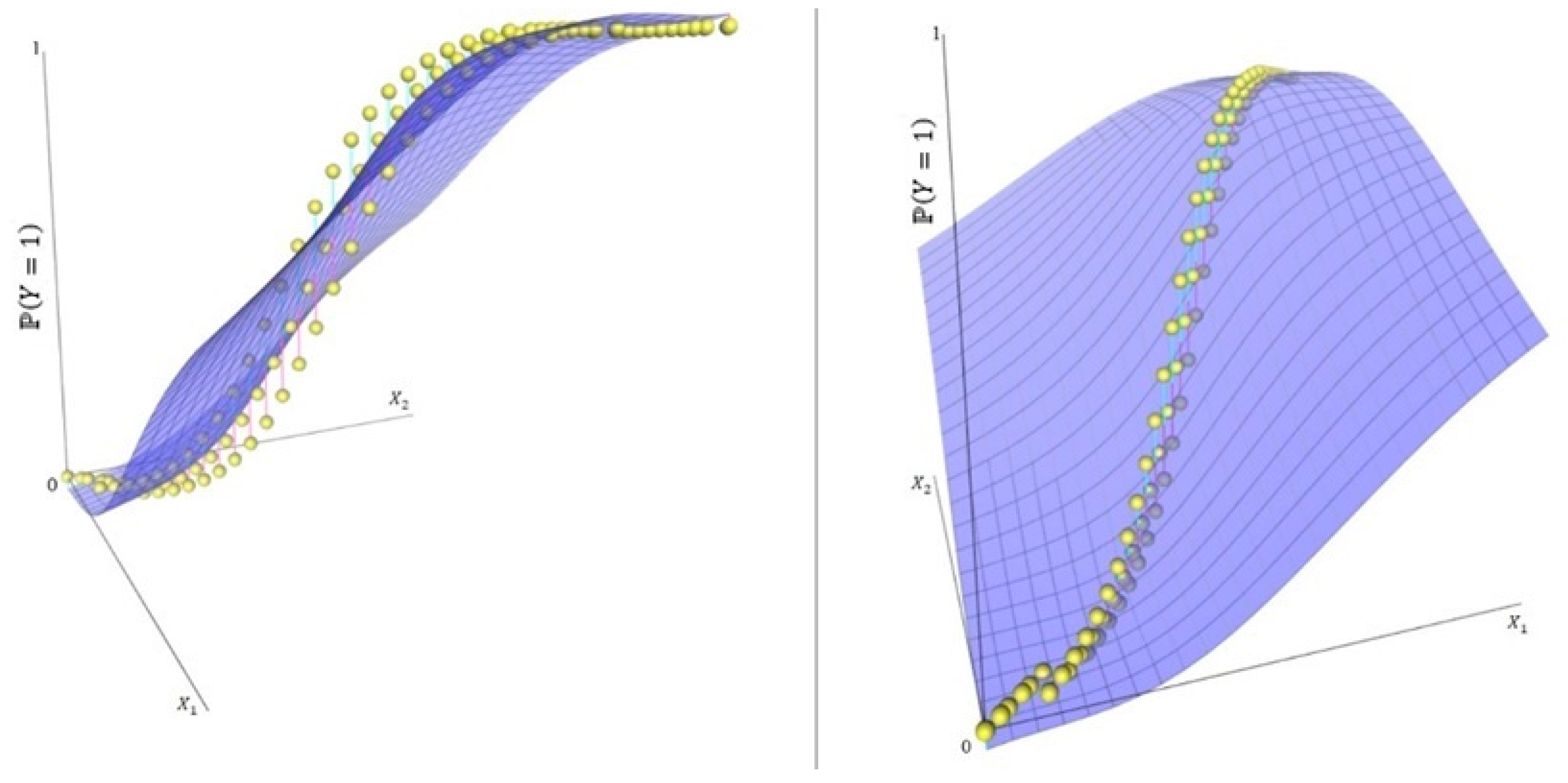
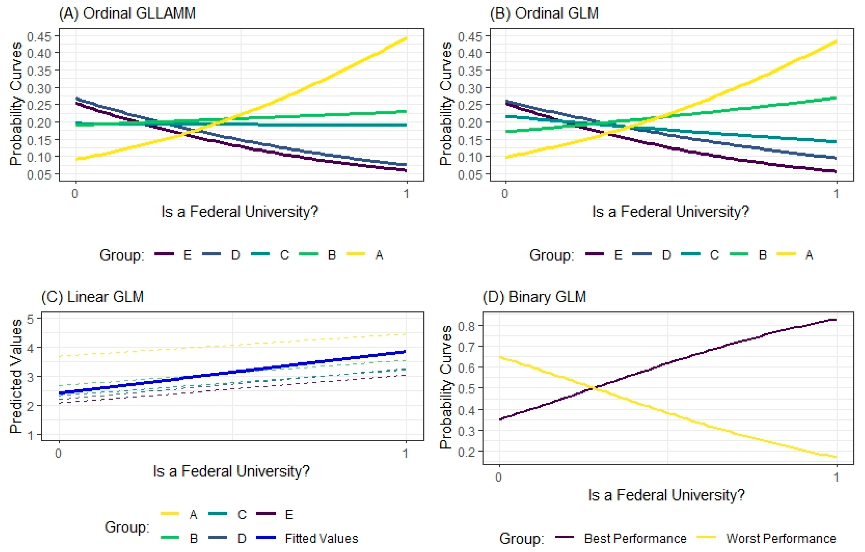
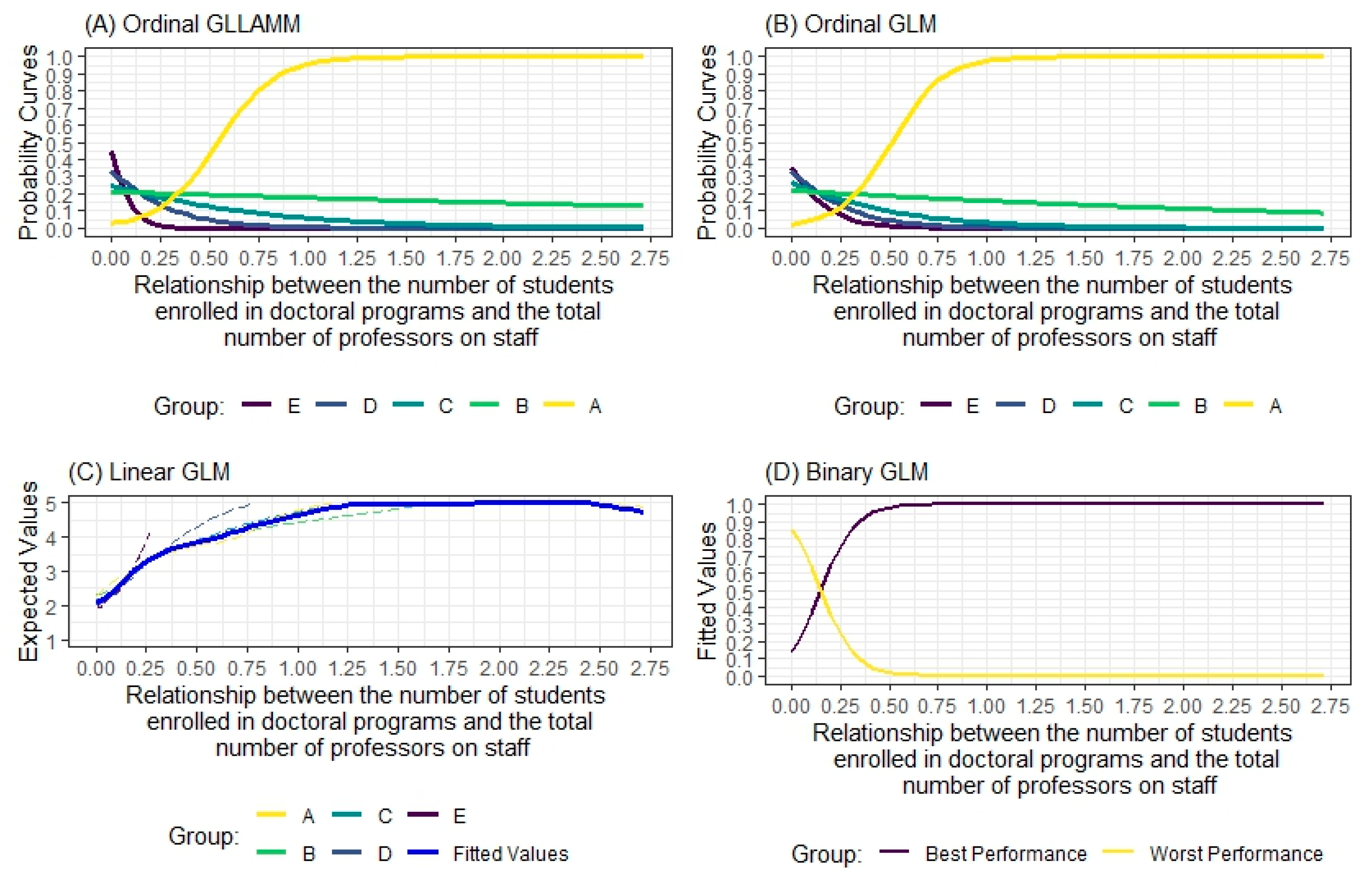
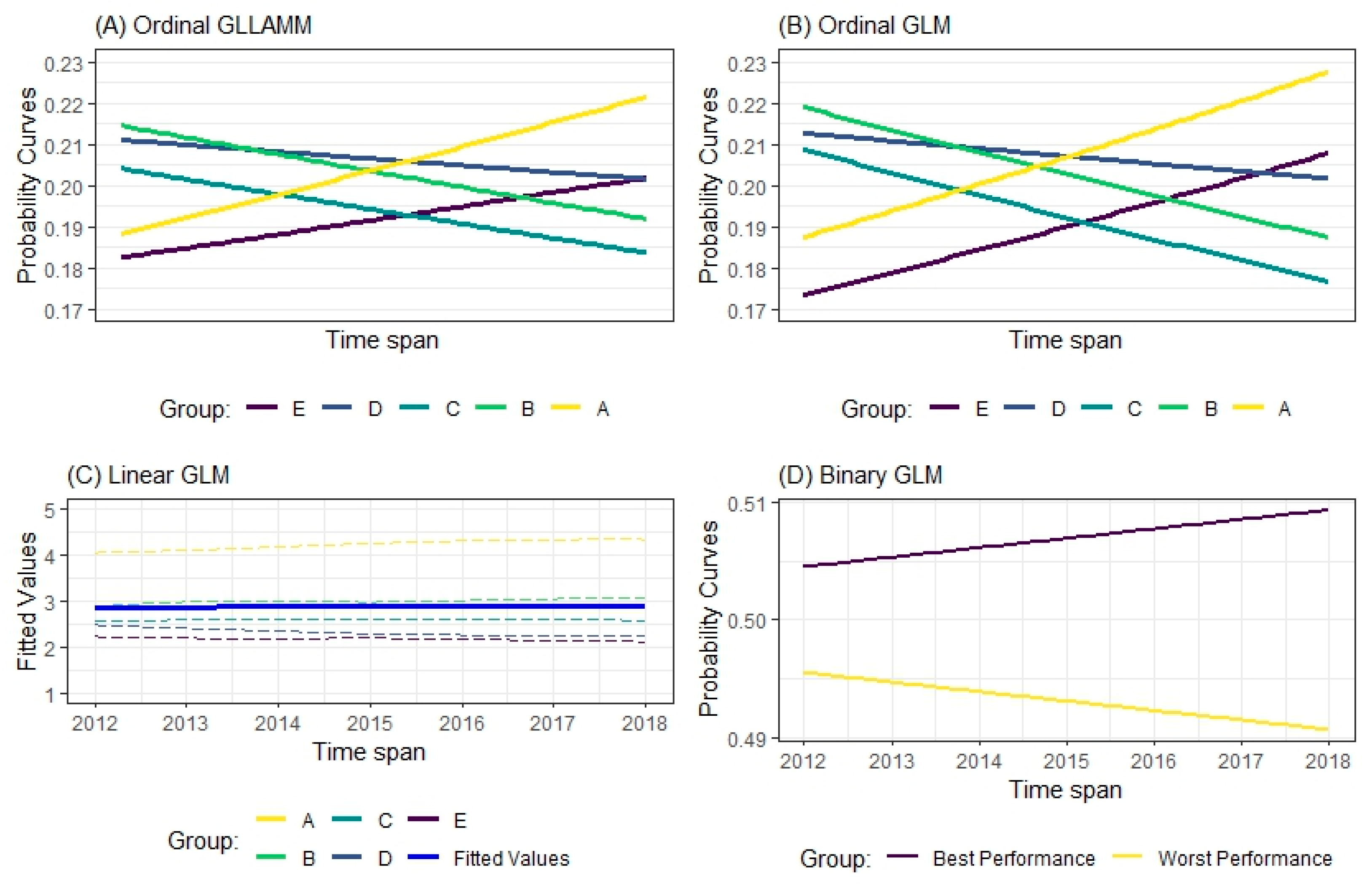
7.5. The Expected Values as a Function of the Study’s Predictor Variables

Figure 9, Figure 10 and Figure 11 show the estimated probability curves for the Ordinal GLLAMM, Ordinal GLM, and Binary GLM models, respectively that Section 7.2 and Section 7.3 deal with variations in the probability of occurrence of the phenomenon for the models discussed, and not their probabilities of occurrence for each category of the dependent variable.

Figure 9, Figure 10 and Figure 11 also show the behavior of the fitted values of the Linear GLM model as a function of each of the predictor variables used in the study. Section 7.1 presented the marginal effects of each explanatory variable on this phenomenon. In this section, we present the fitted values for the Linear GLM model (solid blue curve) as well as the fitted values for each Group of HEIs that were assumed by the research.

Figure 9 shows that when Ordinal GLLAMM, Ordinal GLM, and Binary GLM estimations are adopted, the fact that a Brazilian HEI is a federal university increases its likelihood of being classified in the upper strata of the research.

According to Figure 9, ceteris paribus, for the Ordinal GLLAM estimation, it is also true that there is a certain probability that the university in question, even though it is a federal university, will be classified in strata $B$ or $C$ and probably there will be no classification in strata $D$ or $E$. On the other hand, other conditions remain constant; for the Ordinal GLM model, the growth rate of the probability curve of a given federal university being considered to belong to category $B$ is higher compared to the Ordinal GLLAM estimation, as well as a higher decay rate for the probability of a given federal university being considered in Group $C$, compared to the Ordinal GLLAMM estimation.

As shown in Figure 9, when looking at the behavior of the probability curves of the Binary GLM model, the probability of a given HEI being considered part of the upper strata of the research (B and A), being a federal university, exceeds 80%, ceteris paribus. However, the model points out that the fact that a Brazilian HEI is not a federal university can cause it to be classified in the lower strata of the study ($E$ and $D$) with a probability of approximately 65%, all other conditions remaining constant.

The biggest problem with the Binary GLM estimation observed in this study is that the simplification of the phenomenon, thanks to an arbitrary dichotomization, together with the disregard of almost 20% of the observations in the database, creates a false sense of ease in interpreting the model’s results. For this estimation, nothing is known about what makes an HEI in Group $A$ different from an HEI in Group $B$ in terms of increases or decreases in the explanatory variables of the research—the same can be said for groups $D$ and $E$.

More incisively, from the researchers’ perspective, by assuming arbitrary dichotomization in place of a phenomenon that manifests itself in an ordinal polychotomous way, there is disregard for the extremes of the phenomenon assumed to be original. There is no way to understand what led a given HEI to be in the top positions in the ranking studied and, as such, no way for the HEIs in an immediately lower group to understand what needs to be performed for them to climb up the WEBOMETRICS rankings. The opposite is also true; that is, there is no way to diagnose the reasons why a given HEI has been categorized as group E, and therefore, little could be performed to help it.

It could be argued that if the Binary GLM model indicates the important variables for achieving the $best performance$ category, then it would be sufficient to apply the same conditions abstracted from it to universities belonging to the $worst performance$ group. The fallacy of this argument lies in the fact that it ignores that there is an unknown distance between category $A$ and category $B$, as well as observational idiosyncrasies; the same can be said between categories $B$ and $C$, whose distances are unknown (in fact, category $C$ was disregarded by the estimate discussed), as well as differences in regional, social, political, and economic realities, and so on, up to category $E$.

The behavior of the Linear GLM model, as shown in Figure 9, also indicates a tendency for Brazilian federal universities to be classified in the highest groups of HEIs. However, the interpretability of the Linear GLM model in this case is the most intricate. It has already been discussed that the Linear GLM estimation did not classify any HEI in the stratum $E$, but there is also the difficulty of establishing a cutoff point that indicates the point from which the change in category will be considered.

What is meant is that starting from the two-dimensional visualization proposed in Figure 9, imagine that a given HEI has a calculated fitted value of 2.5. Strictly speaking, a priori, the Linear GLM model would not have considered this observation as part of category $D$, nor as part of category $C$—but rather, the estimation would classify this HEI somewhere between these two groups. The data analyst would be left with the arbitrary decision of “adjusting” the model’s prediction (i.e., some kind of rounding) so that it converges on the categories being studied—something similar to what the researchers did in Section 7.1 because, for 76 observations, there were fitted values greater than 5.

However, for researchers, this attitude seems to go against the reasons why a machine learning model exists or is estimated. If the central idea of modeling is to support the decision-making process, regardless of the field of science being considered and regardless of the activity being observed, the estimation discussed would help less (not to say that it would be in the way) in deciding on a certain course of action in relation to the other models in the study. This situation occurred, it must be stressed, due to the arbitrary recoding of the ordinal categorical dependent variable so that it could take on metric values and, therefore, so that a classical linear regression algorithm could be trained.

Figure 10 shows that small values of the ratio of students involved in doctoral programs to the total number of professors can lead to an average probability of 45%, ceteris paribus, of a Brazilian HEI being classified as a stratum $E$, according to the Ordinal GLLAM estimation. According to the Ordinal GLM model, this average probability drops to approximately 35% on average, and all the other conditions are equal.

Figure 10 also demonstrates that, for the Ordinal GLM estimation, values close to 0 and 0.1 of the $rate\_doctoral\_prof$ variable do not differentiate the classification of a given Brazilian HEI in the $E$, $D$, $C$ and $B$ strata. However, the situation narrated occurs to a lesser extent for the Ordinal GLLAM model.

In addition, according to Figure 10, the Ordinal GLLAM and Ordinal GLM estimates, $rate\_doctoral\_prof=0.50$ indicate an average probability of approximately 50% for a given Brazilian HEI to be predicted in the stratum $A$. For the same modeling, the values of $rate\_doctoral\_prof>0.75$ points to a given university being considered in the stratum $A$ with an average probability of more than 85%, ceteris paribus.

On the other hand, according to the Binary GLM estimation and its results are shown in Figure 10, values of $rate\_doctoral\_prof>0.25$ would already be a strong indicator for a given Brazilian university to appear in the upper strata of the WEBOMETRICS ranking. Linear GLM estimation indicates that the higher the value of the $rate\_doctoral\_prof$ variable, the greater the possibility of an HEI moving up the categories, and when $rate\_doctoral\_prof\ge 1.25$, ceteris paribus, a given HEI should be placed in the stratum $A$ of the study.

In Figure 11, in relation to the Ordinal GLLAMM and Ordinal GLM models, it can be said that the passage of time benefits universities at the extremes of classification—groups $E$ and $A$, with higher growth rates in the case of the Ordinal GLM estimation. It is also true that Ordinal GLM estimation has higher decay rates for predicting groups $D$, $C,$ and $B,$ when compared to Ordinal GLLAMM estimation. Although there is little mathematical difference in the values of the slope coefficient for the variable year (see Equations (27) and (28)), the fact that the Ordinal GLLAMM estimation considers observational idiosyncrasies may justify the smoother growth and decay rates, depending on the case.

In the case of the Linear GLM estimation, according to Figure 11, the passage of time seems to benefit HEIs in groups $B$ and $A$; to harm universities in groups $D$ and $E$, and not to change the status of HEIs belonging to Group $C$. According to Figure 11, the model’s general fitted values (solid blue line) indicate a slight downward trend in the categorization of Brazilian universities over time.

Finally, for Binary GLM modeling, the passage of time is perceived as beneficial for universities in the top stratum and detrimental for HEIs in the other Group. However, according to Figure 11, the changes in the classification probabilities, ceteris paribus, were small.

8. Final Considerations

In this study, we demonstrated the application of proportional odds-type ordinal logistic regression to assess the impact of incorporating both fixed and random effects when predicting the rankings of Brazilian universities using an unprecedented, real-world database that is now freely available to the academic community.

The research also compared the proportional odds-type ordinal logistic regression (GLM and GLLAMM) estimates with a classic linear regression model and with a binary logistic regression model, using the following construct: Can the performance of Brazilian universities, considering performance as in the WEBOMETRICS ranking, be concurrently elucidated over time, the proportion of students engaged in doctoral programs concerning the total count of professors, and the classification of an HEI as a Brazilian federal university? All codes in the R computer language have been provided and are commented in English for teaching purposes.

The Ordinal GLLAMM estimation showed the highest accuracy of all models (88.63% correct; see Section 7.4 and Figure 7). The Binary GLM model achieved 83.76% accuracy, the Ordinal GLM estimation showed 45.58% accuracy, and the Linear GLM model showed the lowest accuracy of all the estimations in the study (34.91%).

When comparing the Binary GLM and Ordinal GLLAMM models, it should be noted that the dependent variable in the binary logistic estimation underwent transformations to dichotomize the phenomenon under study [5]. Groups B and A of the dependent variable formed the “best performance” group, while the combination of strata D and E generated the “worst performance” category. The estimates for Group C were missing values, totaling 244 observations.

In this sense, the considerable accuracy of the Binary GLM model tells us a lot about the HEIs grouped according to the extremes of the strata studied, but it does not tell us anything about what makes a given Brazilian university belong to Group C.

This may be of interest to the HEIs originally grouped in stratum A to maintain the status quo of their performance level, but it does not seem to help other universities. For example, when using the Binary Model, an HEI belonging to group B would extract little information on how to climb positions and would know little (or almost nothing) about falling to a position belonging to stratum C. On the subject of the Binary Model, a given HEI originally belonging to group E would have little understanding of the factors that keep it from the top positions in the ranking, given that its information was mixed with stratum D and the model discussed, knowing nothing about the central position in the ranking, the C group. In our view, the use of Binary GLM estimation in this case could generate a cult of real-world performative average mediocrity.

However, when looking at the so-called Linear GLM model, it should be remembered that the phenomenon in this case was assumed to be a discrete metric, with a value from 1 (for group E) to 5 (for stratum A) [4]. For the dataset studied, this estimation generated 76 fitted values greater than 5 [7,53], forcing the researchers to consider these observations as members of group A. For the case studied, the Linear GLM model was not capable of categorizing observations in stratum E. In the case of the Linear GLM model, it was also found that its residuals did not adhere to normality, heteroscedasticity, and autocorrelation for up to nine lags, at 1% significance, ceteris paribus [7,53,54,55,56,57,58].

When comparing the Ordinal GLM and Ordinal GLLAMM models, the study’s findings suggest that due to the oversight of observational intricacies, particularly within the GLM model, in contrast to the GLLAMM model, there was an inability to comprehend the diverse contexts encountered by the HEIs featured in the dataset, resulting in the lower accuracy observed. Furthermore, the calculated ICC of 94.29% within a panel database incorporating repeated measures served as a robust indicator of the heterogeneous behavior evident within the observations.

Nevertheless, it is important to emphasize that this scientific article adopts a tutorial format, explicitly avoiding any assertion that the enclosed models comprehensively encapsulate a wide array of realities within Brazilian Higher Education Institutes (HEIs). Brazil is well known for its extensive heterogeneity across various dimensions and is particularly highlighted by its stark income inequality. This socioeconomic disparity inevitably exerts a profound influence on the development trajectory of educational institutions, regardless of whether they are public or private or government funding.

Moreover, the manner in which the researchers categorized Brazilian universities into groups E to A is subject to limitations, much like other methodological approaches. For any subsequent researcher intending to further this study, determining the appropriate distribution of universities across categories, as well as establishing the optimal number of categories for stratification, presents itself as a set of challenges to be addressed.

Indeed, the genuine intent of the researchers engaged in this study in disseminating the discussed guidelines for ordinal logistic estimations, along with the R programming language code, is to encourage further exploration. The aspiration is for subsequent research endeavors to delve deeper, encompassing both multilevel perspectives and the accurate handling of ordinal categorical data.

In situations where researchers encounter challenges in explicitly identifying existing contexts (nestings) in their data, the suggested approach involves generating clusters based on the observations themselves. This can encompass methodologies such as centroid-based/partition clustering, hierarchical clustering, and fuzzy-based clustering. It is plausible that the resultant groupings could be regarded as latent nestings, facilitating the estimation of the random effects. However, it is important to acknowledge that cluster analysis is an unsupervised technique. If the outcomes are integrated into a multilevel model, the predictive capacity of the model may be lost. Nonetheless, these results offer more precise diagnostic insights into the researchers’ dataset.

Continuing from the preceding suggestion, to avoid losing the predictive power of ordinal regression, it may make sense to show unobservable nesting. For example, the use of classificatory Support Vector Machines, or if the amount of data is not a problem, the use of deep artificial neural networks aimed at classifying observations could serve as viable strategies.

References

1. Lalla, M. Fundamental characteristics and statistical analysis of ordinal variables: A review. Qual. Quant. 2017, 51, 435–458. [Google Scholar] [CrossRef]
2. Vogt, W.P.; Johnson, R.B. The SAGE Dictionary of Statistics & Methodology: A Nontechnical Guide for the Social Sciences, 5th ed.; SAGE Publications: London, UK, 2015. [Google Scholar]
3. Kampen, J.; Swyngedouw, M. The Ordinal Controversy Revisited. Qual. Quant. 2000, 34, 87–102. [Google Scholar] [CrossRef]
4. Fullerton, A.S.; Anderson, K.F. Ordered Regression Models: A Tutorial. Prev. Sci. 2023, 24, 431–443. [Google Scholar] [CrossRef]
5. Liddell, T.M.; Kruschke, J.K. Analyzing ordinal data with metric models: What could possibly go wrong? Exp. Soc. Psychol. 2018, 79, 328–348. [Google Scholar] [CrossRef]
6. Nadler, J.T.; Weston, R.; Voyles, E.C. Stuck in the Middle: The Use and Interpretation of Mid-Points in Items on Questionnaires. J. Gen. Psychol. 2015, 142, 71–89. [Google Scholar] [CrossRef] [PubMed]
7. Bauer, D.J.; Sterba, S.K. Fitting multilevel models with ordinal outcomes: Performance of alternative specifications and methods of estimation. Psychol. Methods 2011, 16, 373–390. [Google Scholar] [CrossRef] [PubMed]
8. Hedeker, D.; Gibbons, R.D. A Random-Effects Ordinal Regression Model for Multilevel Analysis. Biometrics 1994, 50, 933. [Google Scholar] [CrossRef]
9. Fielding, A.; Yang, M.; Goldstein, H. Multilevel ordinal models for examination grades. Stat. Model. 2003, 3, 127–153. [Google Scholar] [CrossRef]
10. Li, B.; Lingsma, H.F.; Steyerberg, E.W.; Lesaffre, E. Logistic random effects regression models: A comparison of statistical packages for binary and ordinal outcomes. BMC Med. Res. Methodol. 2011, 11, 77. [Google Scholar] [CrossRef]
11. Hedeker, D. Methods for Multilevel Ordinal Data in Prevention Research. Prev. Sci. 2015, 16, 997–1006. [Google Scholar] [CrossRef]
12. Hilbe, J.M. Logistic Regression Models; CRC Press: Boca Raton, FL, USA, 2014. [Google Scholar]
13. Fernandes, A.J.; Shukla, B.; Fardoun, H. Indian Higher Education in World University Rankings—The Importance of Reputation and Branding. J. Stat. Appl. Probab. 2022, 11, 673–681. [Google Scholar] [CrossRef]
14. Liu, A.; He, H.; Tu, X.M.; Tang, W. On testing proportional odds assumptions for proportional odds models. Gen. Psychiatr. 2023, 36, e101048. [Google Scholar] [CrossRef] [PubMed]
15. Verwaeren, J.; Waegeman, W.; de Baets, B. Learning partial ordinal class memberships with kernel-based proportional odds models. Comput. Stat. Data Anal. 2012, 56, 928–942. [Google Scholar] [CrossRef]
16. Abrudan, I.-N.; Pop, C.-M.; Lazăr, P.-S. Using a General Ordered Logit Model to Explain the Influence of Hotel Facilities, General and Sustainability-Related, on Customer Ratings. Sustainability 2020, 12, 9302. [Google Scholar] [CrossRef]
17. Bender, R.; Grouven, U. Ordinal logistic regression in medical research. J. R. Coll. Physicians Lond. 1997, 31, 546–551. [Google Scholar] [PubMed]
18. Ma, C.; Zhou, J.; Yang, D. Causation Analysis of Hazardous Material Road Transportation Accidents Based on the Ordered Logit Regression Model. Int. J. Environ. Res. Public Health 2020, 17, 1259. [Google Scholar] [CrossRef] [PubMed]
19. Jayawardena, S.; Epps, J.; Ambikairajah, E. Ordinal Logistic Regression with Partial Proportional Odds for Depression Prediction. IEEE Trans. Affect. 2023, 14, 563–577. [Google Scholar] [CrossRef]
20. Humphrey, S.E.; LeBreton, J.M. The Handbook of Multilevel Theory, Measurement, and Analysis; American Psychological Association: Worcester, MA, USA, 2018. [Google Scholar]
21. Wu, L. Mixed Effects Models for Complex Data; CRC Press: Boca Raton, FL, USA, 2019. [Google Scholar]
22. Singmann, H.; Kellen, D. An Introduction to Mixed Models for Experimental Psychology. In New Methods in Cognitive Psychology; Spieler, D., Schumacher, E., Eds.; Routledge: London, UK, 2019; pp. 4–27. [Google Scholar]
23. Agresti, A. Categorical Data Analysis; John Wiley & Sons: Hoboken, NJ, USA, 2013. [Google Scholar]
24. Hosmer, D.W.; Lemeshow, S.; Sturdivant, R.X. Applied Logistic Regression; John Wiley & Sons: Hoboken, NJ, USA, 2013. [Google Scholar]
25. Brant, R. Assessing Proportionality in the Proportional Odds Model for Ordinal Logistic Regression. Biometrics 1990, 46, 1171–1178. [Google Scholar] [CrossRef]
26. Courgeau, D. Methodology and Epistemology of Multilevel Analysis: Approaches from Different Social Sciences; Springer: London, UK, 2003. [Google Scholar]
27. Headley, M.G.; Plano Clark, V.L. Multilevel Mixed Methods Research Designs: Advancing a Refined Definition. J. Mix. Methods Res. 2020, 14, 145–163. [Google Scholar] [CrossRef]
28. Mathieu, J.E.; Chen, G. The Etiology of the Multilevel Paradigm in Management Research. J. Manag. 2011, 37, 610–641. [Google Scholar] [CrossRef]
29. Sun, Y.; Yang, F.; Wang, D.; Ang, S. Efficiency evaluation for higher education institutions in China considering unbalanced regional development: A meta-frontier super-SBM model. Socio-Economic. Plan. Sci. 2023, 88, 101648. [Google Scholar] [CrossRef]
30. Benito, M.; Gil, P.; Romera, R. Funding, is it key for standing out in the university rankings? Scientometrics 2019, 121, 771–792. [Google Scholar] [CrossRef]
31. Salmi, J.; D’Addio, A. Policies for achieving inclusion in higher education. Policy Rev. High. Educ. 2021, 5, 47–72. [Google Scholar] [CrossRef]
32. Yang, J.; Wang, C.; Liu, L.; Croucher, G.; Moore, K.; Coates, H. The Productivity of Leading Global Universities. In Responsibility of Higher Education Systems; Broucker, B., Borden, V.M.H., Kallenberg, T., Milsom, C., Eds.; BRILL: Leiden, The Netherlands, 2020; pp. 224–249. [Google Scholar] [CrossRef]
33. Núnez Chicharro, M.; Mangena, M.; Alonso Carrillo, M.I.; Priego De La Cruz, A.M. The effects of stakeholder power, strategic posture and slack financial resources on sustainability performance in UK higher education institutions. Sustain. Account. Manag. 2024, 15, 171–206. [Google Scholar] [CrossRef]
34. Lepori, B.; Borden, V.M.H.; Coates, H. Opportunities and challenges for international institutional data comparisons. Eur. J. High. Educ. 2022, 12 (Suppl. S1), 373–390. [Google Scholar] [CrossRef]
35. Mahmoud, N.; Abdel-Aty, M.; Cai, Q.; Abuzwidah, M. Analyzing the Difference Between Operating Speed and Target Speed Using Mixed-Effect Ordered Logit Model. Transp. Res. Rec. J. Transp. Res. Board 2022, 2676, 596–607. [Google Scholar] [CrossRef]
36. Palardy, G.J. Review of HLM 7. Soc. Sci. Comput. Rev. 2011, 29, 515–520. [Google Scholar] [CrossRef]
37. Austin, P.C. A Tutorial on Multilevel Survival Analysis: Methods, Models and Applications. Int. Stat. Rev. 2017, 85, 185–203. [Google Scholar] [CrossRef]
38. Molina-Azorín, J.F.; Pereira-Moliner, J.; López-Gamero, M.D.; Pertusa-Ortega, E.M.; José Tarí, J. Multilevel research: Foundations and opportunities in management. BRQ Bus. Res. Q. 2020, 23, 319–333. [Google Scholar] [CrossRef]
39. Volpert-Esmond, H.I.; Page-Gould, E.; Bartholow, B.D. Using multilevel models for the analysis of event-related potentials. Int. J. Psychophysiol. 2021, 162, 145–156. [Google Scholar] [CrossRef]
40. Kim, M.; van Horn, M.L.; Jaki, T.; Vermunt, J.; Feaster, D.; Lichstein, K.L.; Taylor, D.J.; Riedel, B.W.; Bush, A.J. Repeated measures regression mixture models. Behav. Res. Methods 2020, 52, 591–606. [Google Scholar] [CrossRef] [PubMed]
41. Nezlek, J.B.; Mroziński, B. Applications of multilevel modeling in psychological science: Intensive repeated measures designs. L’Année Psychol. 2020, 120, 39–72. [Google Scholar] [CrossRef]
42. Rabe-Hesketh, S.; Skrondal, A. Multilevel and Longitudinal Modeling Using Stata; Stata Press: College Station, TX, USA, 2022. [Google Scholar]
43. Demidenko, E. Mixed Models: Theory and Application; Wiley: Hoboken, NJ, USA, 2004. [Google Scholar]
44. Bliese, P. Within-group agreement, non-independence, and reliability: Implications for data aggregation and analysis. In Multilevel Theory, Research, and Methods in Organizations: Foundations, Extensions, and New Directions; Klein, K., Kozlowski, S., Eds.; Jossey-Bass: San Francisco, CA, USA; pp. 349–381.
45. WEBOMETRICS. Ranking Web of Universities 2019; WEBOMETRICS: Madrid, Spain, 2019. [Google Scholar]
46. Aguillo, I.F.; Granadino, B.; Ortega, J.L.; Prieto, J.A. Scientific research activity and communication measured with cybermetrics indicators. J. Am. Soc. Inf. Sci. 2006, 57, 1296–1302. [Google Scholar] [CrossRef]
47. Aguillo, I.F.; Ortega, J.L.; Fernández, M. Webometric Ranking of World Universities: Introduction, Methodology, and Future Developments. High. Educ. Eur. 2008, 33, 233–244. [Google Scholar] [CrossRef]
48. McManus, C.; Neves, A.A.B.; Diniz Filho, J.A.; Maranhão, A.Q.; Souza Filho, A.G. Profiles not metrics: The case of Brazilian universities. An. Da Acad. Bras. De Ciências 2021, 93, 1–23. [Google Scholar] [CrossRef]
49. McCowan, T.; Bertolin, J. Inequalities in Higher Education Access and Completion in Brazil (No. 3). Working Paper 2020. Available online: https://www.econstor.eu/handle/10419/246235 (accessed on 12 November 2023).
50. Doi, S.A.R.; Kostoulas, P.; Glasziou, P. Likelihood ratio interpretation of the relative risk. BMJ Evid.-Based Med. 2023, 28, 241–243. [Google Scholar] [CrossRef]
51. Dörnemann, N. Likelihood ratio tests under model misspecification in high dimensions. J. Multivar. Anal. 2023, 193, 105122. [Google Scholar] [CrossRef]
52. Hassani, H.; Silva, E. A Kolmogorov-Smirnov Based Test for Comparing the Predictive Accuracy of Two Sets of Forecasts. Econometrics 2015, 3, 590–609. [Google Scholar] [CrossRef]
53. Long, J.S.; Freese, J. Regression Models for Categorical Dependent Variables Using Stata; Stata Press: College Station, TX, USA, 2014. [Google Scholar]
54. Onifade, O.C.; Olanrewaju, S.O. Investigating Performances of Some Statistical Tests for Heteroscedasticity Assumption in Generalized Linear Model: A Monte Carlo Simulations Study. Open J. Stat. 2020, 10, 453–493. [Google Scholar] [CrossRef]
55. Mbah, A.K.; Paothong, A. Shapiro–Francia test compared to other normality test using expected p-value. J. Stat. Comput. Simul. 2015, 85, 3002–3016. [Google Scholar] [CrossRef]
56. Turner, P. Critical values for the Durbin-Watson test in large samples. Appl. Econ. Lett. 2020, 27, 1495–1499. [Google Scholar] [CrossRef]
57. Wooldridge, J.M. Introductory Econometrics: A Modern Approach; Cengage Learning: Boston, MA, USA, 2018. [Google Scholar]
58. Shmueli, G.; Bruce, P.C.; Stephens, M.L.; Anandamurthy, M.; Nitin, R. Machine Learning for Business Analytics: Concepts, Techniques and Applications with JMP Pro; Wiley: Hoboken, NJ, USA, 2023. [Google Scholar]
Figure 1. Theoretical ordinal logistic model with cumulative logits.
Axioms 13 00047 g001
Figure 2. Possible theoretical ordinal logistic GLM estimation considering a single cumulative logit for didactic purposes. The two images belong to the same model; they are different rotations of the same graph.
Axioms 13 00047 g002
Figure 3. A conceivable theoretical multilevel ordinal logistic model featuring a single cumulative logit nested within a particular level presented for instructional purposes. Both images pertain to an identical multilevel model, showing distinct perspectives obtained using the rotational adjustments of the same graph.
Axioms 13 00047 g003
Figure 4. Online documents retrieved from the Internet are employed to assess the online visibility and presence of Higher Education Institutes (HEIs), specifically in the context of WEBOMETRICS. Source: Aguillo et al. [47].
Axioms 13 00047 g004
Figure 5. Illustrative example showcasing the nested structures postulated by the research within an unbalanced theoretical panel.
Axioms 13 00047 g005
Figure 6. Visualizations of the Linear GLM estimation residuals.
Axioms 13 00047 g006
Figure 7. Predicted versus observed classes.
Axioms 13 00047 g007
Figure 8. KSPA test results visualization for each model of the research.
Axioms 13 00047 g008
Figure 9. Predicted values for the dependent variable as a function of i s _ f e d e r a l variable.
Axioms 13 00047 g009
Figure 10. Predicted values for dependent variable as a function of r a t e _ d o c t o r a l _ p r o f variable.
Axioms 13 00047 g010
Figure 11. Predicted values for dependent variable as a function of y e a r variable.
Axioms 13 00047 g011