Abstract
Time-series data are widespread and have inspired numerous research works in machine learning and data analysis fields for the classification and clustering of temporal data. While there are several clustering methods for univariate time series and a few for multivariate series, most methods are based on distance and/or dissimilarity measures that do not fully utilize the time-dependency information inherent to time-series data. To highlight the main dynamic structure of a set of multivariate time series, this study extends the use of standard variance–covariance matrices in principal component analysis to cross-autocorrelation matrices at time lags . This results in “principal component time series”. Simulations and a sign language dataset are used to demonstrate the effectiveness of the proposed method and its benefits in exploring the main structural features of multiple time series.
MSC:
62M10; 91B84
1. Introduction
Multivariate time-series data are becoming increasingly common in many fields, as they provide a rich source of information about the behavior of complex systems. For example, in meteorology, data collected from multiple weather stations can be combined to form a multivariate time series that captures changes in temperature, humidity, wind speed, and other variables over time. Similarly, in economics, time-series data can be used to track changes in stock prices, exchange rates, and other financial metrics, e.g., [1,2,3,4], among others.
Matrix-valued time-series data are a special type of multivariate time series where the measurements at each time point are themselves matrices. These types of data are particularly useful in situations where the underlying system being studied has a complex structure, such as in neuroscience, where brain activity can be measured using electroencephalography (EEG) or functional magnetic resonance imaging (fMRI), e.g., [5,6].
The challenge in analyzing matrix-valued time-series data lies in identifying meaningful patterns or clusters in the data and exploring the dynamic structure of the system over time. This requires developing new statistical methods and algorithms that can handle the complex nature of the data. However, the potential benefits of analyzing matrix-valued time-series data are significant, as they can provide insights into the underlying mechanisms driving complex systems and inform the development of more effective interventions or treatments. Therefore, our focus is on the growing problem of identifying patterns or clusters and exploring dynamic structures in matrix-valued time series.
When dealing with multiple time series arranged in rows and columns of a matrix, the focus often centers on identifying similarities between the different series. For example, in a collection of stock market series, one interest may be in determining whether certain stocks, such as mining stocks, behave similarly but differently from other stocks, such as pharmaceuticals. Similarly, identifying similarities between measurements of J rows of different stimuli in EEGs or fMRIs may suggest particular disease patterns. In the case of time series recordings of J sensors on different bridges as trains travel across them, identifying new patterns may alert engineers to possible structural issues. Meteorological data measuring J different weather conditions, temperature, pressures, and moisture, may show patterns across S different cities. Network traffic in the same networks may behave dependently but differently from other networks. Similarly, communication networks may exhibit different patterns in phone usage across S age-groups and/or regions. The list of examples is endless.
By incorporating both the between-column (or between-row) and within-column (or within-row) dependencies, the cross-autocorrelation/autocovariance functions can help to identify any underlying trends or patterns that may be missed by traditional methods. This can lead to more accurate predictions and a better understanding of the dynamics of the system under study. Various techniques have been developed to address this challenge, including multivariate time series models, machine learning algorithms, and network analysis approaches. The choice of method depends on the specific application and the nature of the data, as well as the desired level of complexity and interpretability.
By extending the principle component analysis (PCA) technique in both the row-wise and column-wise directions for a -dimensional matrix-valued time-series data, we can gain deeper insights and improve our classification capabilities.
In the row-wise approach, we focus on classifying the column series. Each column series represents a distinct entity or category, and we want to understand the variations and patterns within each series. To achieve this, we compute the PCAs for each observation of each column series based on the row cross-autocovariance functions. This allows us to identify the key components or factors that contribute to the variability within each column series. By examining the resulting PCAs, we can distinguish and classify the column series based on their behavior and similarities.
On the other hand, in the column-wise approach, our objective is to classify the row variables. Each row variable represents a specific aspect or measurement, and we want to explore the patterns and relationships among these variables. In this case, the PCAs are computed for each observation of each row series, utilizing the column cross-autocovariance functions. By analyzing the PCAs, we can uncover the underlying structure and associations among the row variables, aiding us in their classification and understanding.
These extended PCA techniques offer flexibility in capturing the distinct characteristics of either the column series or the row variables. By considering the impact of either the S column series or the J row series, we can gain a comprehensive understanding of the data and enhance our ability to classify and interpret them effectively.
Although very little work yet exists for the clustering of sets of multivariate time series, there is an extensive literature on clustering for univariate time series, with a nice detailed summary in [7], dating back to the seminal work of [8]. Most of these methods are based on differing distance or dissimilarity measures between observations of two series at the same time t, . Many subsequent authors, such as [9,10,11], took the Euclidean distance as their distance function, or variations thereof. However, usually, these distances are functions of specific times, and do not incorporate time dependencies of the data. Some authors assumed the time series satisfied specific autoregressive models, and then calculated distance measures between model parameters, e.g., [12,13,14], while [15,16] used distances between forecasts of autoregressive structures. Owsley et al. [17] reformulated their data as hidden Markov models; Refs. [18,19,20] used time-warping approaches, among others.
The more difficult case of multivariate time series clustering is not yet well developed. A two-step procedure was established in [21]. The first step converted the J-dimensional multivariate time series into a single univariate time series by a time-stripping process. This was followed by a second step involving univariate clustering based on time-warping and Kullback–Leibler distance measures. Košmelj and Zabkar [22] extended the compound interest weighted Euclidean distances of [8] to variables.
These approaches relate to “time domain” descriptions of time-series data, and this is to be our focus herein. However, we note that some researchers have worked on “spectral domain” formulations. One approach involved calculating the Euclidean distance of cepstral coefficients, which are derived from the inverse transform of the short-time logarithmic amplitude spectrum ([23]). For multivariate series, different methods were employed, Refs. [24,25] utilized J divergences and symmetric Chernoff information divergences based on spectral matrices, while [26] analyzed spectra of detrended residuals. Spectral impacts, as , were investigated by [27,28]. Alternatively, researchers such as [29,30,31,32] adopted a functional analysis approach in their studies.
Typically, once dissimilarity measures were suitably defined, clustering and/or partitioning algorithms, such as k-medoids (introduced by [33]), Ward’s method ([34]), agglomerative hierarchical partitioning ([35]), and fuzzy c-means ([36]), all well-established methodologies, were applied. As pointed out by Liao, most clustering used the data directly (as in, for example, the Euclidean distances D), with the occasional exception, assuming all series followed the same model (e.g., [37]) or were generated from known models (e.g., [38]).
Despite the extensive research and well-established literature on univariate and vector autoregressive models ([4,39,40,41,42,43], among others), the exploration of matrix-valued time series has received comparatively less attention. Walden and Serroukh [44] introduced the concept of matrix-valued time series as part of their wavelet analysis for signal and image processing. Wang and West [45] further expanded on this idea by developing a Bayesian analysis approach for dynamic matrix-variate normal graphical models. In addition, Refs. [46,47] proposed and formalized a matrix autoregressive model of order p, known as MAR(p).
While these contributions all helped to advance the subject, a major limiting feature is the fact that the dissimilarity or related measures usually do not adequately retain the time-dependency information inherent to time-series data. However, a fundamental feature of time series is the time dependence between observations, from one time t to a later time . These dependencies are measured through the autocovariance functions, defined by between observations and , for lag , with (or, equivalently, the autocorrelation functions given by ).
Our approach is to utilize these time dependencies by combining the concepts of autocovariance functions for a single univariate time series with those for the cross-covariance functions for a single multivariate time series to produce cross-autocovariance functions for multiple multivariate time series; see Section 2. Then, we extend the ideas for standard (non-time series) data principal component analyses to an exploratory analysis of multiple sets of multivariate time series so as to identify patterns or clusters in the data; see Section 3. Then, in Section 4, we conduct a simulation study to illustrate the methodology; and a dataset that motivated this work is analyzed in Section 5, demonstrating the effectiveness of the procedure. We close with some concluding remarks in Section 6.
2. Cross-Autocorrelation Functions
Let , be a -dimensional matrix-valued time series process of length T. We assume that the data are transformed appropriately so that each series is a stationary time series. Autocovariance (or autocorrelation) functions measure time dependencies across the observations k units apart for a given variable . These functions provide insights into the persistence of the time-series data and help to identify any seasonality or trends present in the data. Cross-covariance functions measure the dependencies across rows of the matrix for a given column s (or across columns for a given row j), which can help to identify relationships between different series. A major challenge in the analysis of matrix-valued time-series data is to identify and incorporate both the between-column (or between-row) and within-column (or within-row) dependencies simultaneously. To address this challenge, the aim is to find a function that can effectively capture both types of dependencies. This function should take into account the complex interplay between the different variables and provide a comprehensive understanding of the relationships and patterns present in the data.
An example of a measure that can be used to assess the relationship between different variables in a time series is the sample cross-autocovariance function at lag k. For the row variables, it is denoted by , where j and represent two different row matrix variables, defined by
where
and hence the sample cross-autocorrelation function at lag k, , , is given by
Similarly, the sample cross-autocovariance and cross-autocorrelation functions at lag k for the column variables can be defined with and , respectively, where .
The terms represent elements in the sample row autocovariance function matrix , while represent elements in the sample row autocorrelation function matrix , . Similarly, the terms are elements in the sample column autocovariance function matrix , while represent elements in the sample column autocorrelation function matrix .
When and , Equation (1) reduces to the well-known sample autocovariance function at lag k for a single univariate time series. Typically, plots of the sample autocorrelation functions across lags decay as the lags increase, allowing for the identification of possible models. If these plots fail to decay, non-stationarity is indicated, thus alerting the analyst to the need to suitably transform the data as appropriate. For a detailed treatment, refer to any of the many introductory texts on time series, such as [39,40,48,49].
When and (or when and ), the matrix-valued time series reduces to a vector-valued time series. In this case, Equations (1) and (2) become
This autocovariance function in Equation (4) dates back to [50]. Jones [51] showed that it is non-symmetric. For variables , , except when . However, the autocorrelation matrix , .
The sample means in Equation (2) are based on column times series and all times. Alternatively, these could be calculated by each series in the matrix time series so that the functions of Equations (1)–(3) become
where
and
In contrast to the sample autocovariance functions in Equation (1), which reflect the total variation between the observations between all column series, the autocovariance functions in Equation (5) reflect within-series variations. Therefore, Equations (5) and (7) are referred to as within (W) autocovariance and autocorrelation functions, respectively.
Alternative methods exist for calculating autocovariance (and hence autocorrelation) functions. One such method involves adjusting the sample means for lag k, replacing of Equation (2) and Equation (6) with and , respectively, where the lag-adjusted means are given by
Then, the total autocovariance function in Equation (1) is replaced by
and similarly, the within-autocovariance function in Equation (5) is replaced by
Likewise, the autocorrelation functions of Equations (3) and (7) are adjusted accordingly. For , it can be shown that
where
The between autocovariances, , estimated from Equation (12), measure the variations between the average values per series and, as such, lose the dependencies over time inherent to any time series.
If it is known a priori that some of the S column time series cluster into (sub)classes, then the within-variation functions used in Equations (5) and (7) can be refined to accommodate this. Suppose there are H classes with class containing series , where is the complete set of S column series and , . Then, the sample class (C) cross-autocovariance function matrix, has elements estimated by the following equation, for :
with the sample mean of all observations in class as
and hence, the sample class cross-autocorrelation matrix, , has elements
These class cross-autocorrelation functions, known as “class”, or more technically “within-class” functions, since they capture variations within prior-defined classes, can be useful in a supervised learning setting. When using a class-autocovariance approach, the between-autocovariances (of Equation (12)) may also be informative ([52]). It is worth noting that other suitable formulations for cross-autocorrelation functions are also possible.
The divisor T in Equations (1), (4), (5), (9), (10), (12) and (13) is used instead of the intuitive (for unbiasedness), in order to ensure that the resulting sample cross-autocorrelation matrices are non-negative definite. Although this leads to a biased estimator, it is asymptotically unbiased as .
Weight functions can be incorporated into all these autocovariance and cross-autocovariance functions, extending to the corresponding autocorrelation and cross-autocorrelation functions as well. The formulas of Equations (1), (4) and (5) are written under the assumption that each time observation in a time series carries the same weight , and that each column series is equally weighted at . In general, Equation (1) can be expressed as
where the weighted by time and column series sample mean becomes
The other cross/autocovariance functions are adjusted in a similar manner.
For example, in the application described in Section 5, we analyze a matrix time series with dimensions . The sample means , calculated in Equation (2) are determined across all column series regardless of “word” or “speaker”. In contrast, the sample means , computed in Equation (6), are specific to each column series, i.e., each word spoken by a particular speaker. Hence, perforce variations (e.g., cross-autocovariance functions) tend to be large for the so-called total cross-autocovariance functions compared to the within-cross-autocovariance functions (likewise, for the other functions defined herein). On the other hand, in a scenario where we conduct a supervised learning study and possess priori knowledge that the words “know” and “yes” (column series with s = 1–6, 19–24) form one group, while “maybe” (column series s = 7–12) and “shop” (column series s = 13–18) follow separate distinct patterns (as illustrated in Section 5), we can adjust the sample means , as indicated in Equation (14). These means are calculated for all observations within each of these predefined clusters.
3. Principal Component Analysis
3.1. Principal Components for Time Series
The use of principal components is a valuable and informative exploratory data-analysis technique. While it is not necessarily an optimal clustering method, as some information in the data may be contained in later higher-order principal components, it is a useful technique for distinguishing between observations that exhibit similar behavior. Principal component analysis (PCA) is a well-established methodology for reducing the dimensionality to . This enables easier visualization and interpretation of the complete dataset, including the identification of variables that contribute more or less to the variations in the data.
Let us first consider a p-dimensional vector time series , . To compute the principal components, the first step is to calculate the variance–covariance matrix (say), based on the p-dimensional observations the . Then, for each observation , the th principal component is computed as follows:
where is the th eigenvector of , and the total variance is , where represents the th eigenvalue of , with . When observations are standardized, the covariance matrix is replaced by the corresponding correlation matrix and . For a detailed description of this methodology for standard data, see any of the numerous texts on multivariate analysis, e.g., [53,54] for an applied approach, and [55] for theoretical details. Canonical correlation analysis (CCA) employed by [56] to assess the temporal relationships between variables and establish the covariance matrix in Equation (18). This study builds upon the previous work conducted by [57], where PCA was employed to analyze multiple sets of multivariate time series.
For matrix-valued time-series data of dimension , the PCA technique can be extended in two directions: row wise and column wise. In each case, instead of using a standard variance–covariance matrix, we utilize a matrix whose elements are cross-autocovariance functions. When the data are standardized, the elements represent cross-autocorrelation functions. This extension allows us to consider the impact of the S column series in the row-wise approach and the impact of the J row series in the column-wise approach. If the objective is to classify the column series, the row-wise approach is appropriate. Here, we compute the PCAs for each observation of each column series based on the row cross-autocovariance functions. On the other hand, if the goal is to classify the row variables, the column-wise PCAs should be considered. In the column-wise scenario, we calculate the PCAs for each observation of each row series, taking into account the cross-autocovariance functions among the columns. By extending the PCA technique in these two directions, we can effectively classify either the column series or the row variables, depending on the specific objectives of the analysis. In this discussion, we focus on describing the row-wise approach, but it is important to note that the column-wise approach can be extended in a similar manner.
Given that the cross-autocorrelation functions are each a function of a time lag k, there is a distinct cross-autocorrelation matrix for each lag value. Consequently, in the illustrations presented in Section 4 and Section 5, we replace the conventional non-time series correlation matrix with the time-dependent cross-autocorrelation matrix . The elements of this matrix, represented as and obtained from Equation (3), capture the cross-autocorrelation values between different variables at lag k. Additionally, alternative cross-autocorrelation matrices discussed in Section 2 can also be utilized. By employing these time-dependent cross-autocorrelation matrices, we can proceed to compute the corresponding eigenvalues and eigenvectors. These eigenvalues and eigenvectors provide valuable insights into the underlying structure and dynamics of the data, enabling us to identify the principal components and the extent to which each component contributes to the overall variability.
Now, let us consider a matrix-valued time series of size . Suppose the objective is to classify the column time series variables. To achieve this, we employ the row-wise approach as described. Initially, we calculate the row-wise cross-autocovariance (or cross-autocorrelation) matrix at lag k, denoted as (or , based on the J row time-series variables. The elements of and correspond to the cross-autocovariance () and cross-autocorrelation () functions, respectively, obtained using Equations (1) and (3). Next, by extending the computation of principal components from Equation (18), we obtain the principal component analysis (PCA) results for each time observation () of each column series () based on the row-wise cross-autocovariance functions. The PCA is computed as follows:
where and represent the eigenvalues and eigenvectors, respectively, of the matrix . The th principal component of the observation is denoted as , with and . Note that when the original data are time series, the resulting principal components are also “time series” data. Consequently, instead of a two-dimensional plot typically used for non-time series multivariate data (), we now have a three-dimensional plot (). This is demonstrated in Section 5, illustrating the discussed application.
Since cross-autocorrelation matrices are generally non-symmetric, they may not always be positive definite. In situations where negative eigenvalues are encountered, it is advisable to employ the approach proposed by [58,59]. This approach involves setting any negative eigenvalues to zero, which helps ensure that the resulting matrices are valid and suitable for further analysis. By applying this adjustment, potential issues arising from non-positive definiteness can be effectively addressed. For more detailed information, additional insights can be found in the work of Samadi et al. [56].
In high-dimensional settings, the challenges arise from the growing dimensions of matrix time series, characterized by the potential growth rate of J and S. This phenomenon is commonly known as the “curse of dimensionality”, and poses unique challenges, such as sparsity in covariance or correlation matrices. To address these challenges, alternative techniques, such as sparse PCA ([60,61,62], among others), can be extended to accommodate high-dimensional matrix-valued time series.
3.2. Interpretation—Correlations Circles
The interpretation aids commonly used in standard principal component analyses can be directly applied in this context. For instance, the proportion of the total variance explained by the th principal component is given by . Therefore, it is still useful to examine the cumulative sum of these eigenvalues () and consider the scree plot to determine the number of principal components (Q) that should be analyzed. Similarly, the practice of plotting two principal components (e.g., versus )) to identify potential patterns in the data remains valid. However, due to the inclusion of the time component, these plots would now be three-dimensional, allowing for a comprehensive visualization of the data structure. An example of such a three-dimensional plot can be observed in Section 5, illustrating the discussed application.
Correlations between a specific variable and a particular principal component can be computed to create correlation circles. These circles visually tell us how variables are correlated with the principal components. We will discuss three possibilities for constructing these correlation circles. The following descriptions assume that the variance–covariance matrix utilized corresponds to the total cross-autocorrelation functions as defined in Equation (3), denoted as . However, it is important to note that the adaptation of these techniques to other cross-autocorrelation matrices, such as within-cross-autocorrelation or class-cross-autocorrelation functions, can be easily accomplished.
- (i)
- Pearson product moment correlationThe Pearson product moment covariance function between and is defined aswhere , , is as defined in Equation (3) andwhere the principal components are calculated from Equation (19). Hence, the Pearson correlation function between and iswhere are the sample variances of and , respectively, given by
- (ii)
- Moran correlationIn the context of spatial neighbors, Ref. [63] introduced an index to measure spatial correlations. The Moran correlation is commonly employed to measure the correlation between variables while considering a predefined spatial, geographical, or temporal structure. Extending this concept to time series and focusing the correlation measure on lagged observations (i.e., neighbors), we refer to it as Moran’s correlation measure. To define the Moran covariance function, we consider ,where represents the set of neighboring observations. For a lag of k, , meaning that the neighbors are observations (and similarly for principal components ) separated by k units.Then, the Moran correlation between the variable and principal component is calculated aswhere
- (iii)
- Loadings based dependenceIn a standard principal component analysis of non-time-series data, the correlation or measure of loadings-based dependence between and is given byIn this equation, is estimated using as defined in Equation (23). The expression of Equation (29) provides the contribution or the weight of each original variable to the calculation of the principal component. This weight can be interpreted as a measure of dependence. The same definition applies directly to time-series data, although the eigenvectors and eigenvalues indirectly incorporate the time structure through the variance–covariance matrix .
The choice of correlation circles depends on the specific characteristics and objectives of the analysis. The Pearson correlation is suitable for capturing linear relationships, but it may not be effective in capturing non-linear dependencies. The Moran correlation is appropriate for spatially dependent data, and it can detect clustering and spatial heterogeneity in the data. The loadings-based dependence captures the dependence between variables based on their contribution to the principal components and provides a comprehensive view of the underlying structure and variability of the data. Selecting the most appropriate correlation measure depends on the nature of the data, the presence of spatial patterns, and the type of relationships that aim to be captured.
4. Simulation Studies
In this section, we aim to assess and evaluate the performance of the proposed methodology by conducting two simulation studies. In the first example, we consider a simulated dataset consisting of matrix-valued time series with a dimension of . The dataset in this example is generated based on four distinct classes denoted as (). Each class is characterized by a matrix-valued time series of dimension , , and the total number of series is . To generate the data for each class, we employ a vector autoregressive moving average (VARMA) model. Specifically, we apply the vec(·) transformation to the matrix variate, which follows a VARMA() process. The column series () are generated using a VARMA() process, column series () are generated using a VARMA() process, column series () are generated using a VARMA() process, and column series () are generated using a VARMA() process. By simulating the data according to these specified models, we can effectively create distinct classes with varying temporal dependencies. This allows us to evaluate the performance of our methodology under different scenarios and assess its ability to accurately classify the matrix-valued time-series data.
To generate coefficient matrices for each class of series, we employ a procedure that involves generating random eigenvalues and random orthogonal matrices. This process ensures the uniqueness of the coefficient matrices within each class. Specifically, the eigenvalues for each class are generated from a distinctive distribution, allowing some differentiation between the classes. Additionally, we impose certain mild constraints to ensure the stability of the time series. We employ to generate the coefficient matrix (say), where is a diagonal matrix consisting of the eigenvalues, and is a randomly generated orthogonal matrix. By applying this equation, we create coefficient matrices that exhibit the desired eigenvalue structure. Furthermore, each class of the series possesses a distinct covariance matrix. We generate these covariance matrices randomly, ensuring that they are positive definite. As a result, all classes of time series have unique covariance matrices that allow for distinct patterns and structures within each class of time series.
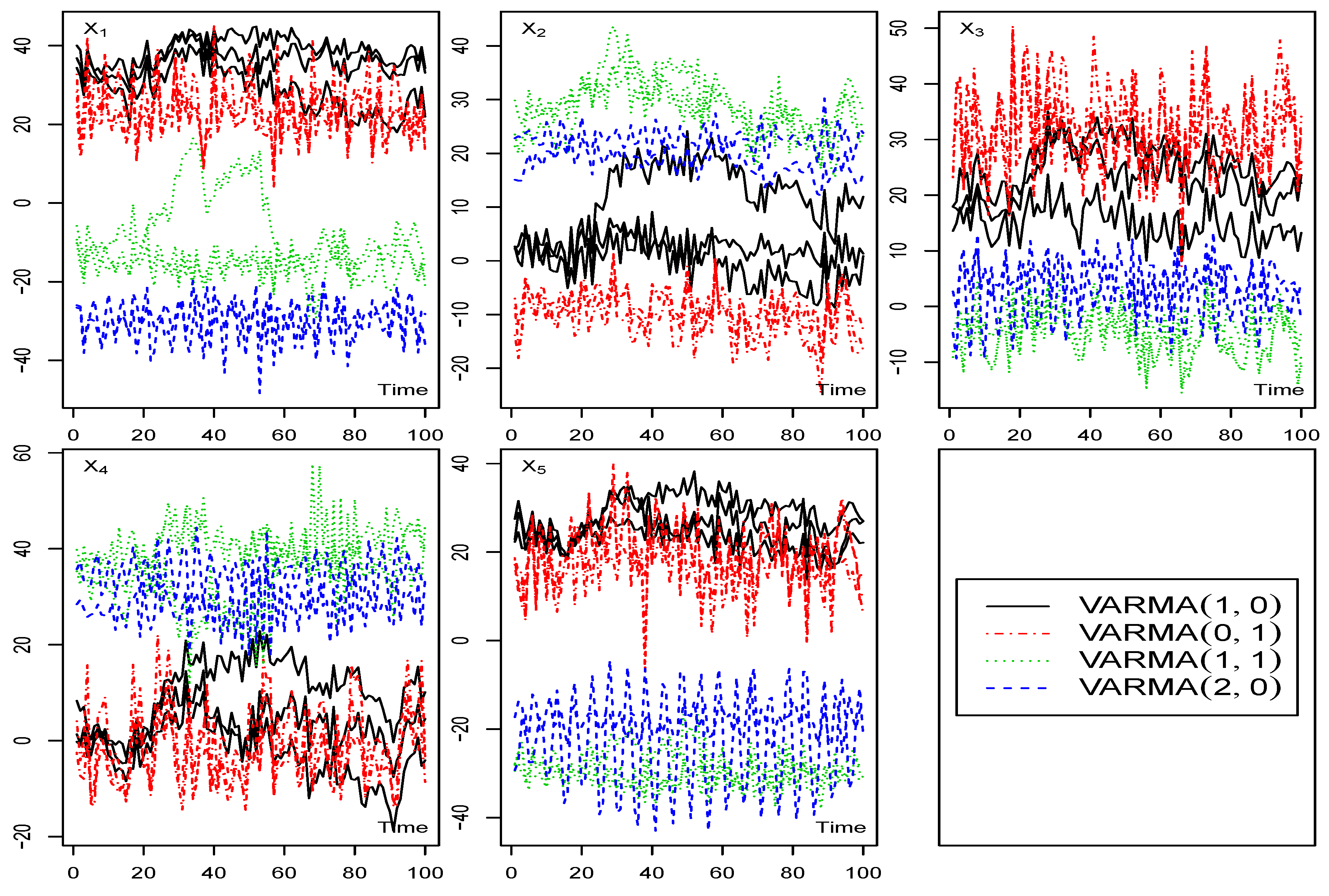
Plots of each series based on the row variables are presented in Figure 1. In these plots, the series is visually distinguished using line types and colors, which correspond to the specific model processes employed during the simulation. This coding scheme allows for clear identification and comparison of the different series within the generated data.
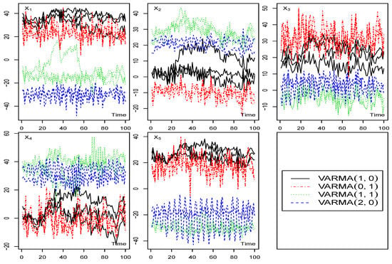
Figure 1.
The first simulated matrix time-series data: row variables by time, for all columns series.
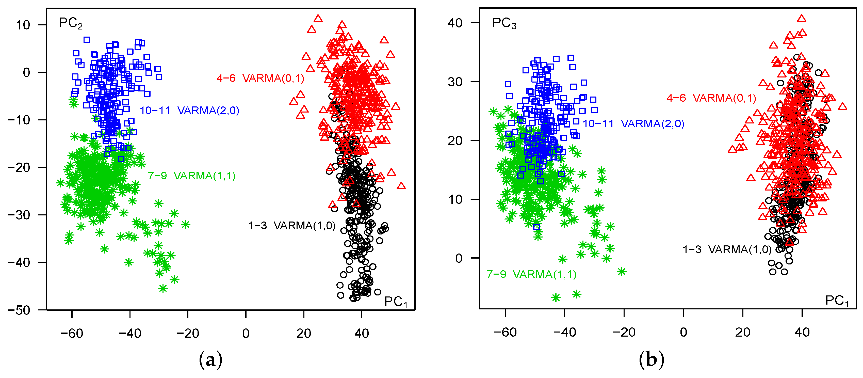
The proposed methodology was applied by first calculating the cross-autocorrelation matrices for lag based on the total variations defined in Equation (3), and then the principal components were determined over time using Equation (19). The plots of the projections of the resultant time points onto the space are shown in Figure 2a. The series are line type, color, and symbol coded according to the model process used in the simulation. The groups of time series corresponding to the different models are clearly identified. For example, column series , VARMA(1,0), in black, full lines and coded by ∘ and ‘lty=1’, column series , VARMA(0,1), in red Δ with lines (‘lty = 4’), column series , VARMA(1,1), in green ∗ with lines (‘lty = 3’), and column series , VARMA(2, 0), in blue □ with lines (‘lty = 8’). Additionally, it is evident from Figure 2 that column series exhibit noticeable differences compared to column series .
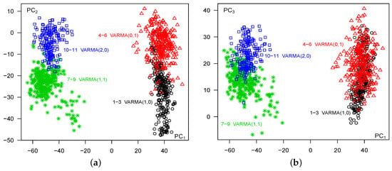
Figure 2.
The first simulated data: (a) , (b) , All Series, All Times, Lag .
These results align with the information presented in Figure 1, where the VARMA(1, 0) and VARMA(0, 1) processes appear more similar compared to the VARMA(1, 1) and VARMA(2, 0) processes, with the latter two also exhibiting some degree of similarity. Furthermore, when comparing with the other , where , similar patterns emerge. Notably, the patterns observed in the space (depicted in Figure 2b) are particularly distinct, indicating that the first two principal components adequately capture the essential characteristics of the data.
In the second example, we provide a demonstration of the foregoing theory using another simulated dataset. This dataset comprises matrix-valued time series with a dimension of and exhibits more complex structures. Similar to the first example, the dataset consists of four distinct classes () denoted as . Each class is characterized by a matrix-valued time series of dimension , , with . To generate the dataset, we employ the vec(·) operation to convert the matrix-variate series into vector variables for each class of series. Particularly, the column series are generated by a classical VAR(1) model, while the column series are generated by a threshold VAR process of order one, denoted as TVAR() (refer to Equation (30)). Furthermore, the column series are generated by a vector error correction model (VECM) process with (refer to Equation (31)) and are labeled as VECM1. Additionally, the column series are also generated using a VECM process but with a different structure ( in Equation (31)), and are labeled as VECM2. The key question we seek to address is whether the proposed methodology can effectively separate and cluster the series based solely on the available data for these S column time series.
The TVAR() model describes a q-dimensional time series process according to the following equation:
where is the threshold variable and is the threshold value. Moreover, , are coefficient matrices of dimension , and . See [64] for the details.
On the other hand, the VECM process characterizes a q-dimensional time-series process as follows:
where and are coefficient matrices of dimension , and . Moreover, are generated from ∼. See [65].
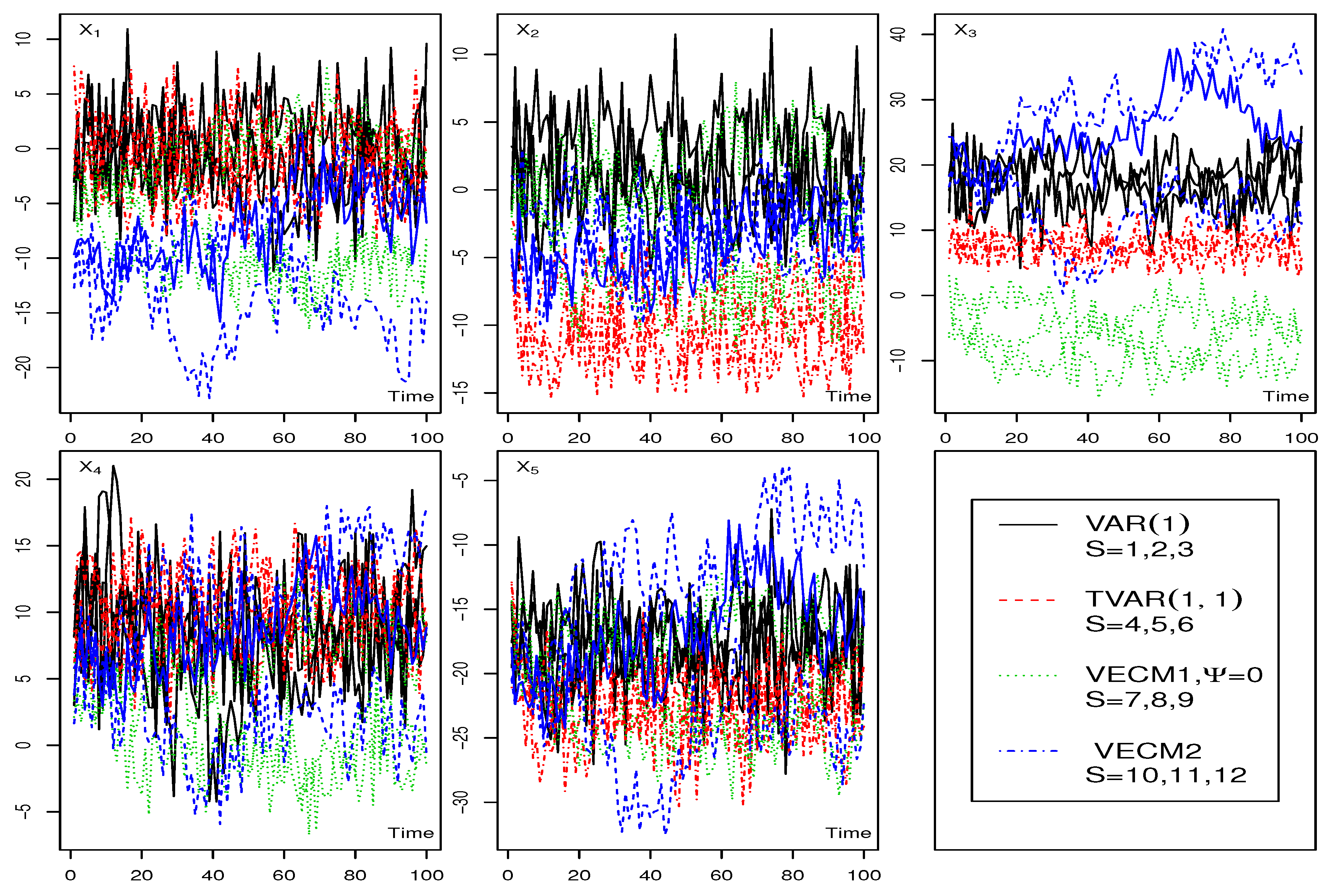
Figure 3 displays the plot of all column series by the row variables. The series are differentiated by line type, color, and symbol, indicating the model process used in the simulation. The black solid lines (‘lty = 1’) represent column series s = 1–3 generated by the VAR(1) model, the red dashed lines (‘lty = 4’) correspond to column series s = 4–6, generated by the TVAR() model, the green dotted lines (‘lty = 3’) represent column series s = 7–9, generated by the VECM1 model, and finally the blue dot-dash-dot lines (‘lty = 8’) depict the column series s = 10–12, generated by the VECM2 model. Based solely on these plots, it is evident that classifying all four groups of series is not possible. For instance, when focusing on the plots based on the row variable in Figure 3, only the column series with the blue colors appear distinct from the others. Similarly, for the plots based on , the red series seems different from the remaining series. Although there is a better sense of differentiation between the column series with different colors when observing the plots based on , there is still some overlap between the blue, black, and red series. Furthermore, there are no discernible clues for distinguishing different series when considering the plots based on and . However, our proposed PCA methodology successfully classifies all four types of series into distinct clusters as demonstrated in Figure 4.
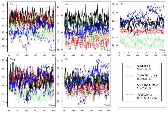
Figure 3.
The second simulated matrix time-series data: row variables by time, for all columns series.
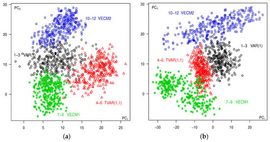
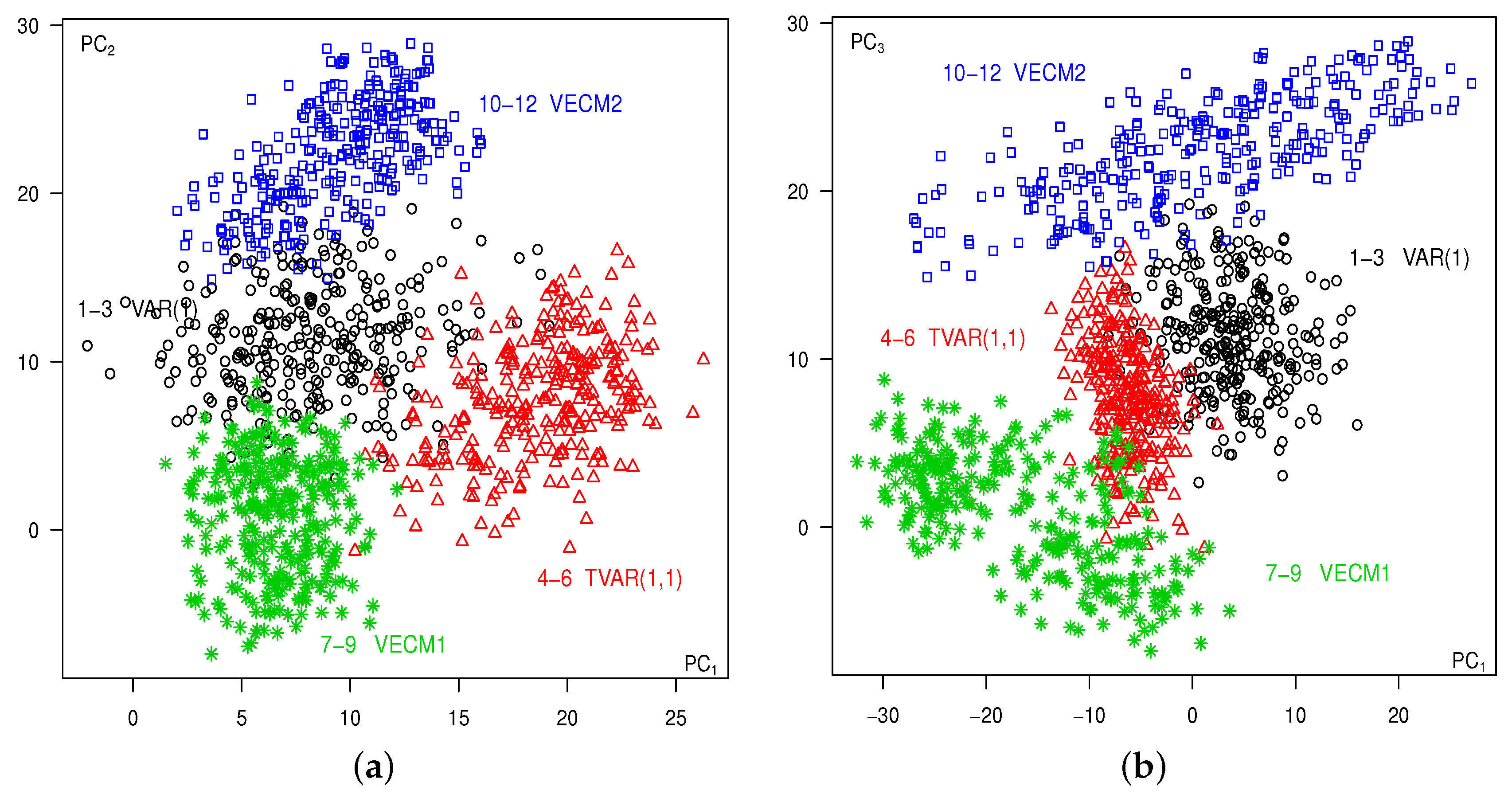
Figure 4.
The second simulated data: (a) , (b) , All Series, All Times, Lag .
The methodology involves calculating the cross-autocorrelation matrices for lag based on the total variations of Equation (3) and then deriving the principal components over time using Equation (19). Figure 4a displays the projections of the resulting time points onto the space, color-coded identically to the time series depicted in Figure 3. Groups of time series corresponding to the different models are clearly identified. Additionally, Figure 4b presents the corresponding plots projected onto the space, further highlighting the distinct clusters of the different series.
Table 1 presents a summary of the total and within variations at lag one for the second simulated data. Specifically, Table 1a displays the eigenvalues along with the percentage of variation explained by each principal component , as well as the cumulative variation percentage of the simulated data. From the table, we observe that the first two principal components account for 73.6% of the total variation, while the first three components explain 91.8% of the total variation. It is worth noting that the sum of the equals 4.64, which is less than the dimensionality J = 5. This is due to the calculation of the cross-autocorrelation matrix using lagged values.

Table 1.
Second simulated data—eigenvalues and percent variations.
In both examples, data were simulated for time series of length . Similar results were obtained for and (plots not shown), which further validate the robustness of the methodology across varying time series lengths. The consistency of the results across different lengths confirms the applicability of the methodology for both short-term and long-term time-series analysis.
5. Illustration
5.1. Auslan Sign Language Data
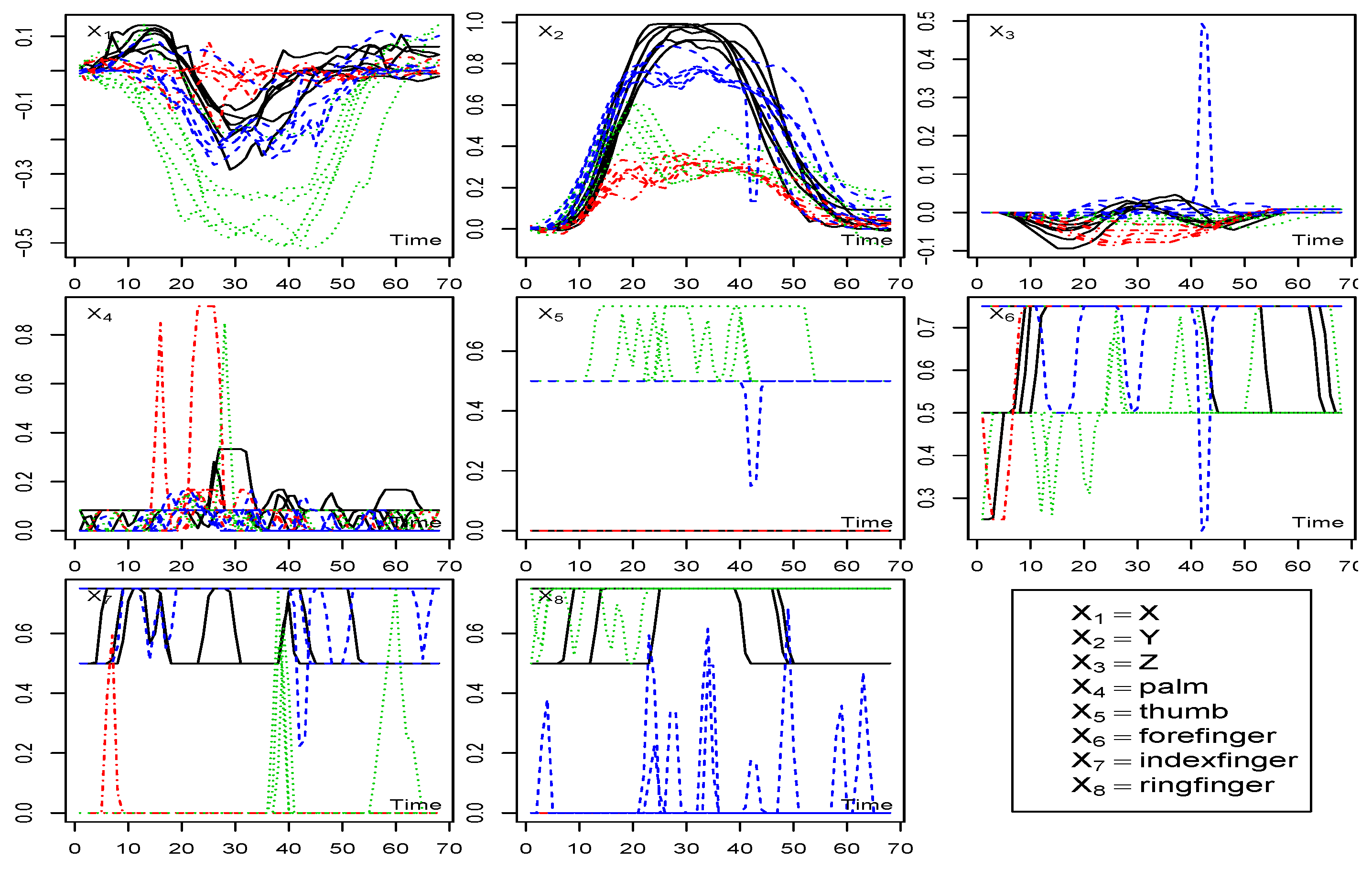
The methodology is applied to a matrix-valued time-series dataset capturing Auslan (Australian Sign Language) gestures. The dataset consists of measurements recorded from a fitted glove (representing the row variables), as different words are signed (representing column variables). The complete dataset, including additional words, series, and variables not utilized in our analysis, can be accessed on the webpage (https://archive.ics.uci.edu/ml/datasets/Australian+Sign+Language+signs, accessed on 20 April 2023) or from the UCI KDD Archive. Our analysis focuses on matrix-valued time series of dimension and of length . The row variables include , (signed in sign language in three-dimensional space ()), index finger bend, ring finger bend (with the bends in going from straight to fully bent), for four different words (): know (where indicated in relevant figures, this word is represented by the symbol black ∘ and full line (‘lty = 1’) ), maybe (red Δ and line (‘lty = 4’)) shop (green ∗ and line (‘lty = 3’)), and yes (blue □ and line (‘lty = 8’)). Each word was spoken once by each of the six “speakers”, resulting in a total of column time series, see Figure 5.

Figure 5.
Auslan data: by Time, All Series.
The objective of our analysis was to explore whether different speakers exhibited similar expressions for a given word. For instance, we investigated if there were similarities in the gestures used by different speakers when saying the word “shop”, as depicted by the green set of six series in the lower-right portion of Figure 6. Conversely, we also examined instances where there were noticeable differences across speakers, which could pose challenges for comprehending the intended meaning of the gestures. The application of the proposed row-wise matrix PCA approach is suitable for addressing these research objectives. More complete descriptive details of the variables and the experiment can be found in [66,67].
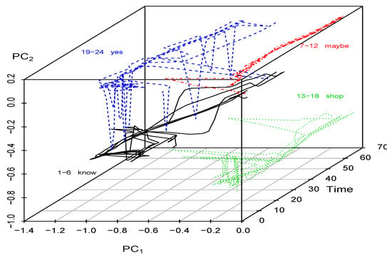
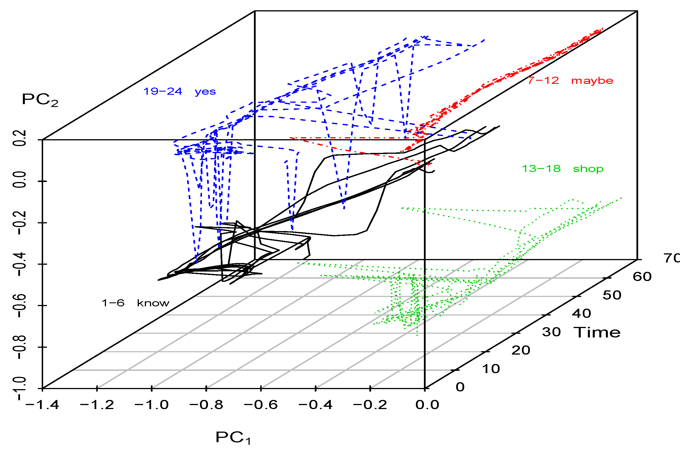
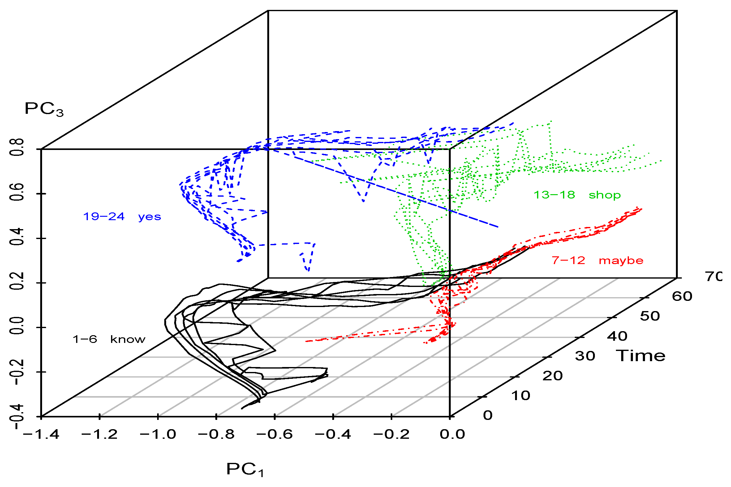
Figure 6.
Auslan data: over Time, All Series, Lag (based on total variations).
Figure 5 presents plots of each variable over time, with the color-coded representation indicating the word spoken. A quick examination reveals potential differences and noticeable variations across the series as the spoken word changes. Specifically, the plots for and , which represent the glove position in the plane, exhibit discernible differences. Conversely, certain features, such as and , demonstrate similar behaviors for the same word, while others, such as , exhibit dissimilar patterns, even for the same word. In addition, we observe that some variables, including , and , exhibit the presence of outlier values. However, the subsequent analysis conducted in Section 5.2 reveals that these specific variables do not significantly contribute to the principal component results, thereby minimizing their impact on the overall findings.
Our analysis delved into the similarities and differences in gesture expressions among speakers in Auslan using the row-wise PCA approach of the matrix-valued time-series data. By applying the proposed methodology, we aimed to gain insights into the patterns and variations in sign language gestures, contributing to a better understanding of communication dynamics in sign language contexts.
5.2. Analysis Based on Total Variations
Consider first the principal component analysis, which uses the cross-autocorrelation matrix at lag k, incorporating the cross-autocovariance based on the total variations given in Equation (3). Since corresponds to no lag-time dependencies, in this analysis, we specifically focus on the first-order time dependence, where . The resulting row cross-autocorrelation matrix, denoted as , is presented in Table 2. It is important to note that, unlike the case when , the matrix does not contain 1’s along the diagonal. This absence of 1’s in the diagonal stems from the fact that these represent lagged cross-autocorrelations.

Table 2.
Auslan data—cross-autocorrelations—.
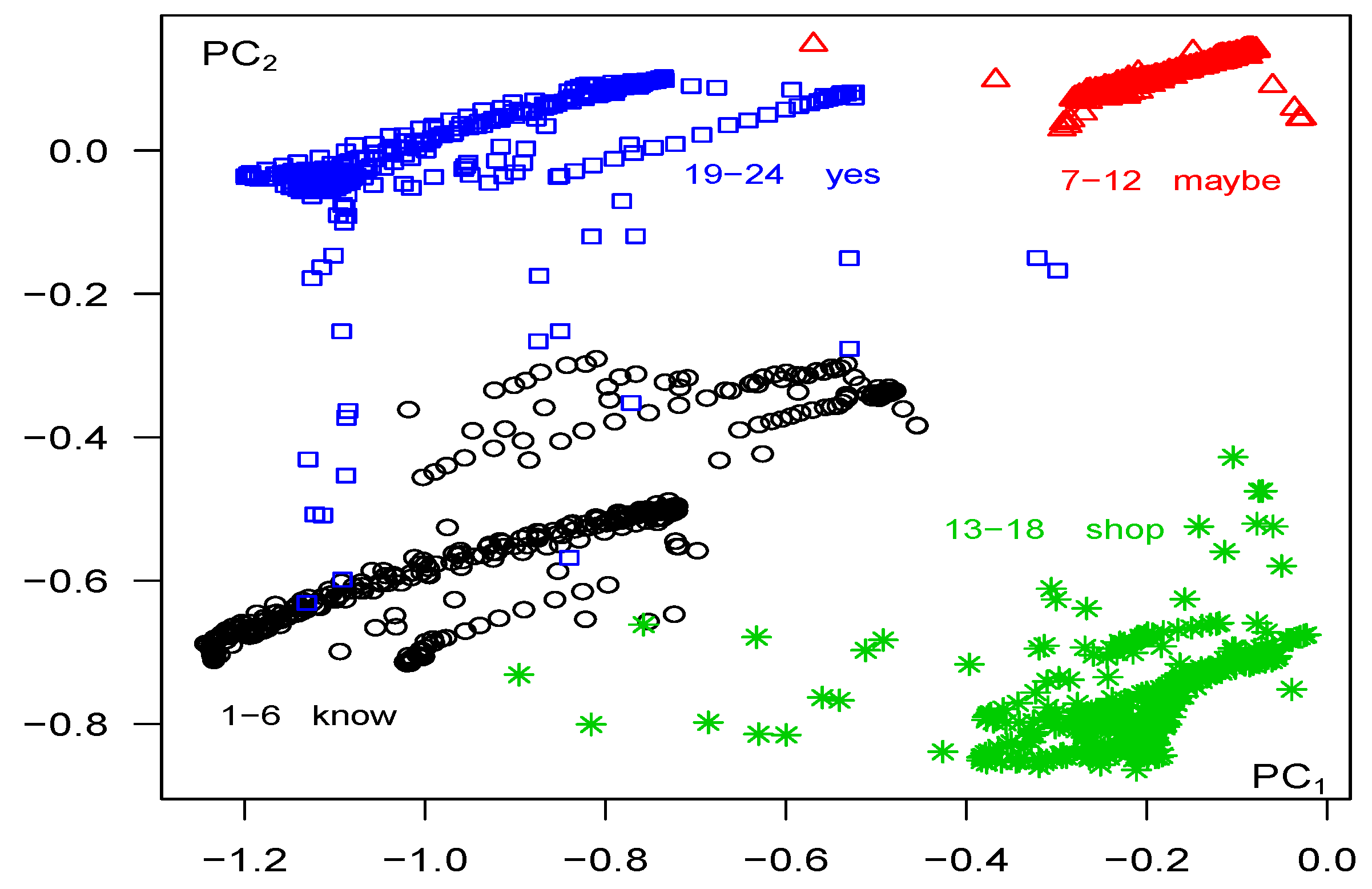
By calculating the eigenvectors of and substituting them into Equation (19), we obtain the principal components , for each column series , evaluated at each time . Figure 6 displays a plot of the first and second principal components over time, revealing the temporal dependencies. However, these plots partially obscure the underlying patterns. To provide a clearer view of the distinct patterns between series, Figure 7 depicts the first and second principal components for all series and times in a 2-dimensional plane, disregarding the time dimension. This projection effectively highlights the unique patterns present in the principal component time series, revealing both the differences and similarities across the series.
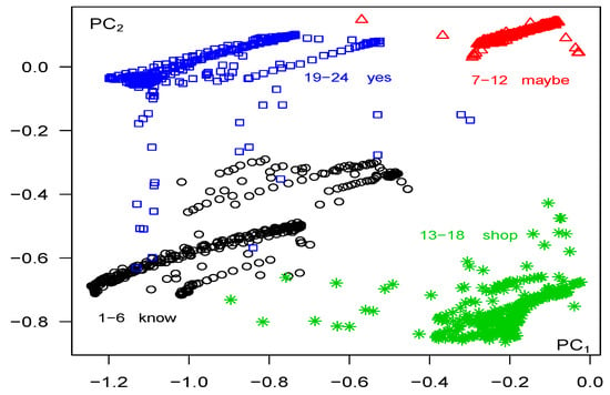
Figure 7.
Auslan data: , All Series, All Times, Lag (based on total variations).
The first observation from these plots is that all six speakers tend to produce similar patterns for a given word, indicating coherence in the results. Therefore, we conclude that series associated with the same word represent consistent speech movements. Furthermore, certain words tend to follow similar patterns. As depicted in Figure 6 and Figure 7, there is some overlap between the patterns of “know” and “yes”. On the other hand, the patterns of “shop” and “maybe” exhibit distinct characteristics.
Table 3a gives the eigenvalues together with the percent of that variation explained by each principal component , and the cumulative variation percentage. Therefore, we see that 78.6% of the variation is explained by the first four principal components, and 86.4% by the first five. Here, since the cross-autocorrelation matrix is calculated using lagged values.

Table 3.
Auslan data—eigenvalues and percent variations.
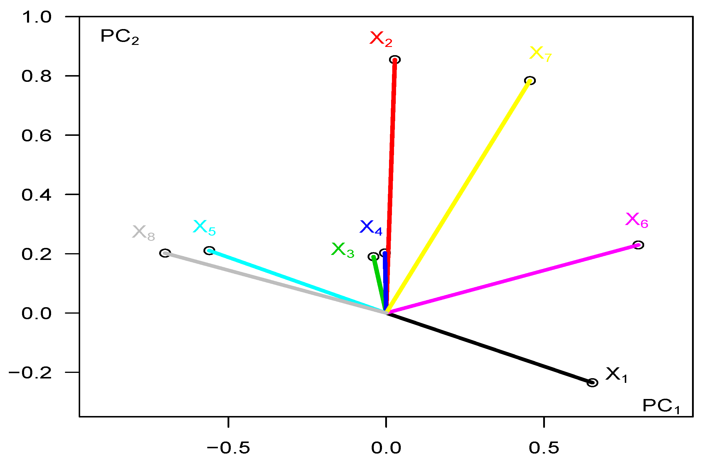
The Pearson correlation functions between the variable , and the principal component , based on the Pearson product moments given in Equation (22) are shown in Table 4a. The corresponding correlations circle, for , is plotted in Figure 8. From these values, we see that the variables and (with correlations 0.799, 0.653, and −0.700, respectively) contribute the most to the values, while the variables , and (with correlations 0.028, −0.040 and −0.004, respectively) contribute barely. That is, the position of the hand in the X-axis in space () and the amount of bend in the first two fingers (fore- and ring-fingers) are important variables. It is the variable (the Y-position in space) that dominates the values of with a correlation coefficient of 0.855. Notice that the Z-position in space () is not at all important (except marginally for the sixth principal component); likewise, the variable (palm roll) contributes very little except for its contribution to the third principal component. Collectively, it is the hand position in the X-Y plane in space and the movement of the forefinger () and the ring finger () that are the most important variables.

Table 4.
Auslan data—correlations for lag —using total variations.
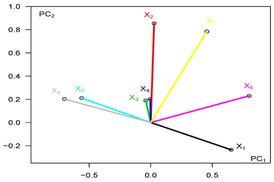
Figure 8.
Auslan data: Pearson circle for x , .
The Moran correlations calculated from Equation (26) are shown in Table 4b; the so-called loadings-based dependence measures calculated from Equation (29) are in Table 4c. Comparisons with Pearson’s correlations show that the four variables () are the most important determining factors. In addition, the variable is strongly positive with the second principal component for all three measures.
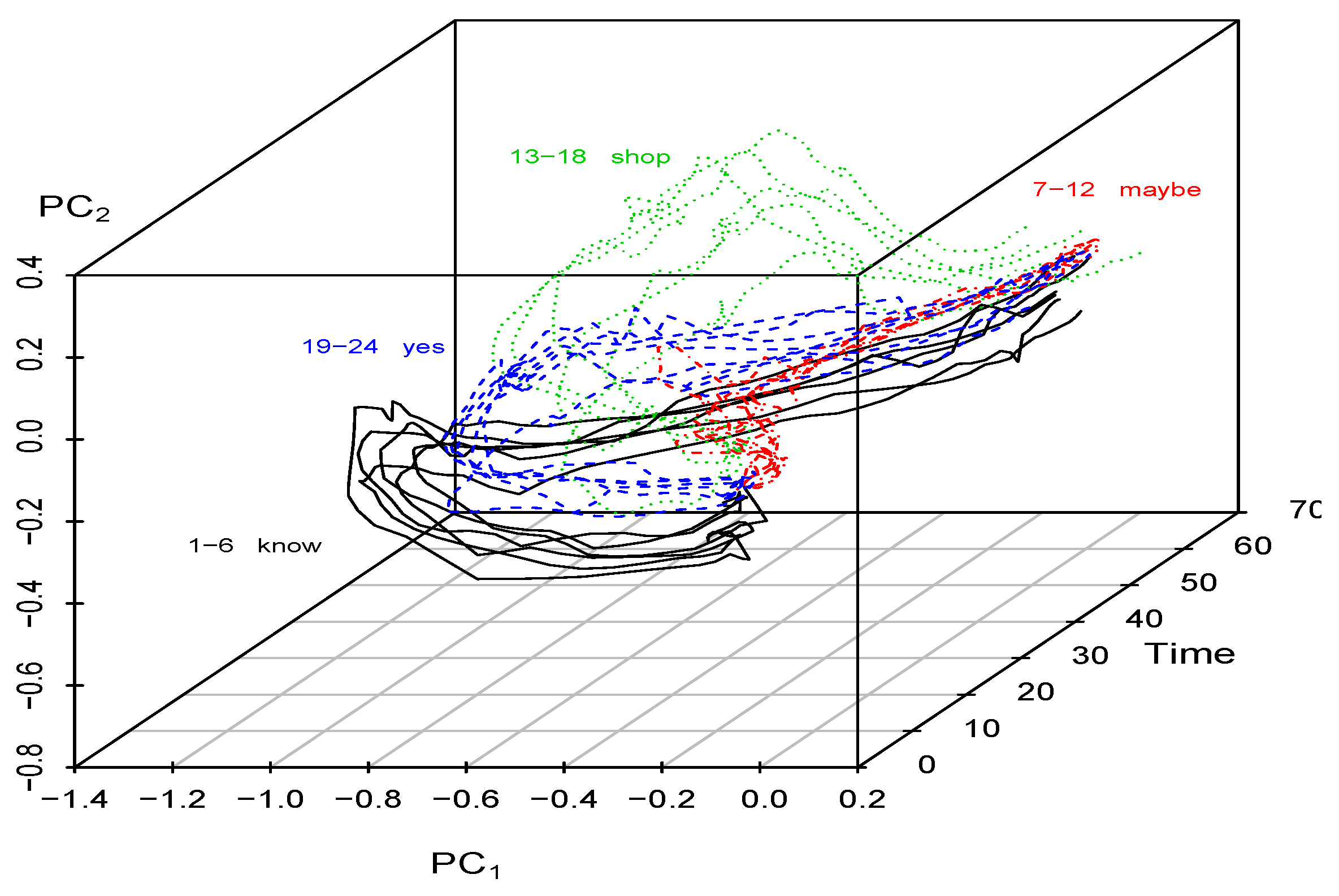
Finally, plots of by over time, for , can also be executed. These provide no further substantial information than those discussed thus far for , with one exception. The exception is the plot of versus against time, shown in Figure 9. A feature of this plot is the separation of all four words. In particular, the words “know” and “yes” no longer have overlapping patterns but are well separated. Further, we note from Table 4 that the principal component is relatively highly correlated with the variables = roll of the palm and = thumb bend for all three correlation functions. From the and plots in Figure 4, we observe that these values do not vary very much within each series but that the series for “know” and “yes” are distinct (especially for , being at the top and bottom of the plots, respectively). However, since explained only 16.8% of the overall variation (see Table 3a), too much importance should not be placed on this; rather it is an artifact of the nature of the role played by the roll of the palm and thumb bend in this particular dataset. Nevertheless, distinctions between all four words are in fact revealed by all these three principal components.
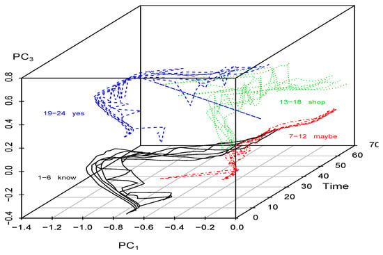
Figure 9.
Auslan data: × by Time, (based on total variations).
5.3. Within Variations and
5.3.1. Principal Components Based on within Variations
Results can be obtained for principal components when using the cross-autocorrelations based on the within variations of Equation (7). Again, take lag . The resulting eigenvalues are shown in Table 3b, along with the percent overall variation explained by a given principal component and the corresponding cumulative percent variation. Thus, the first four and first five principal components explain 70.5% and 79.9% of the variation, respectively; these are lower than the respective 78.6% and 86.4% obtained for the analysis based on the total variations. Additionally, we observe that , which is less than the value obtained when all the variations were used in the analysis. These lower variations simply reflect the fact that not all the variations in the data are being used, whereas all this information is used in the total variation results.
Since the eigenvalues differ, so do the principal component values differ from those discussed in Section 5.2. The plots of the first two principal components over time can be determined and are shown in Figure 10, while the projection onto the plane is shown in Figure 11; these can be compared with Figure 6 and Figure 7, respectively. In this case, we observe that the word “maybe” stands alone, as before. The other three words are similar to each other relative to but differ relative to . However, when compared with Figure 6 and Figure 7 based on total variations, the word patterns are not as sharply defined. This highlights the importance of an analysis based on the total variations rather than one on the within variations alone, which are just partial variations.
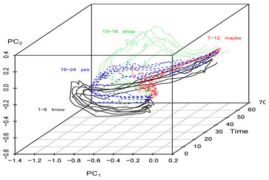
Figure 10.
Auslan data: over Time, All Series, (based on within variations).
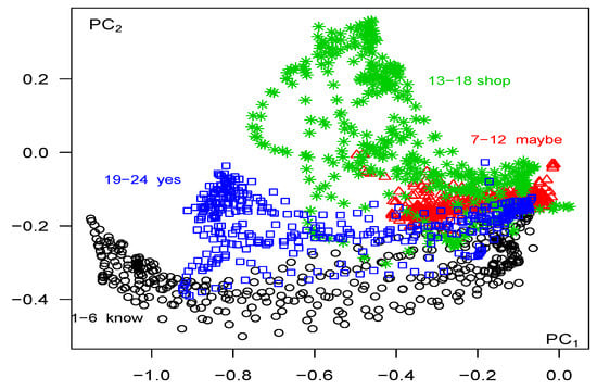
Figure 11.
Auslan data: , All Series, All Times, (based on within variations).
The correlations between principal components and variables for the analysis based on the within variations are shown in Table 5. In this case, we observe that it is the variable (and to a lesser extent, ) that is highly correlated with the first principal component . Recall, from Table 4 and the discussion in Section 5.2, that this variable has little impact on but considerable influence on when using the total variations. The within variations for correlations suggest that either or , depending on the type of correlation circle considered (see Table 5), have some influence, though the results are not overly strong.

Table 5.
Correlations for lag —using within variations.
In general, the within-variation results provide a different perspective, as they do not utilize all the variations present in the data. Consequently, these results are not as conclusive as those based on the total variations inherent in the data. However, they still offer valuable additional insights. In the case of these data, the within-variation analysis confirms the importance of as a significant variable. This finding supports the overall conclusion that the variables , and play the most crucial role in determining the separation of the spoken words, while the other variables are comparatively less pertinent.
5.3.2. Lag
By changing the lag values from to and beyond, the eigenvalues of the corresponding cross-autocorrelation matrices exhibit varying magnitudes, both for total and within variation matrices. As k increases, the cumulative variation explained by the resulting principal components also increases more rapidly. For example, the first five principal components based on the total variations of Equation (3) accounted for 86.07%, 86.43%, 87.40%, and 89.27% for respectively, of the overall variation; those based on the within variations of Equation (7) accounted for 79.17%, 79.88%, 82.92% and 85.42% for respectively. The overall variance decreased as k increased, with taking values , , , and when using total variations, for respectively.
Therefore, the actual values of the principal components varied over time for different values of k. Nevertheless, the fundamental patterns observed in the analysis of results based on the total variations and (Section 5.2) remained consistent. If higher values of k had produced different clusterings, say , it would have indicated that the time series had second-order time dependencies, which must be an essential aspect of any analysis.
6. Conclusions
In this study, we focused on exploring and uncovering the underlying structure of matrix-valued time-series data. Specifically, we extended the use of standard variance–covariance matrices for non-time-series data in principal component analyses to cross-autocorrelation matrices at time lags. , for matrix time series. This extension allowed us to capture the time dependencies present in matrix-valued time-series data by utilizing cross-autocorrelation functions. We introduced row-wise and column-wise methodologies that utilize cross-autocorrelation functions to retain the time dependencies inherent in time-series data. These methods are particularly valuable when the objective is to cluster the column or row variables of a matrix time series. By employing these methodologies, we obtained principal component time series, enabling us to visualize and compare the data using principal component plots that incorporate the additional dimension of time. Our approach is non-parametric, eliminating the need for explicit hypotheses or an a priori model, such as an autoregressive model or probabilistic structure, for time-series distributions. This allows for greater flexibility and broader applicability in analyzing diverse types of time-series data.
While our focus in this work was on comparing column (or row) series using cross-autocorrelation functions at the same lag values, it is possible that some series may exhibit similarities at different lag values. For instance, column series at lag k may resemble series at lag , where . In such cases, the entities in Equation (3) can be replaced by cross-autocovariances between variable at lag k and variable at lag . This flexibility allows for further exploration and analysis of complex time-series relationships.
In summary, our findings demonstrate the efficacy of the proposed methodology in uncovering the main structure of matrix-valued time-series data. By leveraging the strengths of principal component analysis and cross-autocorrelation functions, we can gain valuable insights into the underlying patterns and relationships within complex time series data.
Author Contributions
All authors contributed equally. All authors have read and agreed to the published version of the manuscript.
Funding
This research received no external funding.
Data Availability Statement
The data that support the findings of this study are available on request from the corresponding author. The data set can be found at https://archive.ics.uci.edu/ml/datasets/Australian+Sign+Language+signs (accessed on 20 April 2023).
Conflicts of Interest
The authors declare no conflict of interest.
References
- Lin, J.; Michailidis, G. Regularized estimation and testing for high-dimensional multi- block vector-autoregressive models. J. Mach. Learn. Res. 2017, 18, 4188–4236. [Google Scholar]
- Mills, T.C. The Econometric Modelling of Financial Time Series; Cambridge University Press: Cambridge, UK, 1993. [Google Scholar]
- Samadi, S.Y.; Billard, L. Analysis of dependent data aggregated into intervals. J. Multivar. Anal. 2021, 186, 104817. [Google Scholar] [CrossRef]
- Samadi, S.Y.; Herath, H.M.W.B. Reduced-rank envelope vector autoregressive models. 2023; preprint. [Google Scholar]
- Seth, A.K.; Barrett, A.B.; Barnett, L. Granger causality analysis in neuroscience and neuroimaging. J. Neurosci. 2015, 35, 3293–3297. [Google Scholar] [CrossRef] [PubMed]
- Zhou, H.; Li, L.; Zhu, H. Tensor regression with applications in neuroimaging data analysis. J. Am. Stat. Assoc. 2013, 108, 540–552. [Google Scholar] [CrossRef] [PubMed]
- Liao, T.W. Clustering of time series—A survey. Pattern Recognit. 2005, 38, 1857–1874. [Google Scholar] [CrossRef]
- Košmelj, K.; Batagelj, V. Cross-sectional approach for clustering time varying data. J. Classif. 1990, 7, 99–109. [Google Scholar] [CrossRef]
- Goutte, C.; Toft, P.; Rostrup, E. On clustering fMRI time series. Neuroimage 1999, 9, 298–310. [Google Scholar] [CrossRef] [PubMed]
- Policker, S.; Geva, A.B. Nonstationary time series analysis by temporal clustering. IEEE Trans. Syst. Man Cybernet-B Cybernet 2000, 30, 339–343. [Google Scholar] [CrossRef]
- Prekopcsák, Z.; Lemire, D. Time series classification by class-specific Mahalanobis distance measures. Adv. Data Anal. Classif. 2012, 6, 185–200. [Google Scholar]
- Harrison, L.; Penny, W.D.; Friston, K. Multivariate autoregressive modeling of fMRI time series. Neuroimage 2003, 19, 1477–1491. [Google Scholar] [CrossRef]
- Maharaj, E.A. Clusters of time series. J. Classif. 2000, 17, 297–314. [Google Scholar] [CrossRef]
- Piccolo, D. A distance measure for classifying ARIMA models. J. Time Ser. Anal. 1990, 11, 153–164. [Google Scholar] [CrossRef]
- Alonso, A.M.; Berrendero, J.R.; Hernández, A.; Justel, A. Time series clustering based on forecast densities. Comput. Stat. Data Anal. 2006, 51, 762–776. [Google Scholar] [CrossRef]
- Vilar, J.A.; Alonso, A.M.; Vilar, J.M. Non-linear time series clustering based on non-parametric forecast densities. Comput. Stat. Data Anal. 2010, 54, 2850–2865. [Google Scholar] [CrossRef]
- Owsley, L.M.D.; Atlas, L.E.; Bernard, G.D. Self-organizing feature maps and hidden Markov models for machine-tool monitoring. IEEE Trans. Signal Process. 1997, 45, 2787–2798. [Google Scholar] [CrossRef]
- Douzal-Chouakria, A.; Nagabhushan, P. Adaptive dissimilarity index for measuring time series proximity. Adv. Data Anal. Classif. 2007, 1, 5–21. [Google Scholar] [CrossRef]
- Jeong, Y.; Jeong, M.; Omitaomu, O. Weighted dynamic time warping for time series classification. Pattern Recognit. 2011, 44, 2231–2240. [Google Scholar] [CrossRef]
- Yu, D.; Yu, X.; Hu, Q.; Liu, J.; Wu, A. Dynamic time warping constraint learning for large margin nearest neighbor classification. Inf. Sci. 2011, 181, 2787–2796. [Google Scholar] [CrossRef]
- Liao, T.W. A clustering procedure for exploratory mining of vector time series. Pattern Recognit. 2007, 40, 2550–2562. [Google Scholar] [CrossRef]
- Košmelj, K.; Zabkar, V. A methodology for identifying time-trend patterns: An application to the advertising expenditure of 28 European countries in the 1994–2004 period. In Lecture Notes in Computer Science, KI: Advances in Artificial Inteligence; Furbach, U., Ed.; Springer: Berlin/Heidelberg, Germany, 2008; pp. 92–106. [Google Scholar]
- Kalpakis, K.; Gada, D.; Puttagunta, V. Distance measures for effective clustering of ARIMA time-series. Data Min. 2001, 1, 273–280. [Google Scholar]
- Kakizawa, Y.; Shumway, R.H.; Taniguchi, N. Discrimination and clustering for mulitvariate time series. J. Am. Stat. Assoc. 1998, 93, 328–340. [Google Scholar] [CrossRef]
- Shumway, R.H. Time-frequency clustering and discriminant analysis. Stat. Probab. Lett. 2003, 63, 307–314. [Google Scholar] [CrossRef]
- Vilar, J.M.; Vilar, J.A.; Pértega, S. Classifying time series data: A nonparametric approach. J. Classif. 2009, 26, 3–28. [Google Scholar] [CrossRef]
- Forni, M.; Hallin, M.; Lippi, M.; Reichlin, L. The generalized dynamic factor model: Identification and estimation. Rev. Econ. Stat. 2000, 82, 540–554. [Google Scholar] [CrossRef]
- Forni, M.; Lippi, M. The generalized factor model: Representation theory. Econom. Theory 2001, 17, 1113–1141. [Google Scholar] [CrossRef]
- Garcia-Escudero, L.A.; Gordaliza, A. A proposal for robust curve clustering. J. Classif. 2005, 22, 185–201. [Google Scholar] [CrossRef]
- Hebrail, G.; Hugueney, B.; Lechevallier, Y.; Rossi, F. Exploratory analysis of functional data via clustering and optimal segmentation. Neurocomputing 2010, 73, 1125–1141. [Google Scholar] [CrossRef]
- Huzurbazar, S.; Humphrey, N.F. Functional clustering of time series: An insight into length scales in subglacial water flow. Water Resour. Res. 2008, 44, W11420. [Google Scholar] [CrossRef]
- Serban, N.; Wasserman, L. CATS: Clustering after transformation and smoothing. J. Am. Stat. Assoc. 2005, 100, 990–999. [Google Scholar] [CrossRef]
- MacQueen, J.B. Some methods for classification and analysis of multivariate observations. In Proceedings of the Fifth Berkeley Symposium on Mathematical Statistics; Le Cam, L., Neyman, J., Eds.; University of California Press: Oakland, CA, USA, 1967; pp. 281–297. [Google Scholar]
- Ward, J.H. Hierarchical grouping to optimize an objective function. J. Am. Stat. Asoc. 1963, 58, 236–244. [Google Scholar] [CrossRef]
- Kaufman, L.; Rousseeuw, P.J. Finding Groups in Data: An Introduction to Cluster Analysis; Wiley: New York, NY, USA, 1990. [Google Scholar]
- Dunn, J. A fuzzy relative of the ISODATA process and its use in detecting compact, well separated clusters. J. Cybern. 1974, 3, 32–57. [Google Scholar] [CrossRef]
- Beran, J.; Mazzola, G. Visualizing the relationship between time series by hierarchical smoothing models. J. Comput. Graph. Stat. 1999, 8, 213–228. [Google Scholar]
- Wismüller, A.; Lange, O.; Dersch, D.R.; Leinsinger, G.L.; Hahn, K.; Pütz, B.; Auer, D. Cluster analysis of biomedical image time series. Int. J. Comput. Vis. 2002, 46, 103–128. [Google Scholar] [CrossRef]
- Box, G.E.P.; Jenkins, G.M.; Reinsel, G.C.; Ljung, G.M. Time Series Analysis: Forecasting and Control, 4th ed.; Holden-Day: San Francisco, CA, USA, 2015. [Google Scholar]
- Brockwell, P.J.; Davis, R.A. Time Series: Theory and Methods; Springer: New York, NY, USA, 1991. [Google Scholar]
- Park, J.H.; Samadi, S.Y. Heteroscedastic modelling via the autoregressive conditional variance subspace. Can. J. Stat. 2014, 42, 423–435. [Google Scholar] [CrossRef]
- Park, J.H.; Samadi, S.Y. Dimension Reduction for the Conditional Mean and Variance Functions in Time Series. Scand. J. Stat. 2020, 47, 134–155. [Google Scholar] [CrossRef]
- Samadi, S.Y.; Hajebi, M.; Farnoosh, R. A semiparametric approach for modelling multivariate nonlinear time series. Can. J. Stat. 2019, 47, 668–687. [Google Scholar] [CrossRef]
- Walden, A.; Serroukh, A. Wavelet Analysis of Matrix-valued Time Series. Proc. Math. Phys. Eng. Sci. 2002, 458, 157–179. [Google Scholar] [CrossRef]
- Wang, H.; West, M. Bayesian analysis of Matrix Normal Graphical Models. Biometrika 2009, 96, 821–834. [Google Scholar] [CrossRef]
- Samadi, S.Y. Matrix Time Series Analysis. Ph.D. Dissertation, University of Georgia, Athens, GA, USA, 2014. [Google Scholar]
- Samadi, S.Y.; Billard, L. Matrix time series models. 2023; preprint. [Google Scholar]
- Cryer, J.D.; Chan, K.-S. Time Series Analysis; Springer: New York, NY, USA, 2008. [Google Scholar]
- Shumway, R.H.; Stoffer, D.S. Time Series Analysis and Its Applications; Springer: New York, NY, USA, 2011. [Google Scholar]
- Whittle, P. On the fitting of multivariate autoregressions, and the approximate canonical factorization of a spectral density matrix. Biometrika 1963, 50, 129–134. [Google Scholar] [CrossRef]
- Jones, R.H. Prediction of multivariate time series. J. Appl. Meteorol. 1964, 3, 285–289. [Google Scholar] [CrossRef]
- Webb, A. Statistical Pattern Recognition; Hodder Headline Group: London, UK, 1999. [Google Scholar]
- Johnson, R.A.; Wichern, D.W. Applied Multivariate Statistical Analysis, 7th ed.; Prentice Hall: Hoboken, NJ, USA, 2007. [Google Scholar]
- Joliffe, I.T. Principal Component Analysis; Springer: New York, NY, USA, 1986. [Google Scholar]
- Anderson, T.W. An Introduction to Multivariate Statistical Analysis, 2nd ed.; John Wiley: New York, NY, USA, 1984. [Google Scholar]
- Samadi, S.Y.; Billard, L.; Meshkani, M.R.; Khodadadi, A. Canonical correlation for principal components of time series. Comput. Stat. 2017, 32, 1191–1212. [Google Scholar] [CrossRef]
- Billard, L.; Douzal-Chouakria, A.; Samadi, S.Y. An Exploratory Analysis of Multiple Multivariate Time Series. In Proceedings of the 1st International Workshop Advanced Analytics Learning on Temporal Data AALTD 2015, Porto, Portugal, 11 September 2015; Volume 3, pp. 1–8. [Google Scholar]
- Jäckel, P. Monte Carlo Methods in Finance; John Wiley: New York, NY, USA, 2002. [Google Scholar]
- Rousseeuw, P.; Molenberghs, G. Transformation of non positive semidefnite correlation matrices. Commun. Stat. Theory Methods 1993, 22, 965–984. [Google Scholar] [CrossRef]
- Cai, T.T.; Ma, Z.; Wu, Y. Sparse PCA: Optimal rates and adaptive estimation. Ann. Stat. 2013, 41, 3074–3110. [Google Scholar] [CrossRef]
- Guan, Y.; Dy, J.G. Sparse probabilistic principal component analysis. J. Mach. Learn. Res. 2009, 5, 185–192. [Google Scholar]
- Lu, M.; Huang, J.Z.; Qian, X. Sparse exponential family Principal Component Analysis. Pattern Recognit. 2016, 60, 681–691. [Google Scholar] [CrossRef] [PubMed]
- Moran, P.A.P. The interpretation of statistical maps. J. R. Stat. Soc. A 1948, 10, 243–251. [Google Scholar] [CrossRef]
- Lo, C.M.; Zivot, E. Threshold cointegration and nonlinear adjustment to the law of one price. Macroecon. Dyn. 2001, 5, 533–576. [Google Scholar] [CrossRef]
- Engle, R.F.; Granger, C.W.J. Co-integration and error correction: Representation, estimation and testing. Econometrica 1987, 55, 251–276. [Google Scholar] [CrossRef]
- Kadous, M.W. Recognition of Australian Sign Language Using Instrumented Gloves. Bachelor’s Thesis, University of South Wales, Newport, UK, 1995; 136p. [Google Scholar]
- Kadous, M.W. Learning comprehensible descriptions and multivariate time series. In Proceedings of the Sixteenth International Conference on Machine Learning, Bled, Slovenia, 27–30 June 1999; Bratko, I., Dzeroski, S., Eds.; Morgan Kaufmann Publishers: San Fransisco, CA, USA, 1999; pp. 454–463. [Google Scholar]
Disclaimer/Publisher’s Note: The statements, opinions and data contained in all publications are solely those of the individual author(s) and contributor(s) and not of MDPI and/or the editor(s). MDPI and/or the editor(s) disclaim responsibility for any injury to people or property resulting from any ideas, methods, instructions or products referred to in the content. |
© 2023 by the authors. Licensee MDPI, Basel, Switzerland. This article is an open access article distributed under the terms and conditions of the Creative Commons Attribution (CC BY) license (https://creativecommons.org/licenses/by/4.0/).

