Article

An Efficient Convolutional Neural Network with Supervised Contrastive Learning for Multi-Target DOA Estimation in Low SNR

1
School of Information Science and Engineering, Harbin Institute of Technology, Weihai 264209, China
2
School of Marine Science and Technology, Northwestern Polytechnical University, Xi’an 710072, China
3
Institute of Big Data Science and Industry, Shanxi University, Taiyuan 030006, China
*
Author to whom correspondence should be addressed.
Axioms 2023, 12(9), 862; https://doi.org/10.3390/axioms12090862
Submission received: 16 July 2023 / Revised: 23 August 2023 / Accepted: 2 September 2023 / Published: 7 September 2023
(This article belongs to the Special Issue Differential Equations and Inverse Problems)

Abstract

:
In this paper, a modified high-efficiency Convolutional Neural Network (CNN) with a novel Supervised Contrastive Learning (SCL) approach is introduced to estimate direction-of-arrival (DOA) of multiple targets in low signal-to-noise ratio (SNR) regimes with uniform linear arrays (ULA). The model is trained using an on-grid setting, and thus the problem is modeled as a multi-label classification task. Simulation results demonstrate the robustness of the proposed approach in scenarios with low SNR and a small number of snapshots. Notably, the method exhibits strong capability in detecting the number of sources while estimating their DOAs. Furthermore, compared to traditional CNN methods, our refined efficient CNN significantly reduces the number of parameters by a factor of sixteen while still achieving comparable results. The effectiveness of the proposed method is analyzed through the visualization of latent space and through the advanced theory of feature learning.

1. Introduction

Precise direction-of-arrival (DOA) estimation using an antenna or sensor array is critical in various applications, such as microphone, sonar, source localization, and radar. Numerous algorithms have been invented to tackle the DOA estimation problem, and among them, the subspace-based estimation algorithms are well known for their capacity to give a high-resolution estimation. These include MUSIC (Multiple SIgnal Classification), ESPRIT (Estimation of Signal Parameters via Rotational Invariance Techniques), Root-MUSIC (R-MUSIC) [1,2,3], homotopy method [4,5], multigrid method [6,7], and multigrid-homotopy method [8]. However, in low signal-to-noise ratio (SNR) environments, they suffer from significant biases. To address this issue, deep learning methods have been employed.
Deep learning (DL) methods have recently emerged as promising approaches for direction-of-arrival (DOA) estimation, offering significant advantages over traditional subspace and sparse methods [9,10]. For DOA estimation of multitarget in harsh environments, multi-layer perceptron (MLP) method focuses on the robustness to array imperfections [11]; however, the model is trained at each individual SNR and fixed on a two-source target. The deep Convolutional Neural Networks (CNN) have achieved superior on-grid accuracy in low SNR regimes where the number of sources is unknown, but obtained a relatively large fully connected layer size and increased the number of parameters [12]. The authors in [13] leverage the eigenvalues from Full-row Toeplitz Matrices Reconstruction (FTMR) to enumerate the number of sources, but the error rate is still around 10% at −10 dB. Another approach proposed in [14] is a grid-less method that exploits the Toeplitz property and does not suffer from grid mismatch, but its performance is not sufficient in limited source numeration.
This paper proposes the CNN with Supervised Contrastive Learning (CNN-SCL) for multi-target DOA estimation in low SNR regimes, which is combined with Supervised Contrastive Learning (SCL) for pretraining. SCL is an extension of contrastive learning [15] in supervised task, which encourages the clustering of similar examples in the latent space while promoting the separation of different samples [16]. In this work, SCL is introduced to improve the performance of the model in detecting the number of sources and their DOAs, while also enabling the use of fewer parameters compared to prior work [12]. We make both our demo page and source-code publicly available in https://github.com/Meur3ault/Contrastive-Learning-for-Low-SNR-DOA on 12 September 2023.

2. Signal Model and Data Setting

This study focuses on the following scenario: K far-field and narrowband signals s(t) impinge on an array of antennas from direction angle θ = θ 1 , θ 2 , θ 3 , θ k with L antennas placed uniformly linear in spacing of d. Signals received at the l th sensor is given by:
y l t = k = 1 K s k t e j 2 π λ l 1 d sin θ k + n l t
where 1 l L and n l t is the additive white noise at l th sensors. They can be conveniently expressed in the following matrix form:
y t = y 1 t , y 2 t , , y L t T = a θ 1 , a θ 2 , , a θ K s t + n t = A s t + n t  
and where s ( t ) , y ( t ) , n ( t ) are the transmit signal vector, received signal vector, and noise vector, respectively. Moreover, a ( θ ) , denotes a steering vector represented as:
a θ k = e j 2 π λ 0 d sin θ k e j 2 π λ 1 d sin θ k e j 2 π λ L 1 d sin θ k = e j ω 0 τ 1 i e j ω 0 τ 21 e j ω 0 τ L i
that represents the phases of i th transmit signal in L sensors. The w 0 is angular frequency of transmit signal and τ l i is the delay of i th signal at l th sensor or antenna. The matrix A or A θ is L × K array manifold matrix with steering vectors in columns. The ideal array covariance matrix or spatial covariance is given by:
R y = E y t y H t = A θ R s A H θ + σ 2 I L
where E [ ] and ( ) H denote the expectation and conjugate transpose. In addition, noises are regarded as circularly-symmetric Gaussian white noises with the same variance independent of each other, while noise covariance matrix σ 2 I L is with diagonal elements only. The R s = E s ( t ) s H ( t ) represents signal covariance matrix with zero means. R y is the array received signal covariance matrix or spatial covariance matrix, which is complex and Hermitian. In practice, the ideal matrix is unknown and usually substituted by its T -snapshots unbiased estimation R ~ y = 1 T t = 1 T y ( t ) y H ( t ) . Here the model is trained with both sample R ~ y and ideal R y . The input data X (generated by R y ) and X ~ (generated by R ~ y ) in proposed model CNN-SCL are L × L × 3 matrices, containing the real part, imaginary part, and phase of the spatial covariance matrices, i.e., X : , : , 1 = R e R y , X : , : , 2 = I m R y , and X : , : , 3 = R y . During both the pretraining and training phases, the generated data X ( i ) is obtained by selecting the discretized angles across the range 60 , , 1 , 0 , 1 , , 60 with 121 grids. The label set H contains the i th label H ( i ) for data X ( i ) , which is sum one-hot 121 × 1 vector of multiple or single discretized angles with respect to X ( i ) , e.g., the data X ( i ) generated by {−60°, −59°, 60°} angles corresponds to 121 × 1 vector H ( i ) = [ 1,1 , 0 , , 1 ] T . Thus, the data set is D = X ( 1 ) , H ( 1 ) , X ( 2 ) , H ( 2 ) , , X ( N ) , H ( N )   of   size   N . In this paper, the inter-element distance d is set to half the wavelength ( d = λ / 2 ) and the number of array elements L is 16.

3. The Proposed Model

The layout of our proposed model is depicted in Figure 1, in which the backbone is modified upon the conventional convolutional structure [17]. The model comprises two distinct components: a feature extractor, denoted as f, consisting of four convolutional layers, and a classifier, denoted as g, consisting of six fully connected (FC) layers. The first four FC layers of the classifier have their weights shared to enhance generalization and reduce the number of parameters [18]. The proposed model is trained in two stages, namely pretraining and training. The total number of learnable parameters in our model is 1,740,457, which is significantly less than the 28.2 million in the current CNN model [12].

3.1. Pretraining Stage

In the pretraining phase, where SCL is applied, we built up a data set including single-source data in both ideal data X   and sampled X ~ of T snapshot. As data augmentation increases the amount of training data to avoid overfitting, the sampled version X ~ are considered as the augmentation of X   , i.e., X are generated directly from equation (4), w h i l e   X ~   i s   u n b i a s e d e s t i m a t i o n v e r s i o n . The purpose of data augmentation is to impose consistency regularization, which encourages the model to produce the same classification even when inputs are perturbed [19]. The inclusion of uncertainty in X ~ makes it a suitable option for this purpose. After inputs are fed into the feature extractor f , the features Z = f X and Z ~ = f X ~ are generated in latent space. To achieved better robustness and stability in harsh environments, the supervised contrastive loss is introduced [16], namely supervised contrastive learning objective, denoted by:
L s u p = i I log 1 P i p P i exp Z i Z p / τ a A i e x p Z i Z a / τ
where i I ≡ {1 ... 2N} is the index of an arbitrary sample in data set combined X ~ and X   , A i I i , and τ ∈ R+ is a scalar temperature parameter. P i = p A i : H p = H i is the set of indices of all other samples that are same class with i th sample (and thus in equation (5), the Z ~ and Z are indiscriminately denoted as Z cause indexes already involve both). | P ( i ) | is its cardinality. The supervised contrastive loss encourages the clustering of similar examples in the latent space while also promoting the separation of different samples 16. In pretraining, all the data are single-source and so are the labels, which are one-hot among 60 , , 1 , 0 , 1 , , 60 . Pretraining can be regarded as a supervised contrastive learning process involving 121 classes. The size of the output feature is 32 × 32. For convenience, we dispatched Z ( i ) or Z ~ ( i ) into length 32 with 32 views in contrastive training [20].
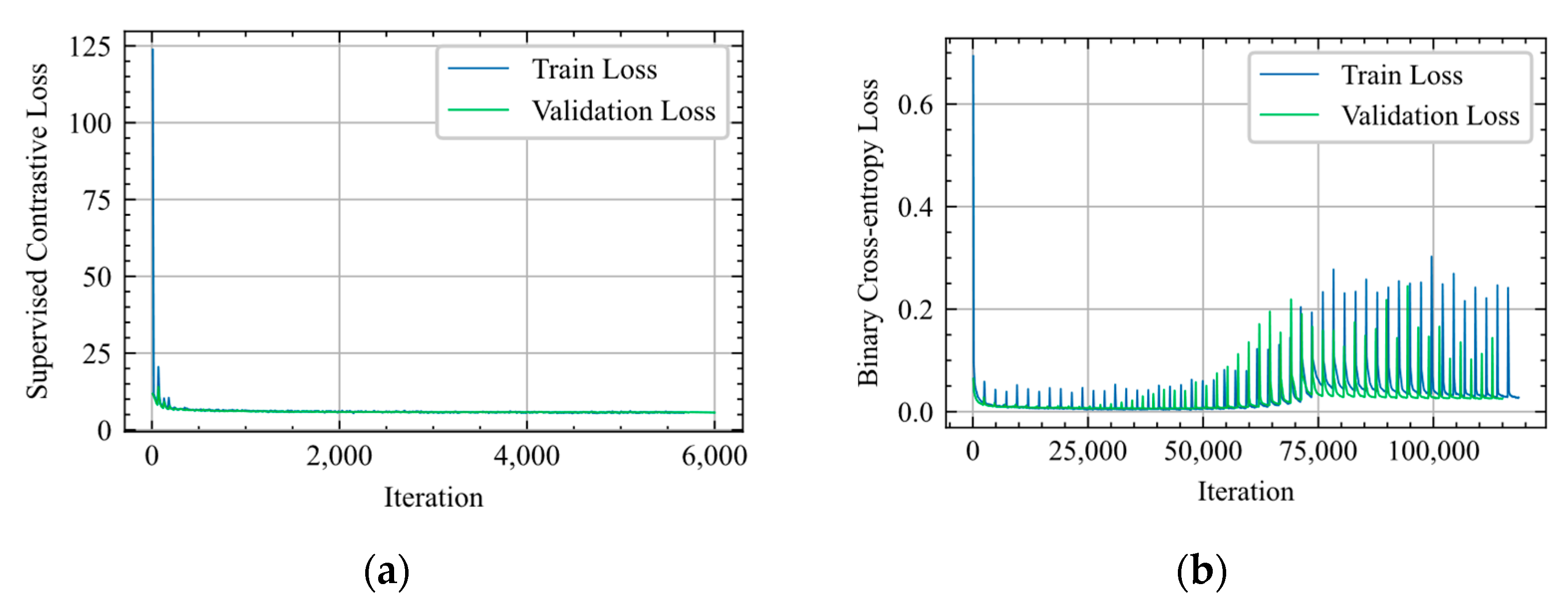
To generate data, consider K = 1 and generate on-grid data and label in low SNRs among {−15, −10, −5, 0} dB. The number of angle pairs of ideal X is 121 1 × 4 = 484 so as X ~ , leading to a double size of data set to D 0 = 484 × 2, where X ~ is the unbiased estimation of X with 100 snapshots. To increase the diversity of data pairs in each randomly split batch, we generated the data set D 0 ten times, resulting in a final data set size of D = 484 × 2 × 10 = 9680. The data set was randomly split into a validation set (10%) and a training set (90%) with a batch size of 130. The feature extractor was trained for 100 epochs using Adam optimization [21] with an initial learning rate of 0.001, β1 = 0.9, and β2 = 0.999. To achieve convergence, the learning rate was decayed by a factor of 1/ 2 every 10 epochs, and the model was saved when the validation loss reached its minimum. The loss curve is shown in Figure 2a, with a minimum loss of 5.5927.

3.2. Training Stage

In the training phase after pretraining, the feature extractor would be trained with initialized classifier together. The final layer in classifier is sigmoid to retain the value in [0, 1] through 121 × 1 output vector H ^ i :
H ^ i = g f X ~ i   = p ^ 60 p ^ 60
The value p ^ i indicates the probability spectrum of incident signals with on-grid angles. The sigmoid function allows for the prediction of multiple sources and enables the model to handle data beyond that of a single source, thereby input X ~   differs from the pretraining stage. In the training stage, the X ~ are sampled version inputs, as with those in pretraining. Instead of a single source, X ~ here were generated from multiple sources. Finally, the loss L T for training is:
L T = 1 N i = 1 N L H ^ i ; H i
while L is the binary cross-entropy loss:
L H ^ i ; H i = 1 121 n = 1 121 H i n l o g H ^ i n + 1 H i n l o g 1 H ^ i n  
For the input in the training phase, data were generated from varying numbers of source K at low SNRs among −15 dB, −10 dB, −5 dB, and 0 dB using the combinations of K source(s) pairs among 121 on-grid angle pair(s), where K m a x = 3 and K m i n = 1 , with 1000 snapshots. To cover all the possible incident scenarios and alleviate the problem of unbalanced dataset, the training dataset was composed of 1,212,420 examples, which included k = 1 K m a x   = 3 121 k × 4 = 1,181,444 samples (in 4 SNR setting) and 121 1 × 4 × 64 = 30,976 random single-source examples. The validation set consisted of 100,000 independent examples with random angles and number of sources. The proposed feature extractor and classifier were trained for 50 epochs using the same optimizer and learning schedule as mentioned before. The model was saved when the validation loss reached its minimum. The loss curve is shown in Figure 2b, with a minimum loss of 0.00556.

4. Simulation Results

4.1. Unknown Number of Sources

In this section, the tests were performed on an uncertain number of sources, a common scenario encountered in real life application of DOA algorithm. Inspired by CFAR (Constant false alarm rate) [22], we first set up threshold p 0 to filter the noises, and then searched the peaks K in the resulting probability spectrum to obtain the predicted angles. However, the mismatch of predicted target numbers will render the RMSE loss metric futile. To address this issue, the Hausdorff distance d H was introduced in [12], which measures distance between two sets without equal cardinality. It is denoted by:
d H A , B = m a x { d A , B , d B , A }
d A , B = s u p { d α , B α A }
d ( α , B ) = i n f { | α β | β B }
when the cardinalities are same, it behaves like max absolute error in penalizing deviation, but when the cardinalities are different, it penalizes elements that significantly deviate from overlapping distribution between sets A and B . For example, if A = { 20 , 30 , 60 } and B = { 20 , 30 } , then d H ( A , B ) = 30 . Similarly, if A = { 20 , 30 , 30.5 } , then d H ( A , B ) = 0.5 .
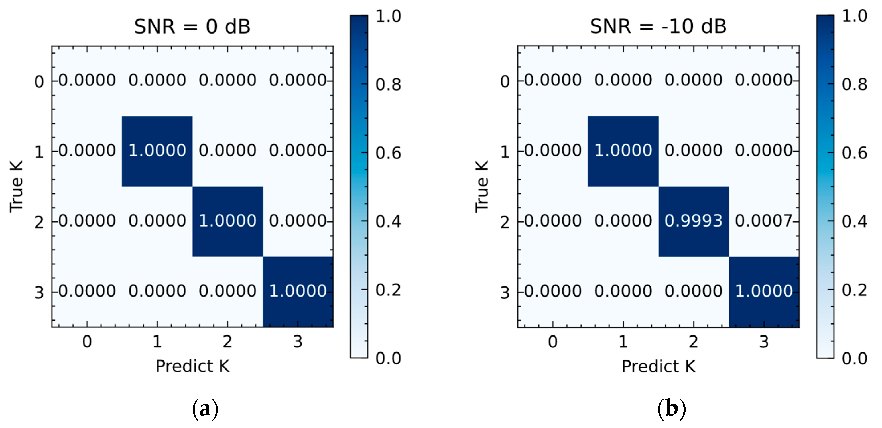
The tests were performed using fixed off-grid angles ranging from source number K = 1 to K = 3. For each K   , 10,000 test samples were independently generated with 1000 snapshots to form test sets at 0 dB, −10 dB, and −15 dB, respectively. The angles of first signal, second, and third were 3.74 , 11.11 , and 2.12 , respectively. The predicted K and their DOAs are obtained by filtering with a threshold p 0 and identifying peaks on probability spectrum output H ^ ( i ) in Equation (6). The results are reported in Table 1, which evaluates the performance of CNN-SCL with mean and max Hausdorff distance. When the SNR is 0 dB, the model firmly predicts { 4 , 11 , 2 }, resulting in the mean and max Hausdorff distance being fixed on 0.26 . At −10 dB, the errors are slightly increased but still small, considering the low SNR, while the state-of-the-art CNN approaches obtains high max d H of 10.8 in similar situation [12]. In the −15 dB SNR scenario, the maximum value of the Hausdorff distance increases significantly, and it varies with the number of sources. To avoid falsely identifying a zero target, the threshold value for the one-source scenario is set to 0.2 instead of 0.4, as the latter would result in a 0.53% probability of predicting zero targets. Additionally, Figure 3 indicates the confusion matrix (probability) of source predicted results with respect to 0 dB and −10 dB SNR. When predicting source number in low SNR environments, the model achieves this with only a 0.07% error rate in two-sources scenarios { 3.74 , 11.11 } in −10 dB SNR, indicating that our approach achieves high accuracy low SNR environments. In contrast to our CNN-SCL approach, the AIC method has proven to be ineffective in low SNRs [23]. Moreover, the only-CNN-based method retains an error rate of 22.47% for three-source scenario with a similar separation of angles at −10 dB SNR [12]. Compared to the current learning-based spectrum reconstruction method outlined in [13], our approach demonstrates superior accuracy, reducing the error rate significantly. However, our method does have its limitations. First, it is heavily data-driven, which substantially increases the volume of data required. This means hugely increasing the amount of required data. For instance, to predict four targets, we need to add extra 121 4 samples to the dataset, and 121 5 for five targets. Furthermore, as the array’s element count grows, the matrix size of every data point grows at a quadratic rate. In contrast, learning-based spectrum methods can more seamlessly adapt to various target counts and array sizes.

4.2. Known Number of Sources

In the given sources number setting, the experiments were conducted on two-source scenarios with varying SNRs and snapshots. In this case, the output selection approach is modified to choose the two highest values in the probability spectrum without prior filtering. The loss metric used is the RMSE. The performance of the proposed approach is evaluated against existing classical and state-of-the-art methods, and the Cramér–Rao lower bound (CRLB) [24] is provided as benchmark. Additionally, to examine the influence of SCL in proposed approach, the framework without SCL pretraining was evaluated and denoted as CNN-SCL w/o. All the on-grid approaches were set with resolution for one degree of every integer on [ 60 , 60 ] .

4.2.1. RMSE under Varying SNRs

The objective of this experiment is to estimate the DOAs of two sources at different SNRs while keeping the snapshots fixed at 1000. Each data point was tested with 1000 samples. The directions are 10.11 and 12.7 , respectively. The results are shown on Figure 4a. The proposed model exhibits relatively good performance when compared with the CNN in low-SNR regime, with RMSE values of 1.9910 , 0.6253 , and 0.5885 for −20 dB, −15 dB, and −10 dB, respectively. In the high-SNR regime, on-grid methods suffer from grid mismatch and exhibit high RMSE values, while grid-less methods, such as ESPRIT and R-MUSIC, approach the CRLB.

4.2.2. RMSE versus Varying Snapshots

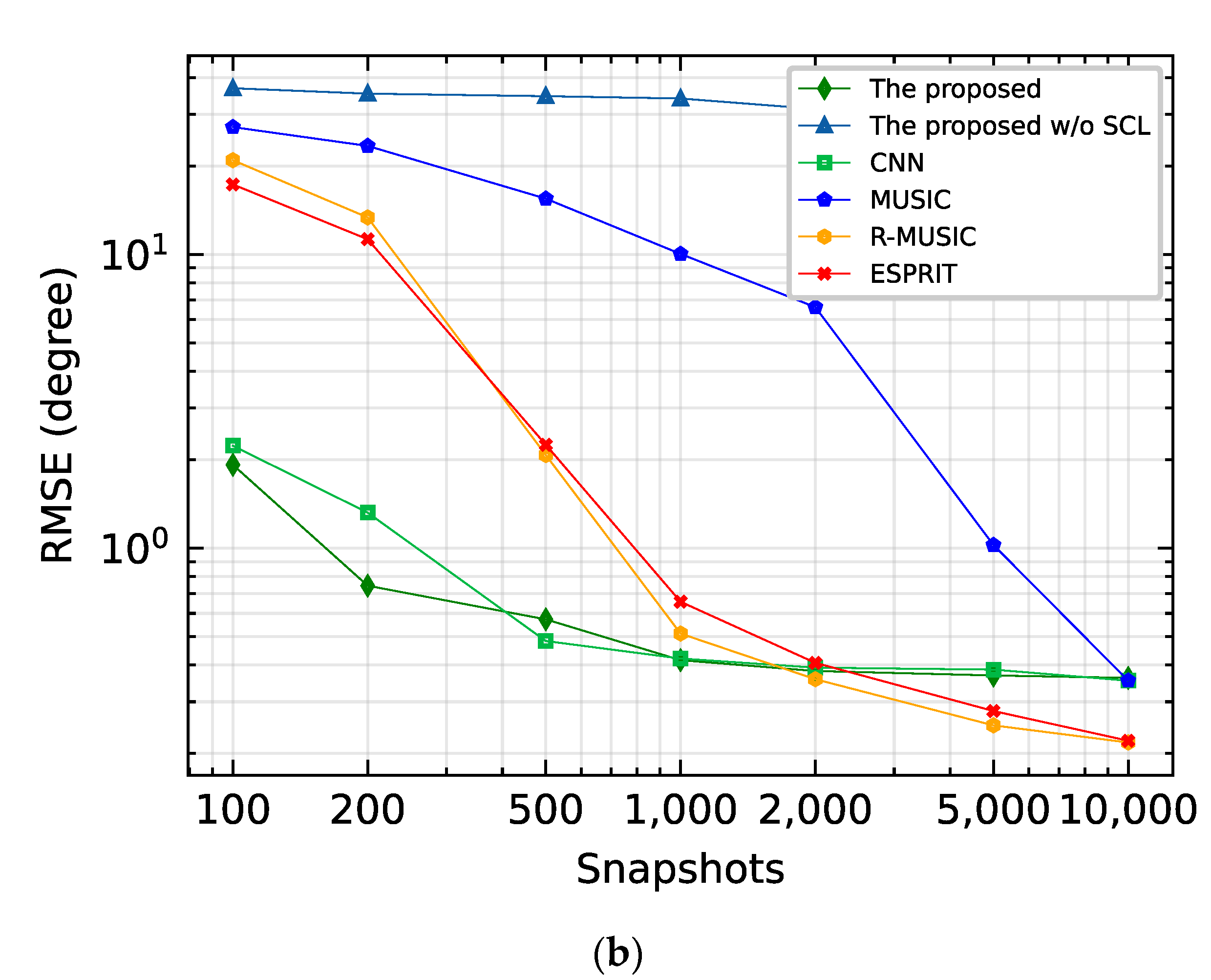
In this experiment, tests were conducted with two sources at −10 dB SNR while the snapshots ranged from 100 to 10,000. Each datapoint was tested with 1000 samples, with the directions being 9.58 and 12.82 , respectively. Figure 4b illustrates the results. The proposed model achieved superior accuracy at 100 and 200 snapshots, with error of 1.922 and 0.7451 , respectively.

5. Analysis

5.1. Latent Space Visualization

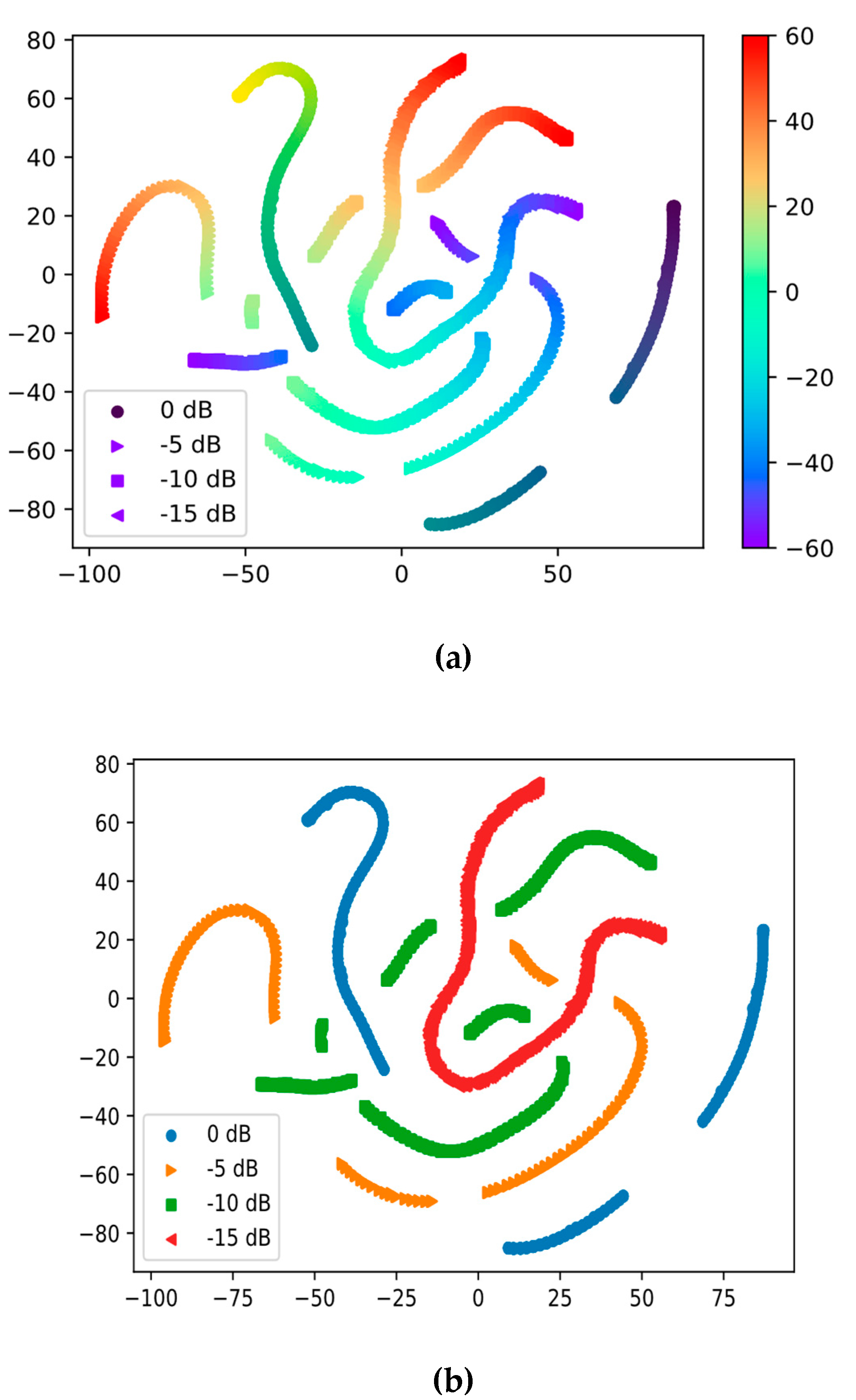
In both experiments conducted with varying SNRs and Snapshots, the framework CNN-SCL w/o without SCL pretraining was found to be difficult to converge. The pretraining was identified as the key factor causing this difference. To investigate the impact of pretraining, t-SNE [25] was employed to visualize the features distribution in latent space Z = f ( X ) during both the pretraining stage and training stage by mapping distribution into low-dimensional space while retaining relative distance between data points as much as possible. The values and colors represent the distributions and DOAs of input matrices X. Figure 5a depicts the messy distribution of data processed by the feature extractor without pretraining, whereas the distribution of different classes of angles is well separated by the SCL-pretrained feature extractor, as Figure 5b illustrates. Furthermore, after the training stage with classifier, SCL-pretrained feature extractor separates the features more clearly, forming gradual and continuous distribution, as shown in Figure 5c. As the model only utilizes nearly one-sixteenth of parameters compared with CNN [12], the direct training is hard to fit the data. However, the SCL pretraining provides the feature extractor with a good starting point, as shown in Figure 5b, which enables the training step to proceed more smoothly. This results in the stripe pattern being stretched, as shown in Figure 5c, thus leading to a clear and robust decision boundary. The SCL pretraining enhances parameter efficiency, performance, and generalization in low-SNR DOA estimation. In Figure 6, we visualize the distribution of DOA data after processing through the CNN extractor under various SNR conditions. The findings indicate that the SCL-CNN extracts DOA information based on an amplitude-phase pattern. As illustrated in Figure 6a, when the angle approaches 0, implying minimal phase difference between the array elements, the distribution tends to be closer to the inner side of the center. In Figure 6b, we differentiated data points based on varying SNR levels. It was observed that features extracted from DOA data with lower SNR tend to be located closer to the center. This observation implicitly corroborates the assertions made in the paper [26], suggesting that the information extraction from CNN follows the pattern of pseudospectrum construction in the MUSIC method, where features are extracted based on amplitude and phase and then arranged in ascending order.

5.2. Feature Learning for Analysis

From the theoretical perspective, the recent advancement [27,28,29] of neural network approximation also provides some intuition for explaining the shift of distribution in Figure 5. In paper [27], Allen-Zhu and Li (2020) demonstrated a novel theoretical framework that characterized the feature learning process of neural networks, which is adopted in paper [28], where Cao et al. (2022) leveraged that framework to analyze the behavior of neural networks under various SNR. Furthermore, in paper [29], Chen Y et al. (2023) go further in analyzing the learning processing of model between spurious and invariant features. The convolutional neural network model analyzed by papers [28,29] is only comprised of two layers at any width, and the deeper neural networks still need further study and investigation. However, as the deeper networks are always more powerful than shallow neural networks in practice, and because they need fewer parameters or units to achieve the same effect as shallow networks [30], we assume that our network can easily fulfill the equivalent conditions that paper [28,29] requests. Thus, the lemmas shall be reasonable to be applied in explaining the effect of pretrain in Figure 5 intuitively.
We consider the simplified model and data set for analysis, which is adopted from papers [28,29]. The analysis focuses on how to suppress the spurious feature and learn the invariant feature in order to achieve Out-of-Distribution (OOD) generalization, namely generalization to other distributions other than the training data set. The spurious features are always correlated with the invariant feature but with contribute negligible information for prediction or estimation. In contrast to the spurious feature, the invariant feature points out the characteristics that are informative and stable inside data. Considering the form of DOA estimation data and matrices are similar to a picture with multiple channels, it is plausible to assume the existence of spurious features.

5.2.1. Preliminary and Ideal Model

Suppose the data set for the ideal model is D = x i , y i i = 1 n , where n is the number of samples, d is the dimension x   R 2 d , and y   { 1,1 } . The input data instances ( x i , y i ) conform to the following distribution:
  • The label y   is generated as a Rademacher random variable.
  • Given y   , each input x   = { x 1 , x 2 } include a feature patch x 1 and a noise patch x 2 , that are sampled as:
    x 1 = y Ra d α v 1 + y Ra d β v 2 x 2 = ξ
    where Ra d x presenting the random variable taking value 1 with probability 1-x and −1 with probability x. v 1 = [ 1,0 , 0 , 0 ] and α is usually constant, representing the invariant feature; v 2 = [ 0,1 , 0 , 0 ] and β is usually uncertain with different data, representing the spurious feature with unreliable information.
  • The noise vector conforms to the Gaussian distribution N 0 , σ p 2 I d v 1 v 1 v 2 v 2 , indicating a noise orthogonal with both spurious and invariant features.
An ideal two-layer CNN model is trained to classify the label with sigmoid and cross-entropy loss function, the network can be written as f ( W , x ) = F + 1 W + 1 , x F 1 W 1 , x , with:
F j W j , x = 1 m r = 1 m σ w j , r x 1 + σ w j , r x 2
where σ ( x ) is the activation function.

5.2.2. Theorem and Intuition

Lemma 1
(Cao et al. [28]; Chen et al. [29]). Let w j , r ( t ) for j { + 1 , 1 } and r { 1,2 , 3 , . . . m } be the convolution filters of the CNN at t-th iteration of gradient descent. Then there exists unique coefficients γ j , r , 1 ( t ) , γ j , r , 2 ( t ) 0 and ρ j , r , i ( t ) s.t.:
w j , r t = w j , r 0 + j γ j , r , 1 t v 1 + j γ j , r , 2 t v 2 + ρ j , r , i t ξ i 2 2 ξ i
Lemma 1 is the basis for following lemmas. It reveals the behavior of neural networks when updated. The weights are the time-varying linear combination of initialized weights w j , r 0 , invariant signal v 1 , spurious signal v 2 , and noise ξ i . As w j , r 0 0 and the rest of the components are orthogonal to each other, γ j , r , 1 w j , r , v 1 and γ j , r , 2 w j , r , v 2 learning progress of invariant feature and spurious feature.
Lemma 2
(Chen et al. [29]). For two samples   x 1 e , x 1 e . With invariant risk minimization regularization c ( t ) , define λ 0 = λ m i n H ,   where   H e , e 1 2 m n e n e i = 1 n e x 1 , i e i = 1 n e x 1 , i e . Suppose that dimension d = Ω ( l o g ( m / δ ) ) , network width m = Ω ( 1 / δ ) , regularization factor λ 1 / σ 0 , noise variance σ p = O d 2 , weight initial scale σ 0 = O m i n λ 0 2 m 2 l o g ( 1 / ϵ ) , λ 0 m d l o g ( 1 / ϵ ) , then with probability at least 1 δ , after training iteration T = Ω l o g ( 1 / ϵ ) η λ λ 0 , we have:
c T 2 ϵ , γ j , r , 1 T = o d 1 , γ j , r , 2 T = o d 1
The theorem demonstrates that heavy invariant risk minimization (IRM) regularization hinders the learning process for both spurious and invariant features. The loss stays at constant at the same time. IRM aims to find the invariant feature under whatever possible feature distribution [31]. We observe that the strong weights-share regularization [18] of our CNN-SCL model in the first four FC layers play similar roles as IRM, which not only rise the generalization of the model but the difficulty of training, keeping the training and testing loss as relatively large constant in Figure 4 term CNN-SCL w/o.
Lemma 3
(Chen et al. [29]). Suppose spurious correlations are stronger than invariant correlations α > β , and γ j , r i n v t 1 = γ j , r i n v t 1 1 and γ j , r s p u t 1 = γ j , r s p u t 1 1 at the end of pretraining iteration t 1 . Suppose that δ > 0 and n > C l o g ( 1 / δ ) , with C being a positive constant, then with a high probability at least 1 δ , we have regularization loss approaches zero and γ j , r i n v t 1 + 1 > γ j , r i n v t 1 while γ j , r s p u t 1 + 1 < γ j , r s p u t 1 .
This lemma indicates that the learning processing can start learning process with the strong and enough pretraining, even under heavy regularization. And in the training stage after pretraining stage, the learned invariant feature would be empowered, while the spurious feature would be suppressed. Thus, we can observe the CNN-SCL with pretraining perform better than CNN-SCL w/o in Figure 4.
In Figure 5a–c, the manifestation of the pattern further validates the effect that Lemma 2 and Lemma 3 point out. In Figure 5a, as Lemma 2 reveals, CNN-SCL w/o incurs heavy regularization, performs worst feature distribution, and learns almost nothing. In Figure 5b, as Lemma 3 suggests, supervised contrastive learning is a very powerful pretraining method to help the model overcome regularization and start learning both spurious and invariant features, so the pattern begins to separate and order. Finally, as Lemma 3 indicates, Figure 5c illustrates that with enough training after pretraining, the invariant features have been learned and the spurious features were suppressed, from which a clear and robust feature distribution forms.

6. Conclusions

In this paper, we introduced a new framework called CNN-SCL for on-grid multi-target DOA estimation in low SNRs and limited snapshots. The proposed method is based on contrastive learning, which aims to separate different features with a regular pattern. The experimental results demonstrate the robustness and generalization capability of our proposed method, outperforming other methods in harsh environments for both number of source classifications and DOA estimations. The analysis confirms the necessity of SCL pretraining in both visualization and theory. Additionally, our approach achieves comparable performance with state-of-the-art methods while number of parameters significantly decreases near 94%. Our future work will focus on exploring the potential of contrastive learning to further reduce the parameters for DOA estimation with deep learning.

Author Contributions

Conceptualization, C.C. and Y.L.; methodology, Z.Z. (Zhengjie Zhou); software, Z.Z. (Zhiquan Zhou) and P.W.; validation, Y.L., C.C. and Z.Z. (Zhiquan Zhou); formal analysis, Z.Z. (Zhengjie Zhou); investigation, Z.Z. (Zhengjie Zhou); resources, Z.Z. (Zhengjie Zhou); data curation, Z.Z. (Zhengjie Zhou); writing—original draft preparation, Z.Z. (Zhengjie Zhou); writing—review and editing, Y.L. and C.C.; visualization, Z.Z. (Zhengjie Zhou); supervision, Y.L.; project administration, Y.L.; funding acquisition, Y.L. All authors have read and agreed to the published version of the manuscript.

Funding

This research was funded by the National Natural Science Foundation of China, grant number [62001143]; the National Natural Science Foundation of Shandong Province, grant number [ZR2020QF006, ZR201910220437]; the Major Scientific and technological innovation project of Shandong Province, grant number [2021ZLGX05, 2022ZLGX04].

Data Availability Statement

Data that support the finding of this study are available from the first author upon reasonable request ([email protected]).

Conflicts of Interest

The authors declare that they have no known competing financial interests or personal relationships that could have appeared to influence the work reported in this paper.

References

  1. Schmidt, R. Multiple emitter location and signal parameter estimation. IEEE Trans. Antennas Propag. 1986, 34, 276–280. [Google Scholar] [CrossRef]
  2. Roy, R.; Kailath, T. ESPRIT-estimation of signal parameters via rotational invariance techniques. IEEE Trans. Acoust. Speech Signal Process. 1989, 37, 984–995. [Google Scholar] [CrossRef]
  3. Rao, B.D.; Hari, K.V.S. Performance analysis of root-MUSIC. IEEE Trans. Acoust. Speech Signal Process. 1989, 37, 1939–1949. [Google Scholar] [CrossRef]
  4. Liu, T. Porosity reconstruction based on Biot elastic model of porous media by homotopy perturbation method. Chaos Solitons Fractals 2022, 158, 112007. [Google Scholar] [CrossRef]
  5. Liu, T.; Ding, Z.; Yu, J.; Zhang, W. Parameter Estimation for Nonlinear Diffusion Problems by the Constrained Homotopy Method. Mathematics 2023, 11, 2642. [Google Scholar] [CrossRef]
  6. Liu, T.; Yu, J.; Zheng, Y.; Liu, C.; Yang, Y.; Qi, Y. A nonlinear multigrid method for the parameter identification problem of partial differential equations with constraints. Mathematics 2022, 10, 2938. [Google Scholar] [CrossRef]
  7. Liu, T.; Ouyang, D.; Guo, L.; Qiu, R.; Qi, Y.; Xie, W.; Ma, Q.; Liu, C. Combination of Multigrid with Constraint Data for Inverse Problem of Nonlinear Diffusion Equation. Mathematics 2023, 11, 2887. [Google Scholar] [CrossRef]
  8. Liu, T. Parameter estimation with the multigrid-homotopy method for a nonlinear diffusion equation. J. Comput. Appl. Math. 2022, 413, 114393. [Google Scholar] [CrossRef]
  9. Kumchaiseemak, N.; Chatnuntawech, I.; Teerapittayanon, S.; Kotchapansompote, P.; Kaewlee, T.; Piriyajitakonkij, M.; Wilaiprasitporn, T.; Suwajanakorn, S. Toward Ant-Sized Moving Object Localization Using Deep Learning in FMCW Radar: A Pilot Study. IEEE Trans. Geosci. Remote Sens. 2022, 60, 1–10. [Google Scholar] [CrossRef]
  10. Kase, Y.; Nishimura, T.; Ohgane, T.; Ogawa, Y.; Kitayama, D.; Kishiyama, Y. DoA estimation of two targets with deep learning. In Proceedings of the 2018 15th Workshop on Positioning, Navigation and Communications (WPNC), Bremen, Germany, 25–26 October 2018; pp. 1–5. [Google Scholar]
  11. Liu, Z.M.; Zhang, C.; Philip, S.Y. Direction-of-arrival estimation based on deep neural networks with robustness to array imperfections. IEEE Trans. Antennas Propag. 2018, 66, 7315–7327. [Google Scholar] [CrossRef]
  12. Papageorgiou, G.K.; Sellathurai, M.; Eldar, Y.C. Deep networks for direction-of-arrival estimation in low SNR. IEEE Trans. Signal Process. 2021, 69, 3714–3729. [Google Scholar] [CrossRef]
  13. Lee, K. Deep learning-aided coherent direction-of-arrival estimation with the FTMR algorithm. IEEE Trans. Signal Process. 2022, 70, 1118–1130. [Google Scholar]
  14. Wu, X.; Yang, X.; Jia, X.; Tian, F. A gridless DOA estimation method based on convolutional neural network with Toeplitz prior. IEEE Signal Process. Lett. 2022, 29, 1247–1251. [Google Scholar] [CrossRef]
  15. Oord, A.; Li, Y.; Vinyals, O. Representation learning with contrastive predictive coding. arXiv 2018, arXiv:1807.03748. [Google Scholar]
  16. Khosla, P.; Teterwak, P.; Wang, C.; Sarna, A.; Tian, Y.; Isola, P.; Maschinot, A.; Liu, C.; Krishnan, D. Supervised contrastive learning. Adv. Neural Inf. Process. Syst. 2020, 33, 18661–18673. [Google Scholar]
  17. Gu, J.; Wang, Z.; Kuen, J.; Ma, L.; Shahroudy, A.; Shuai, B.; Liu, T.; Wang, X.; Wang, G.; Cai, J.; et al. Recent advances in convolutional neural networks. Pattern Recognit. 2018, 77, 354–377. [Google Scholar] [CrossRef]
  18. Nowlan, S.J.; Hinton, G.E. Simplifying neural networks by soft weight-sharing. Neural Comput. 1992, 4, 473–493. [Google Scholar] [CrossRef]
  19. Cubuk, E.D.; Zoph, B.; Mane, D.; Vasudevan, V.; Le, Q.V. Autoaugment: Learning augmentation policies from data. arXiv 2018, arXiv:1805.09501. [Google Scholar]
  20. Hassani, K.; Khasahmadi, A.H. Contrastive multi-view representation learning on graphs. In Proceedings of the International Conference on Machine Learning, Virtual Event, 13–18 July 2020; pp. 4116–4126. [Google Scholar]
  21. Kingma, D.P.; Ba, J. Adam: A method for stochastic optimization. arXiv 2014, arXiv:1412.6980. [Google Scholar]
  22. Nitzberg, R. Constant-false-alarm-rate signal processors for several types of interference. IEEE Trans. Aerosp. Electron. Syst. 1972, 27–34. [Google Scholar] [CrossRef]
  23. Wong, K.M.; Zhang, Q.T.; Reilly, J.P.; Yip, P.C. On information theoretic criteria for determining the number of signals in high resolution array processing. IEEE Trans. Acoust. Speech Signal Process. 1990, 38, 1959–1971. [Google Scholar] [CrossRef]
  24. Stoica, P.; Nehorai, A. Performance study of conditional and unconditional direction-of-arrival estimation. IEEE Trans. Acoust. Speech Signal Process. 1990, 38, 1783–1795. [Google Scholar] [CrossRef]
  25. Van der Maaten, L.; Hinton, G. Visualizing data using t-SNE. J. Mach. Learn. Res. 2008, 9. [Google Scholar]
  26. Adavanne, S.; Politis, A.; Virtanen, T. Direction of arrival estimation for multiple sound sources using convolutional recurrent neural network. In Proceedings of the 2018 26th European Signal Processing Conference (EUSIPCO), Rome, Italy, 3–7 September 2018; IEEE: Piscataway, NJ, USA, 2018; pp. 1462–1466. [Google Scholar]
  27. Allen-Zhu, Z.; Li, Y. Towards understanding ensemble, knowledge distillation and self-distillation in deep learning. arXiv 2020, arXiv:2012.09816. [Google Scholar]
  28. Cao, Y.; Chen, Z.; Belkin, M.; Gu, Q. Benign overfitting in two-layer convolutional neural networks. Adv. Neural Inf. Process. Syst. 2022, 35, 25237–25250. [Google Scholar]
  29. Chen, Y.; Huang, W.; Zhou, K.; Bian, Y.; Han, B.; Cheng, J. Towards Understanding Feature Learning in Out-of-Distribution Generalization. arXiv 2023, arXiv:2304.11327. [Google Scholar]
  30. Liang, S.; Srikant, R. Why deep neural networks for function approximation? arXiv 2016, arXiv:1610.04161. [Google Scholar]
  31. Arjovsky, M.; Bottou, L.; Gulrajani, I.; Lopez-Paz, D. Invariant risk minimization. arXiv 2019, arXiv:1907.02893. [Google Scholar]
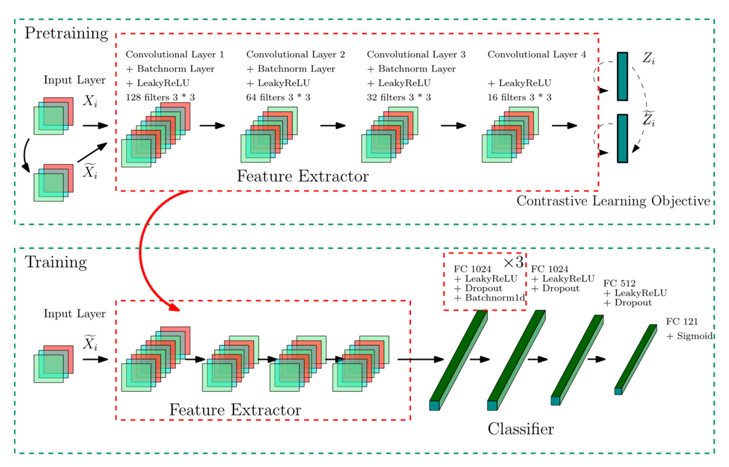
Figure 1. The SCL-based architecture, including pretraining and training. Dropout probability is set to 0.2 and the stride of all convolution filters is 1. The LeakyReLU applies 0.01 negative slope. The first four fully connected layers of Classifier share the same weights. After the pretraining stage, the pretrained feature extractor will be trained with an initialized classifier. The numbers of neurons of fully connected layers are labeled above.
Axioms 12 00862 g001
Figure 2. (a) Pretraining loss curve; (b) Training loss curve.
Axioms 12 00862 g002
Figure 3. (a) Confusion matrix in 0 dB; (b) Confusion matrix in −10 dB.
Axioms 12 00862 g003
Figure 4. (a) Two-target RMSE loss versus SNRs; (b) Two-target RMSE loss versus Snapshots.
Axioms 12 00862 g004aAxioms 12 00862 g004b
Figure 5. Distributions of output feature from feature extractors with respect to angles at −10 dB, 100 snapshots. (a) without SCL pretraining, directly trained with classifier; (b) with SCL pretraining only; (c) with SCL-pretrained and then further trained with classifier.
Axioms 12 00862 g005
Figure 6. Distributions of output feature from feature extractors with respect to angles at 0 dB, −5 dB, −10 dB and −15 dB, 1000 snapshots. (a) with SCL-pretrained and then further trained with classifier, DOA distribution; (b) with SCL-pretrained and then further trained with classifier, SNR distribution.
Axioms 12 00862 g006
Table 1. Unknown target estimation in 0 dB, −10 dB, and −15 dB.
Number of Sources K 1 Threshold   p 0 Mean   d H (Degree) Max   d H (Degree)
SNR = 0 dB
10.40.2600 0.2600
20.40.2600 0.2600
30.40.2600 0.2600
SNR = −10 dB
10.40.26590.7400
20.40.27891.2600
30.40.3052 1.1200
SNR = −15 dB
10.20.406223.74
20.40.473715.11
30.40.746310.11
1 We further tested the false alarm rate of zero target on standard white noise with the same snapshots, 10,000 samples, and Threshold p 0 = 0.4. Under zero-target conditions, there is only a 0.09% chance of mistakenly counting it as one target signal source while 99.91% counting correct.
Disclaimer/Publisher’s Note: The statements, opinions and data contained in all publications are solely those of the individual author(s) and contributor(s) and not of MDPI and/or the editor(s). MDPI and/or the editor(s) disclaim responsibility for any injury to people or property resulting from any ideas, methods, instructions or products referred to in the content.