Article

Reliability Estimation of Inverse Weibull Distribution Based on Intuitionistic Fuzzy Lifetime Data

1
College of Science, Jiangxi University of Science and Technology, Ganzhou 341000, China
2
Teaching Department of Basic Subjects, Jiangxi University of Science and Technology, Nanchang 330013, China
*
Author to whom correspondence should be addressed.
Axioms 2023, 12(9), 838; https://doi.org/10.3390/axioms12090838
Submission received: 27 June 2023 / Revised: 17 August 2023 / Accepted: 26 August 2023 / Published: 29 August 2023
(This article belongs to the Special Issue Mathematical Methods in the Applied Sciences)

Abstract

:
As a commonly used model in reliability analysis, the inverse Weibull distribution (IWD) is widely applied in various scientific fields. This paper considers the reliability estimation of the IWD based on intuitionistic fuzzy lifetime data. Firstly, the related concepts of the fuzzy set theory are reviewed, and the concepts of the intuitionistic fuzzy conditional density, intuitionistic fuzzy likelihood function, and intuitionistic fuzzy conditional expectation are obtained by extension. In classical estimations, the maximum likelihood estimators of parameters and reliability are derived. Due to the nonlinearity, the EM algorithm is used to obtain the maximum likelihood estimates. In the Bayesian estimation, the gamma prior is selected, and the Bayesian estimation of the parameters and reliability is conducted under the symmetric entropy and the scale square error loss function, respectively. Since the integrals are complicated, the Lindley approximation is used to approximate the Bayesian estimates. Then, the performance of these estimators is evaluated by the Monte Carlo simulation. The simulation results show that the Bayesian estimation is more suitable than the maximum likelihood estimation for the reliability estimation. Finally, a set of real data is used to prove the effectiveness of these proposed methods. Through these methods, the reliability of the intuitive fuzzy life data is accurately estimated, which provides an important reference for the reliability analysis in the scientific field.

1. Introduction

Reliability refers to the ability of a product to complete the specified tasks under the specified time and conditions. This is a theory based on product failure. Due to the existence of two parameters, the IWD is a very flexible life distribution that can be used to represent various failure characteristics. It has become one of the commonly used models in reliability analysis. Depending on the shape parameter, the risk function can be flexibly varied. Therefore, it is appropriate to use IWD for data fitting in many cases. Yilmaz and Kara [1] investigated the classical and Bayesian estimation methods for estimating the reliability of IWD. The classical approach involved obtaining the maximum likelihood estimation and the modified maximum likelihood estimation. Meanwhile, the Bayesian estimation method under symmetric and asymmetric loss functions was considered. The Bayes estimators were computed numerically using the Lindley approximation and MCMC algorithm. Chakrabarty and Chowdhury [2] analyzed two probability distributions formed by compounding the IWD with zero-truncated Poisson and geometric distributions, respectively. They derived some important statistical and reliability attributes for each distribution and estimated the parameters of the distributions using the expectation–maximization algorithm and minimum distance estimation method. Cai et al. [3] investigated the statistical inference of the IWD with masked data in a series system under type-II censoring. They obtained Bayes estimators of parameters based on gamma priors, as well as multilevel Bayes estimators. Finally, they conducted a Monte Carlo simulation with different masking probabilities and effective sample sizes to compare the performances of various estimates. Bi and Gui [4] considered the stress-strength reliability estimation of an inverse Weibull lifetime model with identical shape parameters but different scale parameters. In terms of the classical estimation, maximum likelihood estimators and asymptotic distributions were obtained. As the estimators were in implicit forms, an approximate maximum likelihood estimator was proposed, and asymptotic confidence intervals were obtained. In terms of the Bayesian estimation, Bayes estimators were obtained by Gibbs sampling and the MH algorithm. The performance of each estimator was compared through Monte Carlo simulations. For an additional reliability analysis of the IWD, please refer to [5,6,7,8,9].
The key to reliability estimation lies in collecting lifetime data or transforming other reliability data collected into lifetime data. However, in the process of obtaining the data, there may be some degree of measurement errors, resulting in imprecise data collection. In 1965, Zadeh [10] introduced the fuzzy set theory, which offered a proper tool for handling inaccurate data. The importance of fuzzy sets lies in their ability to handle uncertainties and vagueness, making them valuable mathematical tools in fields, such as artificial intelligence, control theory, and decision analysis [11,12,13,14,15,16,17]. By using fuzzy sets, we can translate vague information from the real world into mathematical language, allowing for precise calculations and reasoning. In recent years, some scholars have extended the fuzzy set theory to reliability analysis. Hashim [18] considered the problem of the fuzzy reliability estimation for the Lomax distribution. The first step was to use the composite trapezoidal rule to estimate the fuzzy reliability based on its definition. The second step was the Bayesian estimation method, where a gamma prior was selected to estimate the fuzzy reliability under symmetric and asymmetric loss functions. Neamah and Ali [19] considered the parameter estimation for the Frechet distribution of fuzzy lifetime data. Maximum likelihood and Bayes estimators were obtained for both parameters and reliability. Through a comparison of the mean squared error and mean absolute percentage error, it was found that the performance of the Bayesian estimation was better than that of the maximum likelihood estimation. Abbas et al. [20] studied the Bayesian estimation of the parameters of the Rayleigh distribution for fuzzy lifetime data. As an explicit form of the Bayes estimator could not be obtained, Lindley and Tierney–Kadane approximations were used for the numerical computation. Monte Carlo simulations were conducted to evaluate their performance, and a set of examples were provided to illustrate the analysis.
However, fuzzy sets only use one attribute parameter (membership degree) to represent both support and opposition, and cannot represent a neutral state, i.e., neither supporting nor opposing. To address this, Atanassov [21] introduced the notion of the intuitionistic fuzzy set, which was an extension of Zadeh’s fuzzy set. Compared with traditional fuzzy sets, intuitionistic fuzzy sets add a new non-membership parameter, which can more delicately characterize the ambiguity inherent in the objectively defined world. When dealing with decision-making problems, intuitionistic fuzzy sets can provide more information, making the decision results more accurate and reliable, and have a wider range of application prospects [22,23,24,25,26]. Zahra et al. [27] considered the parameter and reliability estimation of the Pareto distribution by setting the parameter as a generalized intuitionistic fuzzy number. First, an L-R-type intuitionistic fuzzy number was proposed, and its cut set was provided. Secondly, a series of generalized intuitionistic fuzzy reliability characteristics were defined and used to evaluate the reliability of series and parallel systems. Finally, generalized intuitionistic fuzzy reliability characteristics were provided for certain special parameters and cut-set cases. Ebrahimnejad and Jamkhaneh [28] considered the reliability estimation problem of the Rayleigh distribution by assuming the parameter as a generalized intuitionistic fuzzy number. Extending the fuzzy reliability concept, a series of generalized intuitionistic fuzzy reliability characteristics and their cut sets were provided, and a numerical example was provided to demonstrate the analysis.
There are many uncertainties in real-life phenomena, which are usually classified into three categories: randomness, fuzziness, and roughness. However, in many cases, multiple types of uncertainties are at play, making it impossible to solve these problems using only one uncertainty theory. Fuzzy stochastic phenomena, which are common in real life, are the result of the simultaneous interaction of randomness and fuzziness, and their study is of great significance. To better handle this phenomenon, the fuzzy stochastic theory has emerged, which is a theory combining the fuzzy set and probability theories. One of its important concepts is the fuzzy random variable proposed by Huibert [29]. Zahra et al. [30] extended the definitions of probability, conditional probability, and likelihood function to intuitionistic fuzzy observations, and considered the parameter and reliability function estimation problem of the two-parameter Weibull distribution based on intuitionistic fuzzy lifetime data. ML estimators were obtained using the Newton–Raphson and EM algorithms, and Bayes estimators were obtained using Lindley and Tierney–Kadane approximations. To demonstrate the applicability of the proposed estimation methods, a simulation dataset was analyzed.
In terms of the reliability estimation for the IWD, many scholars have conducted research; however, most of them are based on complete or censored samples, and these studies assume that the available data are precise. However, in real life, the available lifetime data may not be precise, which indicates the necessity of extending classical estimation methods to fuzzy numbers.
The main contribution of this paper is to provide a suitable estimation method for the parameters and reliability of IWD based on intuitionistic fuzzy lifetime data. For the classical estimation, we obtain MLEs for the parameters and reliability. Due to the nonlinearity of the likelihood equation, we provide the EM algorithm with specific iteration steps. For the Bayesian estimation, we obtain BEs of parameters and reliability under the SE loss and SSE loss functions. The approximate Bayesian estimates are obtained by the Lindley approximation. Based on several sets of different parameter values and a large number of simulation experiments, the simulation results show that the Bayesian estimation performs much better than the maximum likelihood estimation.
This paper considers the reliability estimation problem of the IWD based on intuitionistic fuzzy lifetime data. In Section 1, the article mainly introduces the research status of the reliability estimation of the IWD lifetime model, as well as the research background and significance of fuzzy sets and intuitionistic fuzzy sets. Section 2 reviews the concepts of fuzzy sets and intuitionistic fuzzy sets, and extends some important concepts of the probability theory to the fuzzy set theory. Section 3 performs the maximum likelihood estimators (MLEs) of IWD, and iteratively calculates them using the expectation–maximization (EM) algorithm. Section 4 performs the Bayes estimators (BEs) under the symmetric entropy (SE) loss function and scale squared error (SSE) loss function, and numerically calculates the results using the Lindley approximation. Section 5 evaluates the performance of each estimation method using the Monte Carlo simulation and illustrates it using the mean squared error (MSE). The feasibility of the proposed methods is verified by a real dataset in Section 6. Section 7 presents the conclusions, limitations, and future research.

2. Preliminary Knowledge

The probability density function (pdf), cumulative distribution function (cdf), and reliability function of IWD are defined, respectively, as:
y ( t ; λ , η ) = λ η t η 1 exp ( λ t η ) ,   t > 0 ,
Y ( t ; λ , η ) = exp ( λ t η ) ,   t > 0 ,
R ( t ) = 1 exp ( λ t η ) ,   t > 0 ,
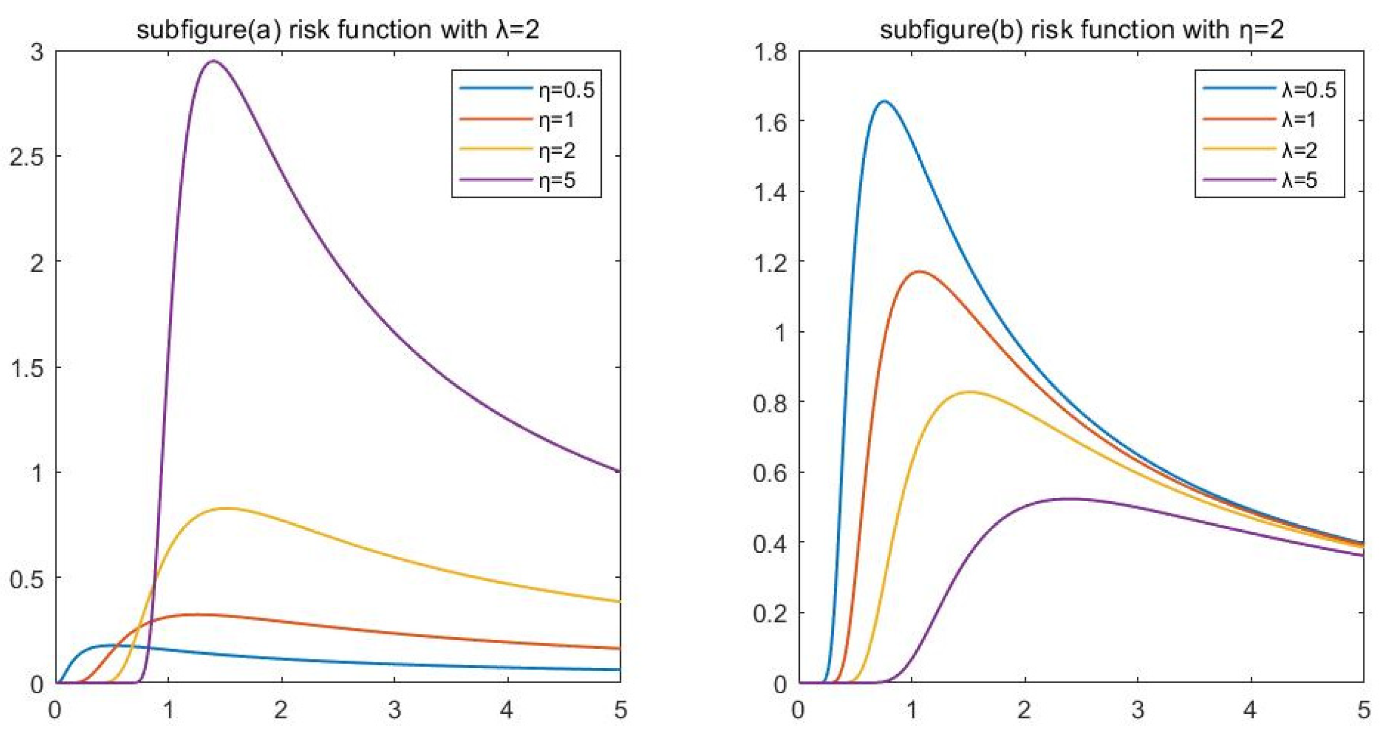
where λ > 0 is the scale parameter and η > 0 is the shape parameter. For convenience, denote IWD owing pdf (1) by IW ( λ , η ) . Figure 1 and Figure 2 show the pdf and risk function under different values of the shape and scale parameters.
A fuzzy set is a set used to express the concept of fuzziness. Similar to the definition of the characteristic function of the classical set, the definition of fuzzy set can be obtained by extending its domain.
Definition 1 
(Zadeh [10]). Let T be a non-empty universal set. Fuzzy set A ˜ is defined as the form A ˜ = { < t , μ A ˜ ( t ) > | t T } , where μ A ˜ : T [ 0 , 1 ] is the degree of membership of t in A ˜ .
The intuitionistic fuzzy set (IFS) first proposed by Atanassov in 1986 contains two parameters, membership and non-membership degrees, which can more comprehensively describe the characteristics of things.
Definition 2 
(Atanassov [21]). Let T be a non-empty universal set. IFS A ˜ is defined as the form A ˜ = { < t , μ A ˜ ( t ) , ν A ˜ ( t ) > | t T } , where μ A ˜ : T [ 0 , 1 ] is the degree of membership of t in A ˜ and ν A ˜ : T [ 0 , 1 ] is the degree of non-membership of t in A ˜ . They satisfy 0 μ A ˜ ( t ) + ν A ˜ ( t ) 1 for each t . When  T has only one element,  A ˜ = < μ A ˜ , ν A ˜ > is commonly referred to as a intuitionistic fuzzy number.
Two special classes of intuitionistic fuzzy numbers are triangular intuitionistic fuzzy numbers (TriIFNs) and trapezoidal intuitionistic fuzzy numbers (TraIFNs), which serve as extensions of intuitionistic fuzzy numbers. In 2006, Shu et al. [31] proposed the definition of TriIFN and its application to fault tree analysis. Building on this work, Wang and Zhang [32] defined TraIFN in 2008. The membership and non-membership functions are:
μ A ˜ ( t ) = { α t a b a t [ a , b ] α t ( b , c ) α d t d c t [ c , d ] 0   else ,
ν A ˜ ( t ) = { b t b a + β t a b a t [ a , b ] β t ( b , c ) t c d c + β d t d c t [ c , d ] 1   else ,
where α is the maximum membership degree and β is the minimum membership degree.
In this paper, we assume T be a set of real numbers, which is T = . Additionally, we assumed that the IFSs discussed in this paper were TraIFNs.
To better investigate the estimation problem on the basis of intuitionistic fuzzy data, some concepts in the probability theory were extended to intuitionistic fuzzy random variables.
Definition 3. 
Consider a probability space  ( n , A , P ) , the probability of an intuitionistic fuzzy observation  x ˜  in  n  is defined by
P ( x ˜ ) = n 1 ν x ˜ ( t ) + μ x ˜ ( t ) 2 d P
Let the continuous random variable T = ( T 1 , T 2 , , T n ) obey the IW ( λ , η ) , and its intuitionistic fuzzy observations are denoted by x ˜ = ( x ˜ 1 , x ˜ 2 , , x ˜ n ) . The conditional density of random variables in probability theory is introduced, and the intuitionistic fuzzy conditional density is given as below,
y ( t | x ˜ ) = s ( t ) y ( t ; λ , η ) s ( t ) y ( t ; λ , η ) d t
where s ( t ) = 1 ν x ˜ ( t ) + μ x ˜ ( t ) 2 . In such a situation, the intuitionistic fuzzy likelihood function of IW ( λ , η ) is:
h ( λ , η | x ˜ ) = i = 1 n P ( x ˜ i | λ , η ) = i = 1 n s i ( t ) y ( t ; λ , η ) d t ,
where s i ( t ) = 1 ν x ˜ i ( t ) + μ x ˜ i ( t ) 2 .
Finally, intuitionistic fuzzy conditional expectation is introduced. Based on the intuitionistic fuzzy conditional density and intuitionistic fuzzy observation x ˜ = ( x ˜ 1 , x ˜ 2 , , x ˜ n ) , the intuitionistic fuzzy conditional expectation of a random variable T = ( T 1 , T 2 , , T n ) is:
E ( T | x ˜ ) = t y ( t | x ˜ ) d t = t s ( t ) y ( t ; λ , η ) s ( t ) y ( t ; λ , η ) d t d t = t s ( t ) y ( t ; λ , η ) h ( λ , η | x ˜ ) d t .

3. Maximum Likelihood Estimation

The intuitionistic fuzzy likelihood function of IW ( λ , η ) is shown in Equation (8). Thus, the intuitionistic fuzzy log-likelihood function is provided as:
H ( λ , η | x ˜ ) = ln h ( λ , η | x ˜ ) = i = 1 n ln [ s i ( t ) y ( t ; λ , η ) d t ] .
The MLEs λ ^ M L and η ^ M L are obtained by the below equations:
{ H ( λ , η | x ˜ ) λ = 0 H ( λ , η | x ˜ ) η = 0 ,
where H ( λ , η | x ˜ ) λ and H ( λ , η | x ˜ ) η are shown in Equations (11) and (12):
H ( λ , η | x ˜ ) λ = i = 1 n 1 h ( λ , η | x ˜ i ) s i ( t ) y ( t ; λ , η ) λ d t ,
H ( λ , η | x ˜ ) η = i = 1 n 1 h ( λ , η | x ˜ i ) s i ( t ) y ( t ; λ , η ) η d t .
Here, h ( λ , η | x ˜ i ) = 0 + s i ( t ) y ( t ; λ , η ) d t , y ( t ; λ , η ) λ and y ( t ; λ , η ) η are shown in Equations (13) and (14):
y ( t ; λ , η ) λ = 1 λ y ( t ; λ , η ) t η y ( t ; λ , η ) ,
y ( t ; λ , η ) η = 1 η y ( t ; λ , η ) y ( t ; λ , η ) ln t + λ t η y ( t ; λ , η ) ln t .
It is obvious that the abovementioned equations are nonlinear and difficult to solve. Then, we considered the EM algorithm.
The EM algorithm was first introduced by Dempster [33] in 1977, which is an algorithm used for ML estimations when there are missing observations. The algorithm involves two steps: E- and M-steps. The E-step is used to impute the missing part of the observed data, forming a pseudo-complete dataset. The M-step is used to maximize the likelihood function of the pseudo-complete dataset. Singh and Tripathi [34] considered the parameter estimation problem of the IWD based on a progressively type-I interval censored sample, using the EM algorithm to derive the MLEs. Kurniawan et al. [35] considered the MLEs of the shape parameter for the Weibull distribution based on type-II censored data, using the EM algorithm. Finally, an aircraft component lifetime data study was used as an example to illustrate the methods. For more references on the EM algorithm, please see [36,37,38,39,40].
The EM algorithm is also applicable to intuitionistic fuzzy data because the observed intuitionistic fuzzy data can also be considered as incomplete characterizations of the completed data. In order to better illustrate the iterative process of the EM algorithm, we first performed some processing on Equations (11) and (12).
Substitute Equation (13) into (11):
H ( λ , η | x ˜ ) λ = i = 1 n 1 h ( λ , η | x ˜ i ) 0 + s i ( t ) y ( t ; λ , η ) λ d t = i = 1 n 1 h ( λ , η | x ˜ i ) 0 + s i ( t ) [ 1 λ y ( t ; λ , η ) t η y ( t ; λ , η ) ] d t = i = 1 n 0 + 1 λ s i ( t ) y ( t ; λ , η ) h ( λ , η | x ˜ i ) d t i = 1 n 0 + t η s i ( t ) y ( t ; λ , η ) h ( λ , η | x ˜ i ) d t = n 1 λ i = 1 n E 1 i .
Let H ( λ , η | x ˜ ) λ = 0 ,
λ = n ( i = 1 n E 1 i ) 1 ,
where
E 1 i = E ( T η | x ˜ i ) = 0 + t η s i ( t ) y ( t ; λ , η ) h ( λ , η | x ˜ i ) d t .
Substitute Equation (14) into (12):
H ( λ , η | x ˜ ) η = i = 1 n 1 h ( λ , η | x ˜ i ) 0 + s i ( t ) y ( t ; λ , η ) η d t = i = 1 n 1 h ( λ , η | x ˜ i ) 0 + s i ( t ) [ 1 η y ( t ; λ , η ) y ( t ; λ , η ) ln t + λ t η y ( t ; λ , η ) ln t ] d t = n 1 η i = 1 n E 2 i + λ i = 1 n E 3 i .
Let H ( λ , η | x ˜ ) η = 0 ,
η = n ( i = 1 n E 2 i λ i = 1 n E 3 i ) 1 ,
where
E 2 i = E ( ln T | x ˜ i ) = 0 + s i ( t ) y ( t ; λ , η ) h ( λ , η | x ˜ i ) ( ln t ) d t ,
and
E 3 i = E ( T η ln T | x ˜ i ) = 0 + s i ( t ) y ( t ; λ , η ) h ( λ , η | x ˜ i ) ( t η ln t ) d t .
The iterative steps of using the EM algorithm to obtain MLEs are as follows:
  • Step 1. Let the initial value be θ ( 0 ) = ( λ ( 0 ) , η ( 0 ) ) , and set j = 0 . Give the accuracy ε > 0 .
  • Step 2. At the ( j + 1 ) th iteration, compute the intuitionistic fuzzy conditional expectations below:
    E 1 i = 0 + t η s i ( t ) y ( t ; λ , η ) h ( λ , η | x ˜ i ) | θ ( j + 1 ) = θ ( j ) d t ,
    E 2 i = 0 + s i ( t ) y ( t ; λ , η ) h ( λ , η | x ˜ i ) ( ln t ) | θ ( j + 1 ) = θ ( j ) d t ,
    E 3 i = 0 + s i ( t ) y ( t ; λ , η ) h ( λ , η | x ˜ i ) ( t η ln t ) | θ ( j + 1 ) = θ ( j ) d t .
  • Step 3. Substitute Equation (18) into (15):
    λ ( j + 1 ) = n ( i = 1 n E 1 i ) 1 .
Substitute Equations (19) and (20) into (17):
η ( j + 1 ) = n ( i = 1 n E 2 i λ ( j ) i = 1 n E 3 i ) 1 .
  • Step 4. If | θ ( j + 1 ) θ ( j ) | < ε , the MLEs are obtained by λ ^ M L = λ ( j ) and η ^ M L = η ( j ) . If not, then set j = j + 1 and return to step 2.
According to the invariance of maximum likelihood estimation, the MLE R ^ M L ( t ) is derived by:
R ^ M L ( t ) = 1 exp ( λ ^ M L t η ^ M L ) .

4. Bayesian Estimation

In the Bayesian statistical inference, the prior distribution plays a crucial role. It represents our prior knowledge or belief about the parameters and can help us estimate the posterior distribution more accurately [41]. Choosing an appropriate prior distribution is essential because it can affect the final inference results [42].
The gamma distribution is a flexible continuous probability distribution with many desirable properties, making it a common choice as the prior distribution for parameters in Bayesian statistics [43]. The parameters of the gamma distribution can be adjusted to accommodate different prior beliefs. Additionally, the gamma distribution has conjugacy, meaning that when used as a prior distribution, its product with the likelihood function remains a gamma distribution, making posterior distribution calculations simpler [44]. The pdf of the gamma distribution is ([44]):
π ( ω ) = b a Γ ( a ) ω a 1 e b ω , ω > 0 , a , b > 0 .
In this section, we assume that λ and η are random variables and independent of each other, where λ follows Gamma ( c 1 , d 1 ) and η follows Gamma ( c 2 , d 2 ) . That is:
π 1 ( λ ) λ d 1 1 e c 1 λ λ > 0 ,   c 1 > 0 ,   d 1 > 0 ,
π 2 ( η ) η d 2 1 e c 2 η η > 0 ,   c 2 > 0 ,   d 2 > 0 .
Thus, the joint prior distribution of λ and η is:
π ( λ , η ) = π 1 ( λ ) × π 2 ( η ) λ d 1 1 η d 2 1 e c 1 λ c 2 η .
With reference to the Bayesian formulation, the posterior distribution of λ and η is
π ( λ , η | x ˜ ) h ( λ , η | x ˜ ) × π ( λ , η ) λ n ( d 1 1 ) η n ( d 2 1 ) e c 1 n λ c 2 n η i = 1 n 0 + s i ( t ) y ( t ; λ , η ) d t .
According to the Equation (9), the posterior expectation of the function g ( λ , η ) of λ and η is:
E [ g ( λ , η ) | x ˜ ] = 0 + 0 + g ( λ , η ) π ( λ , η | x ˜ ) 0 + 0 + π ( λ , η | x ˜ ) d λ d η d λ d η = 0 + 0 + g ( λ , η ) λ n ( d 1 1 ) η n ( d 2 1 ) e c 1 n λ c 2 n η i = 1 n 0 + s i ( t ) y ( t ; λ , η ) d t 0 + 0 + [ λ n ( d 1 1 ) η n ( d 2 1 ) e c 1 n λ c 2 n η i = 1 n 0 + s i ( t ) y ( t ; λ , η ) d t ] d λ d η d λ d η .
The form of the posterior expectation is complex and not easily solved analytically. Therefore, the Lindley approximation is used to obtain the BEs.
With reference to the Lindley approximation, the posterior expectation can be written as:
E [ g ( λ , η ) | x ˜ ] = g ( λ , η ) e H ( λ , η | x ˜ ) + G ( λ , η ) d ( λ , η ) e H ( λ , η | x ˜ ) + G ( λ , η ) d ( λ , η ) ,
where G ( λ , η ) = ln π ( λ , η ) . If the sample is large, Equation (29) can be formulated as:
E [ g ( λ , η ) | x ˜ ] = g ( λ ^ M L , η ^ M L ) + 1 2 ( A + B + C + D ) ,
A = ( g ^ λ λ + 2 g ^ λ G ^ λ ) ϕ ^ λ λ + ( g ^ η λ + 2 g ^ η G ^ λ ) ϕ ^ η λ ,
B = ( g ^ λ η + 2 g ^ λ G ^ η ) ϕ ^ λ η + ( g ^ η η + 2 g ^ η G ^ η ) ϕ ^ η η ,
C = ( g ^ λ ϕ ^ λ λ + g ^ η ϕ ^ λ η ) ( H ^ λ λ λ ϕ ^ λ λ + H ^ η λ λ ϕ ^ η λ + H ^ λ η λ ϕ ^ λ η + H ^ η η λ ϕ ^ η η ) ,
D = ( g ^ λ ϕ ^ η λ + g ^ η ϕ ^ η η ) ( H ^ λ λ η ϕ ^ λ λ + H ^ η λ η ϕ ^ η λ + H ^ λ η η ϕ ^ λ η + H ^ η η η ϕ ^ η η ) ,
where ϕ i j ( i , j = λ , η ) is the element of the inverse matrix of H i j . The g ^ λ λ represents taking the second derivative of g ( λ , η ) with respect to λ and placing λ ^ M L into it. In the same way, the rest can be shown as:
H λ λ λ = i = 1 n [ 2 h 3 ( λ , η | x ˜ i ) ( 0 + s i ( t ) y ( t ; λ , η ) λ d t ) 3 h 1 ( λ , η | x ˜ i ) 0 + s i ( t ) 3 y ( t ; λ , η ) λ 3 d t ] i = 1 n [ 3 h 2 ( λ , η | x ˜ i ) 0 + s i ( t ) y ( t ; λ , η ) λ d t 0 + s i ( t ) 2 y ( t ; λ , η ) λ 2 d t ] ,
H λ λ η = H λ η λ = H η λ λ = i = 1 n [ 2 h 3 ( λ , η | x ˜ i ) 0 + s i ( t ) y ( t ; λ , η ) η d t ( 0 + s i ( t ) y ( t ; λ , η ) λ d t ) 2 ] i = 1 n [ 2 h 2 ( λ , η | x ˜ i ) 0 + s i ( t ) y ( t ; λ , η ) λ d t 0 + s i ( t ) 2 y ( t ; λ , η ) λ η d t ] i = 1 n [ h 2 ( λ , η | x ˜ i ) 0 + s i ( t ) y ( t ; λ , η ) η d t 0 + s i ( t ) 2 y ( t ; λ , η ) λ 2 d t ] + i = 1 n h 1 ( λ , η | x ˜ i ) 0 + s i ( t ) 3 y ( t ; λ , η ) λ 2 η d t ,
H η η λ = H η λ η = H λ η η = i = 1 n [ 2 h 3 ( λ , η | x ˜ i ) 0 + s i ( t ) y ( t ; λ , η ) λ d t ( 0 + s i ( t ) y ( t ; λ , η ) η d t ) 2 ] i = 1 n [ 2 h 2 ( λ , η | x ˜ i ) 0 + s i ( t ) y ( t ; λ , η ) η d t 0 + s i ( t ) 2 y ( t ; λ , η ) η λ d t ] i = 1 n [ h 2 ( λ , η | x ˜ i ) 0 + s i ( t ) y ( t ; λ , η ) λ d t 0 + s i ( t ) 2 y ( t ; λ , η ) η 2 d t ] + i = 1 n [ h 1 ( λ , η | x ˜ i ) 0 + s i ( t ) 3 y ( t ; λ , η ) η 2 λ d t ] ,
H η η η = i = 1 n [ 2 h 3 ( λ , η | x ˜ i ) ( 0 + s i ( t ) y ( t ; λ , η ) η d t ) 3 + h 1 ( λ , η | x ˜ i ) 0 + s i ( t ) 3 y ( t ; λ , η ) η 3 d t ] i = 1 n [ 3 h 1 ( λ , η | x ˜ i ) 0 + s i ( t ) y ( t ; λ , η ) η d t 0 + s i ( t ) 2 y ( t ; λ , η ) η 2 d t ] ,
G λ = d 1 1 λ c 1 ,
G η = d 2 1 η c 2 .
The role of the loss function in the Bayesian statistical inference is crucial as it measures the discrepancy between model predictions and the true outcomes. In the Bayesian framework, we used the posterior distribution to represent uncertainty and used the loss function to choose the optimal decision or prediction. Different loss functions lead to different decisions or predictions; therefore, selecting an appropriate loss function is essential for the accuracy and reliability of the Bayesian inference.
Then, we studies the Bayesian estimation of the unknown parameters under the SE and SSE loss functions.

4.1. Bayesian Estimation under the SE Loss Function

The SE loss function is defined in Equation (41) [45]:
L 1 ( θ , θ ^ ) = θ ^ θ + θ θ ^ 2 ,
where θ ^ is the estimator of unknow parameter θ .
Lemma 1. 
Suppose that  T = ( T 1 , T 2 , , T n )  is a continuous random variable. For any prior distribution  π ( θ ) , the BE  θ ^ S E  under SE loss function is:
θ ^ S E = [ E ( θ | T ) E ( θ 1 | T ) ] 1 2 ,
where  E ( θ | T )  and  E ( θ 1 | T )  are the posterior expectation.
Proof. 
The Bayesian risk of θ ^ S E under SE loss function is:
R = E θ [ E ( L 1 ( θ , θ ^ S E ) | T ) ] .
Denote r 1 ( θ ^ S E ) = E ( L 1 ( θ , θ ^ S E ) | T ) , and
r 1 ( θ ^ S E ) = θ ^ S E 1 E ( θ | T ) + θ ^ S E E ( θ 1 | T ) 2 .
The derivative of r 1 ( θ ^ S E ) is:
r 1 ( θ ^ S E ) = θ ^ S E 2 E ( θ | T ) + E ( θ 1 | T ) .
Therefore, the BE θ ^ S E under SE loss function is obtained by solving the equation r 1 ( θ ^ S E ) = 0 . □
Referring to Lemma 1, the BEs λ ^ S E , η ^ S E and R ^ S E ( t ) under SE loss function of IW ( λ , η ) based on intuitionistic fuzzy lifetime data are obtained by:
λ ^ S E = [ E ( λ | T ) E ( λ 1 | T ) ] 1 2 ,
η ^ S E = [ E ( η | T ) E ( η 1 | T ) ] 1 2 ,
R ^ S E ( t ) = [ E ( R ( t ) | T ) E ( R 1 ( t ) | T ) ] 1 2 .
Next, the steps to obtain the Lindley approximation for λ ^ S E are presented. The BEs η ^ S E and R ^ S E ( t ) are obtained by replacing g ( λ , η ) in the following steps.
When g ( λ , η ) = λ , there are:
g λ = 1 ,   g η = g λ λ = g λ η = g η λ = g η η = 0 .
The posterior expectation E ( λ | T ) can be written as:
E ( λ | T ) = λ ^ M L + G ^ λ ϕ ^ λ λ + G ^ η ϕ ^ η λ + 1 2 [ ϕ ^ λ λ ( H ^ λ λ λ ϕ ^ λ λ + H ^ λ η λ ϕ ^ λ η + H ^ η λ λ ϕ ^ η λ + H ^ η η λ ϕ ^ η η ) + ϕ ^ η λ ( H ^ λ λ η ϕ ^ λ λ + H ^ λ η η ϕ ^ λ η + H ^ η λ η ϕ ^ η λ + H ^ η η η ϕ ^ η η ) ] .
When g ( λ , η ) = λ 1 , there are:
g λ = 1 λ 2 ,   g λ λ = 2 λ 3 ,   g η = g λ η = g η λ = g η η = 0 .
The posterior expectation E ( λ 1 | T ) can be written as:
E ( λ | T ) = 1 2 λ ^ M L 2 [ ϕ ^ λ λ ( H ^ λ λ λ ϕ ^ λ λ + H ^ λ η λ ϕ ^ λ η + H ^ η λ λ ϕ ^ η λ + H ^ η η λ ϕ ^ η η ) + ϕ ^ η λ ( H ^ λ λ η ϕ ^ λ λ + H ^ λ η η ϕ ^ λ η + H ^ η λ η ϕ ^ η λ + H ^ η η η ϕ ^ η η ) ] + λ ^ M L 1 + ( λ ^ M L 3 λ ^ M L 2 G ^ λ ) ϕ ^ λ λ λ ^ M L 2 G ^ η ϕ ^ λ η .
BE λ ^ S E is obtained by substituting Equations (47) and (49) into (43).

4.2. Bayesian Estimation under the SSE Loss Function

The SSE loss function is defined in Equation (50) [46]:
L 2 ( θ , θ ^ ) = ( θ θ ^ ) 2 θ d ,
where d is a non-negative integer.
Lemma 2. 
Suppose that  T = ( T 1 , T 2 , , T n )  is a continuous random variable. For any prior distribution  π ( θ ) , the BE  θ ^ S S E  under SSE loss function is:
θ ^ S S E = E ( θ 1 d | T ) E ( θ d | T ) ,
where  E ( θ 1 d | T )  and  E ( θ d | T )  are the posterior expectations.
Proof. 
The Bayesian risk of θ ^ S S E under the SSE loss function is:
R = E θ [ E ( L 2 ( θ , θ ^ S S E ) | T ) ] .
Denote r 2 ( θ ^ S S E ) = E ( L 2 ( θ , θ ^ S S E ) | T ) , and
r 2 ( θ ^ S S E ) = E ( θ 2 d | T ) 2 θ ^ S S E E ( θ 1 d | T ) + θ ^ S S E 2 E ( θ d | T ) .
The derivative of r 2 ( θ ^ S S E ) is:
r 2 ( θ ^ S S E ) = 2 θ ^ S S E E ( θ d | T ) 2 E ( θ 1 d | T ) .
Therefore, BE θ ^ S S E under the SSE loss function is obtained by solving the equation r 2 ( θ ^ S S E ) = 0 . □
According to Lemma 2, the BEs λ ^ S S E , η ^ S S E and R ^ S S E ( t ) under the SSE loss function are presented in Equations (52)–(54):
λ ^ S S E = E ( λ 1 d | T ) E ( λ d | T ) ,
η ^ S S E = E ( η 1 d | T ) E ( η d | T ) ,
R ^ S S E ( t ) = E ( R 1 d ( t ) | T ) E ( R d ( t ) | T ) .
As in Section 4.1, the steps of the Lindley approximation of λ ^ S S E are provided.
When g ( λ , η ) = λ 1 d , then:
g λ = ( 1 d ) λ d ,   g λ λ = d ( d 1 ) λ d 1 ,   g η = g λ η = g η λ = g η η = 0 .
The posterior expectation E ( λ 1 d | T ) can be written as:
E ( λ 1 d | T ) = λ ^ M L 1 d + ( 1 d ) λ ^ M L d G ^ λ ϕ ^ λ λ + ( 1 d ) λ ^ M L d G ^ η ϕ ^ λ η + 1 2 [ d ( d 1 ) λ ^ M L d 1 ϕ ^ λ λ + ( 1 d ) λ ^ M L d ϕ ^ λ λ ( H ^ λ λ λ ϕ ^ λ λ + H ^ λ η λ ϕ ^ λ η + H ^ η λ λ ϕ ^ η λ + H ^ η η λ ϕ ^ η η ) + ( 1 d ) λ ^ M L d ϕ ^ η λ ( H ^ λ λ η ϕ ^ λ λ + H ^ λ η η ϕ ^ λ η + H ^ η λ η ϕ ^ η λ + H ^ η η η ϕ ^ η η ) ] .
When g ( λ , η ) = λ d , then:
g λ = d λ d 1 ,   g λ λ = d ( d + 1 ) λ d 2 ,   g η = g λ η = g η λ = g η η = 0 .
The posterior expectation E ( λ d | T ) can be written as:
E ( λ 1 d | T ) = λ ^ M L d d λ ^ M L d 1 G ^ λ ϕ ^ λ λ d λ ^ M L d 1 G ^ η ϕ ^ λ η + 1 2 [ d ( d + 1 ) λ ^ M L d 1 ϕ ^ λ λ d λ ^ M L d 1 ϕ ^ λ λ ( H ^ λ λ λ ϕ ^ λ λ + H ^ λ η λ ϕ ^ λ η + H ^ η λ λ ϕ ^ η λ + H ^ η η λ ϕ ^ η η ) d λ ^ M L d 1 ϕ ^ η λ ( H ^ λ λ η ϕ ^ λ λ + H ^ λ η η ϕ ^ λ η + H ^ η λ η ϕ ^ η λ + H ^ η η η ϕ ^ η η ) ] .
BE λ ^ S S E under the SSE loss function is derived by submitting Equations (56) and (58) into (52).

5. Monte Carlo Simulation

In this section, the mean square error (MSE) was employed to compare the performance of these estimators, where m was the number of trials. We took different true values ( λ r e a l , η r e a l ) and n , and the number of trials was 1000. The hyper-parameters of the prior distribution were ( c 1 , d 1 ) = ( 3 , 2 ) and ( c 2 , d 2 ) = ( 3 , 2.5 ) , and the parameter of the SSE loss function was d = 4 . The simulation was conducted by MATLAB on a laptop, and the simulation results of each group took about 30 min. We used the average of reliability as the estimates. The MSEs of λ and η are shown in Table 1, and the MSEs and estimates of R ( t ) with t = 2 are shown in Table 2.
MSE of a parameter θ is defined as follows ([47]):
M S E ( θ ) = 1 m i = 1 m ( θ ^ i θ r e a l ) 2 .
In order to perform simulations based on intuition fuzzy observations, we needed to transform the generated precise data into intuitive fuzzy data. According to the fuzzy representation proposed in the work of González et al. [48], each precise data x i can be transformed into 0.6252 intuitive fuzzy data x ˜ i , and its membership and non-membership functions are shown below:
μ x ˜ i ( t ) = { α i ( t a i x i a i ) h L ( x i ) t [ a i , x i ] α i ( b i t b i x i ) h R ( x i ) t [ x i , b i ] 0   else   ,
ν x ˜ i ( t ) = { ( x i t x i a i ) h L ( x i ) + β i ( t a i x i a i ) h L ( x i ) t [ a i , x i ] ( t x i b i x i ) h R ( x i ) + β i ( b i t b i x i ) h R ( x i ) t [ x i , b i ] 1   else .
such that:
  • (C1) x 1 , x 2 , , x n are random samples of observations that are exact and independently and identically distributed and obey IW ( λ , η ) .
  • (C2) For any i = 1 , 2 , , n , a i and b i are chosen randomly with satisfying a i x i b i
  • (C3) For any i = 1 , 2 , , n , the α i and β i are chosen randomly with satisfying α i [ 0 , 1 ] , β i [ 0 , 1 ] , and 0 α i + β i 1 .
  • (C4) h L ( ) : [ 0 , 1 ] , h R ( ) : [ 0 , 1 ] .
The simulation steps are shown below:
(i)
Generate a set of data x 1 , x 2 , , x n from IW ( λ r e a l , η r e a l ) with λ r e a l = ( 2 , 3 , 1.5 , 5 ) and η r e a l = ( 5 , 4 , 2 , 1 ) . Calculate the real reliability R r e a l ( t ) with t = 2 .
(ii)
For convenience, let h L ( ) = h R ( ) = 1 . The data x 1 , x 2 , , x n are transformed into TraIFNs according to Equations (60) and (61).
(iii)
Calculate the MLEs by the EM algorithm and calculate the BEs by the Lindley approximation.
(iv)
Repeat steps (i) to (iii) 1000 times and obtain 1000 estimates, respectively, and the MSE is calculated according to Equation (59).
From Table 1 and Table 2, the following conclusions can be drawn.
(1) Whether parameters or reliability, the MSEs of MLEs and BEs decrease when the sample size increases. Thus, enlarging the sample size can appropriately enhance the accuracy of the estimation.
(2) In terms of the MSE, the performance of BEs under the SE and SSE loss functions is better than MLE. As for the reliability, the MSEs of BEs are much smaller than the MSEs of MLEs.
(3) From the simulation results of the different real values, the BEs of the parameters and corresponding reliability values both under the SE and SSE loss functions have different effects.

6. Real Dataset Analysis

In this section, we considered a real dataset proposed by Efron [49], as shown in Table 3. The dataset presents the survival times of 103 head and neck cancer patients treated with radiotherapy.
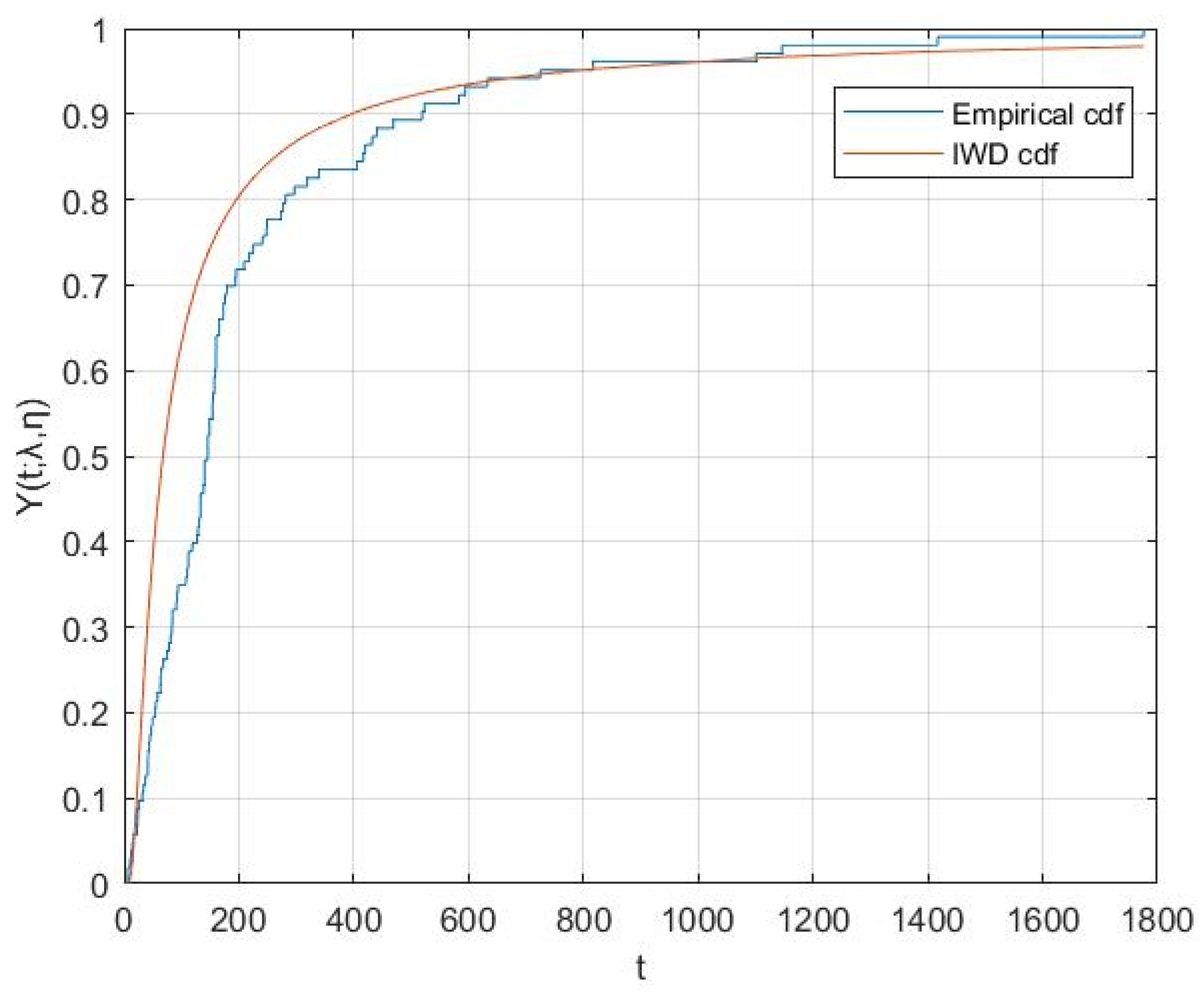
According to the simulation results presented in Section 5, we took the Bayesian estimates of the parameters and reliability under the SE loss function to draw the cumulative distribution function plot. It can be seen in Figure 3 that the cdf of the IWD has a high degree of overlap with the empirical cdf. We can conclude that the IWD has a good fitting effect on this real dataset.
The real dataset was transformed into intuitional fuzzy data by Equations (60) and (61). All the estimates were calculated by MATLAB and are tabulated in Table 4.

7. Conclusions, Limitations, and Future Research

In a real-life scenario, the observed data may be less accurate due to uncontrollable factors, necessitating the use of fuzzy lifetime data for the reliability estimation of the IWD. While fuzzy sets are commonly used for this purpose, they only have one membership degree parameter, resulting in a less precise description of the objective world. In contrast, intuitionistic fuzzy sets can more accurately express uncertainty and fuzziness when dealing with fuzzy information, thereby improving the accuracy and efficiency of fuzzy reasoning. Therefore, this paper extended the probability to intuitionistic fuzzy sets and considered the parameters and reliability estimations for IWD based on intuitionistic fuzzy lifetime data. First, the MLEs were obtained through the EM algorithm. Then, BEs were obtained under the SE and SSE loss functions using the Lindley approximation. Finally, multiple sets of parameters were selected for the Monte Carlo simulation. Based on the simulation results, it was observed that by altering the true values of multiple sets of parameters, the mean square error under the Bayesian estimation was significantly smaller than that under the maximum likelihood estimation. This finding leads to the conclusion that the Bayesian estimation is a more effective approach for estimating parameters and reliability in an intuitionistic fuzzy environment.
Limited by the performance of the computer, we could not compare the performances of more methods during a limited time frame. In addition, there were many types of intuitionistic fuzzy numbers in addition to TraIFNs. We hope to discuss the statistical inference of lifetime distribution based on other types of intuitionistic fuzzy numbers in the future.

Author Contributions

Conceptualization, H.R. and X.H.; methodology, H.R.; software, X.H.; validation, H.R. and X.H.; writing—original draft preparation, X.H.; writing—review and editing, H.R.; funding acquisition, H.R. All authors have read and agreed to the published version of the manuscript.

Funding

This research was funded by the National Natural Science Foundation of China, grant number 71661012.

Data Availability Statement

Not applicable.

Conflicts of Interest

The authors declare no conflict of interest.

References

  1. Yilmaz, A.; Kara, M. Reliability estimation and parameter estimation for inverse Weibull distribution under different loss functions. Kuwait J. Sci. 2022, 49, 1–24. [Google Scholar] [CrossRef]
  2. Chakrabarty, J.B.; Chowdhury, S. Compounded inverse Weibull distributions: Properties, inference and applications. Commun. Stat.-Simul. Comput. 2019, 48, 2012–2033. [Google Scholar] [CrossRef]
  3. Cai, J.; Shi, Y.M.; Zhang, Y.G. Robust Bayesian analysis for parallel system with masked data under inverse Weibull lifetime distribution. Commun. Stat.-Theor. Methods 2020, 49, 1422–1434. [Google Scholar] [CrossRef]
  4. Bi, Q.X.; Gui, W.H. Bayesian and classical estimation of stress-strength reliability for inverse Weibull lifetime models. Algorithms 2017, 10, 71. [Google Scholar] [CrossRef]
  5. Maurya, R.K.; Tripathi, Y.M.; Kayal, T. Reliability Estimation in a Multicomponent Stress-Strength Model Based on Inverse Weibull Distribution. Sankhya B 2022, 84, 364–401. [Google Scholar] [CrossRef]
  6. Majd, A.; Amal, H. Estimation of the stress-strength reliability for the inverse Weibull distribution under adaptive type-II progressive hybrid censoring. PLoS ONE 2022, 17, 0277514–0277536. [Google Scholar]
  7. Krishna, H.; Dube, M.; Garg, R. Estimation of stress strength reliability of inverse Weibull distribution under progressive first failure censoring. Aust. J. Stat. 2019, 48, 14–37. [Google Scholar] [CrossRef]
  8. Yadav, A.S.; Singh, S.K.; Singh, U. Estimation of stress-strength reliability for inverse Weibull distribution under progressive type-II censoring scheme. J. Ind. Prod. Eng. 2018, 35, 48–55. [Google Scholar] [CrossRef]
  9. Yusra, A.T.; Ehab, M.A.; Randa, R.; Ahmed, M.G.; El-Raouf, M.M.A.; Saima, K.K.; Eslam, H.; Bakr, M.E. Statistical inferences for the extended inverse Weibull distribution under progressive type-II censored sample with applications. Alex. Eng. J. 2022, 65, 493–502. [Google Scholar]
  10. Zadeh, L.A. Probability measures of Fuzzy events. J. Math. Anal. Appl. 1968, 23, 421–427. [Google Scholar] [CrossRef]
  11. Li, Z.; Wang, Z.; Song, Y.; Wen, C.F. Information structures in a fuzzy set-valued information system based on granular computing. Int. J. Approx. Reason. 2021, 134, 72–94. [Google Scholar] [CrossRef]
  12. Dang, E.K.F.; Luk, R.; Allan, J. A principled approach using fuzzy set theory for passage-based document retrieval. IEEE Trans. Fuzzy Syst. 2021, 29, 1967–1977. [Google Scholar] [CrossRef]
  13. Jiang, J.W.; Hu, Y.H.; Fang, Y.H.; Zhang, C.; Rui, X.S.; Wang, M. Fault diagnosis method of marine fans based on MTAD and fuzzy entropy. China Mech. Eng. 2022, 33, 1178–1188. [Google Scholar]
  14. Pan, J.S. Research progress on deep learning-based image deblurring. Comput. Sci. 2021, 48, 9–13. [Google Scholar]
  15. Xia, J.N.; Wang, D.J.; Wang, Y.Z.; Jin, Y.C.; Jiang, B. Prostate cancer diagnosis method based on structure adaptive fuzzy neural network. Syst. Eng.-Theor. Pract. 2018, 38, 1331–1342. [Google Scholar]
  16. Taha, T.A.; Salman, A.N. Comparison Different Estimation Method for Reliability Function of Rayleigh Distribution Based on Fuzzy Lifetime Data. Iraqi J. Sci. 2022, 63, 1707–1719. [Google Scholar] [CrossRef]
  17. Rudnei, D.D.C.; Elismar, R.O.; Filip, S. Fuzzy-set approach to invariant idempotent measures. Fuzzy Sets Syst. 2023, 457, 46–65. [Google Scholar]
  18. Hashim, A.N. On the fuzzy reliability estimation for Lomax distribution. AIP Conf. Proc. 2019, 2183, 110002–110011. [Google Scholar]
  19. Neamah, M.W.; Ali, B.K. Fuzzy reliability estimation for frechet distribution by using simulation. Period. Eng. Nat. Sci. 2020, 8, 632–646. [Google Scholar]
  20. Abbas, P.; Gholam, A.P.; Mansour, S. Reliability estimation in Rayleigh distribution based on fuzzy lifetime data. Int. J. Syst. Assur. Eng. 2014, 5, 487–494. [Google Scholar]
  21. Atanassov, K.T. Intuitionistic fuzzy sets. Fuzzy Sets Syst. 1986, 20, 87–96. [Google Scholar] [CrossRef]
  22. Yazdi, M. Risk assessment based on novel intuitionistic fuzzy-hybrid-modified TOPSIS approach. Saf. Sci. 2018, 110, 438–448. [Google Scholar] [CrossRef]
  23. Otay, R.; Ztayi, B.; Onar, S.E.; Kahraman, C. Multi-expert performance evaluation of healthcare institutions using an integrated intuitionistic fuzzy AHP&DEA methodology. Knowl.-Based Syst. 2018, 133, 90–106. [Google Scholar]
  24. Xu, W.; Yu, Y.Y.; Zhang, Q.S. An evaluation method of comprehensive product quality for customer satisfaction based on intuitionistic fuzzy number. Discret. Dyn. Nat. Soc. 2018, 2018, 1–12. [Google Scholar] [CrossRef]
  25. Gohain, B.; Chutia, R.; Dutta, P. Distance measure on intuitionistic fuzzy sets and its application in decision-making, pattern recognition, and clustering problems. Int. J. Intell. Syst. 2022, 37, 2458–2501. [Google Scholar] [CrossRef]
  26. Xu, J.; Ma, Z.; Xu, Z. Novel intuitionistic fuzzy weighted geometric operators for intuitionistic fuzzy multi-attribute decision making. J. Ind. Manag. Optim. 2023, 19, 7196–7220. [Google Scholar] [CrossRef]
  27. Zahra, R.; Ezzatallah, B.J.; Einolah, D. The reliability analysis based on the generalized intuitionistic fuzzy two-parameter Pareto distribution. Soft Comput. 2022, 21, 3095–3113. [Google Scholar]
  28. Ebrahimnejad, A.; Jamkhaneh, E.B. System reliability using generalized intuitionistic fuzzy Rayleigh lifetime distribution. Appl. Appl. Math. 2018, 13, 97–113. [Google Scholar]
  29. Huibert, K. Fuzzy random variables—I. definitions and theorems. Inform. Sci. 1978, 15, 1–29. [Google Scholar]
  30. Zahra, R.; Ezzatallah, B.J.; Einolah, D. Parameters and reliability estimation for the Weibull distribution based on intuitionistic fuzzy lifetime data. Complex Intell. Syst. 2022, 8, 4881–4896. [Google Scholar]
  31. Shu, M.H.; Cheng, C.H.; Chang, J.R. Using intuitionistic fuzzy sets for fault-tree analysis on printed circuit board assembly. Microelectron. Reliab. 2006, 46, 2139–2148. [Google Scholar] [CrossRef]
  32. Wang, J.Q.; Zhang, Z. Programming method of multi-criteria decision-making based on intuitionistic fuzzy number with incomplete certain information. Control Decis. 2008, 23, 1145–1148. [Google Scholar]
  33. Dempster, A.P. Maximum likelihood from incomplete data via the EM algorithm. J. R. Stat. Soc. 1977, 39, 1–38. [Google Scholar]
  34. Singh, S.; Tripathi, Y.M. Estimating the parameters of an inverse Weibull distribution under progressive type-I interval censoring. Stat. Pap. 2018, 59, 21–56. [Google Scholar] [CrossRef]
  35. Kurniawan, A.; Avicena, N.; Ana, E. Estimation of the shape parameter of Weibull distribution based on type II censored data using EM algorithm. AIP Conf. Proc. 2020, 2264, 030011–030020. [Google Scholar]
  36. Barde, S.; Ko, Y.M.; Shin, H. General EM algorithm for fitting non-monotone hazard functions from truncated and censored observations. Oper. Res. Lett. 2022, 50, 476–483. [Google Scholar] [CrossRef]
  37. Pal, S. A simplified stochastic EM algorithm for cure rate model with negative binomial competing risks: An application to breast cancer data. Stat. Med. 2021, 40, 6387–6409. [Google Scholar] [CrossRef]
  38. Fu, E.; Heckman, N. Model-based curve registration via stochastic approximation EM algorithm. Comput. Stat. Data An. 2019, 131, 159–175. [Google Scholar] [CrossRef]
  39. Wang, Z.G.; Liu, W.C. Stochastic reserving using policyholder information via EM algorithm. Appl. Math. Model. 2022, 112, 199–214. [Google Scholar] [CrossRef]
  40. Lachos, V.H.; Prates, M.O.; Dey, D.K. Heckman selection-t model: Parameter estimation via the EM-algorithm. J. Multivar. Anal. 2021, 184, 104737–104755. [Google Scholar] [CrossRef]
  41. Jia, X.; Cheng, Z.J.; Guo, B. Reliability evaluation for products based on entropy and Bayes theory. Syst. Eng. Theory Pract. 2020, 40, 1918–1926. [Google Scholar]
  42. Li, D.W.; Wang, G.D.; Li, Y.Z. Qualification test risk analysis of binomial equipment based on Bayes theory. J. Aerosp. Power 2021, 36, 157–166. [Google Scholar]
  43. Wang, C.Y.; Huang, X.J. Comparison of Bayesian estimation of the scale parameter for Log gamma distribution under Linex loss function and compound Linex loss function. Math. Appl. 2018, 31, 384–391. [Google Scholar]
  44. Kundu, D.; Mitra, D. Bayesian inference of Weibull distribution based on left truncated and right censored data. Comput. Stat. Data An. 2016, 99, 38–50. [Google Scholar] [CrossRef]
  45. Xu, B.; Wang, D.H.; Wang, R.T. Estimator of scale parameter in a subclass of the exponential family under symmetric entropy loss. Northeast Math. J. 2008, 24, 447–457. [Google Scholar]
  46. Song, L.X.; Chen, Y.S.; Xu, J.M. Bayesian estimation of Poisson distribution parameter under scale squared error loss function. J. Lanzhou Univ. Tech. 2008, 34, 152–154. [Google Scholar]
  47. Usta, I. Bayesian estimation for geometric process with the Weibull distribution. Commun. Stat.-Simul. Comput. 2022, 1–27. [Google Scholar] [CrossRef]
  48. González, R.G.; Colubi, A.; Ángeles, G.M. A fuzzy representation of random variables: An operational tool in exploratory analysis and hypothesis testing. Comput. Stat. Data Anal. 2006, 51, 163–176. [Google Scholar] [CrossRef]
  49. Efron, B. Logistic regression, survival analysis, and the Kaplan-Meier curve. J. Am. Stat. Assoc. 1988, 83, 414–425. [Google Scholar] [CrossRef]
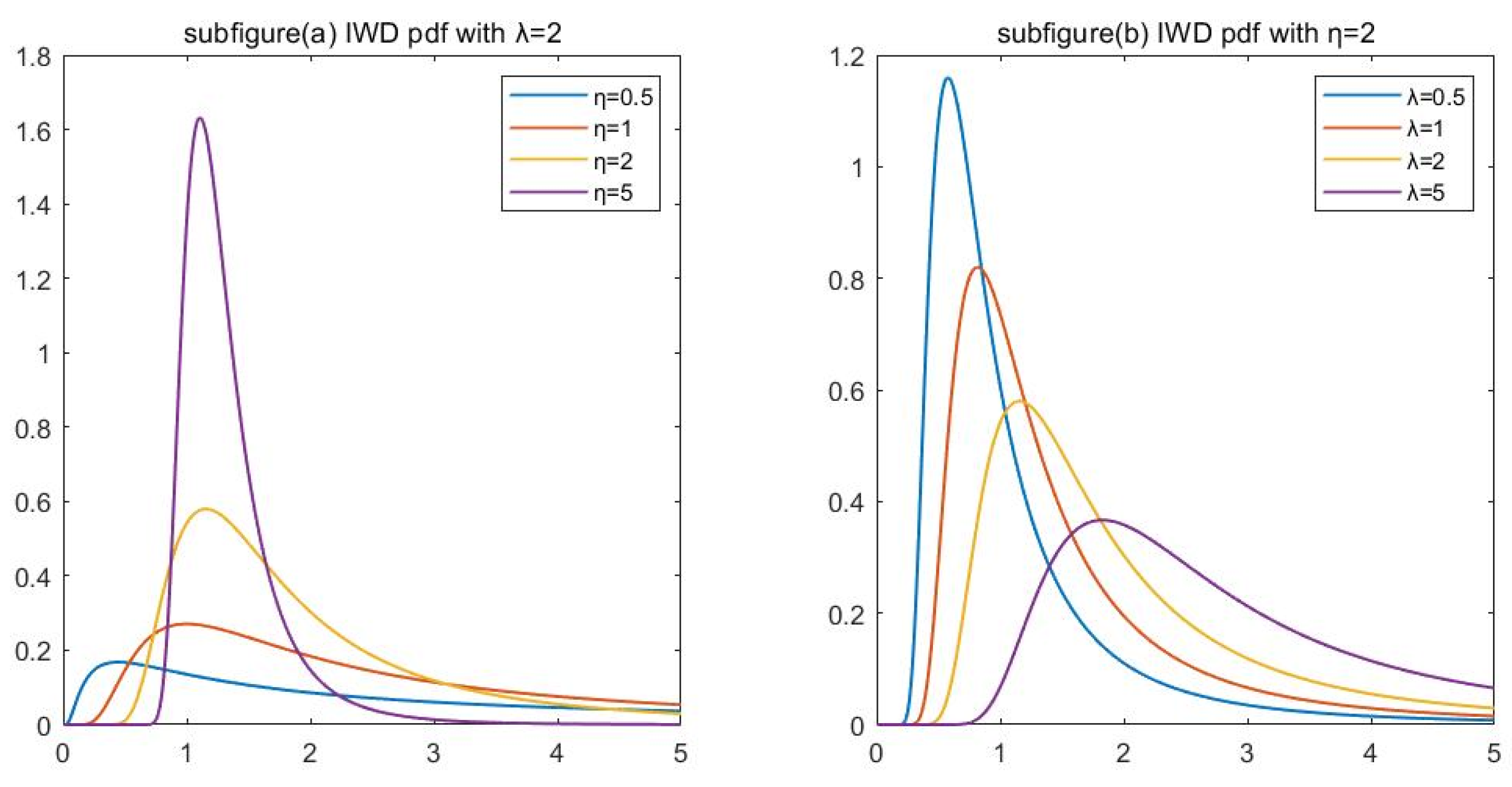
Figure 1. The pdf of IWD.
Axioms 12 00838 g001
Figure 2. The risk function of IWD.
Axioms 12 00838 g002
Figure 3. Empirical and IWD cdf values.
Axioms 12 00838 g003
Table 1. The MSEs of λ and η .
n λ r e a l η r e a l MSE
λ ^ M L λ ^ S E λ ^ S S E η ^ M L η ^ S E η ^ S S E
20510.6252 0.5126 0.2208 0.1247 0.0171 0.0056
840.8302 0.7005 0.4867 0.6479 0.2369 0.1875
230.8011 0.6801 0.1644 0.8141 0.4975 0.1810
50510.4900 0.0584 0.0543 0.0458 0.0009 9.94 × 10⁻⁴
840.6842 0.5550 0.4786 0.3718 0.0762 0.0530
230.6195 0.0048 0.0053 0.5094 0.1396 0.0638
100510.1330 0.0143 0.0165 0.0358 0.0002 0.0003
840.2717 0.1148 0.1819 0.1138 0.0150 0.0154
230.3339 0.0003 0.0013 0.1838 0.0218 0.0213
200510.0525 0.0034 0.0044 0.0217 4.64 × 10−56.51 × 10−5
840.0914 0.0562 0.0602 0.0454 0.0033 0.0040
230.1020 0.0001 0.0004 0.0840 0.0039 0.0052
300510.0240 0.0016 0.0021 0.0214 2.12 × 10−52.96 × 10−5
840.0840 0.0253 0.0295 0.0096 0.0015 0.0019
230.0863 5.31 × 10−50.0002 0.0472 0.0017 0.0024
400510.0093 0.0009 0.0012 0.0184 1.24 × 10−51.72 × 10−5
840.0692 0.0142 0.0174 0.0016 8.25 × 10−40.0011
230.0691 2.21 × 10−59.63 × 10−50.0112 9.55 × 10−40.0014
500510.0087 0.00060.0008 0.0168 7.89 × 10−61.11 × 10−5
840.0590 0.00920.0115 0.0008 5.50 × 10−47.24 × 10−4
230.0489 1.27 × 10−55.98 × 10−50.0093 6.39 × 10−49.28 × 10−4
Table 2. MSEs and estimates of R ( t ) .
n λ r e a l η r e a l R ( t ) EstimatesMSE
R ^ M L ( t ) R ^ S E ( t ) R ^ S S E ( t ) R ^ M L ( t ) R ^ S E ( t ) R ^ S S E ( t )
20510.91790.95000.89840.92860.0024 8.98 × 10−43.21 × 10−3
840.39350.40890.39730.34650.0185 8.60 × 10−32.80 × 10−3
230.22120.28260.30030.27980.0083 8.23 × 10−31.82 × 10−2
50510.91790.94830.91220.96210.0011 6.48 × 10−58.72 × 10−5
840.39350.38720.40860.38250.0048 8.11 × 10−45.79 × 10−4
230.22120.17440.26040.23730.0044 5.80 × 10−37.91 × 10−2
100510.91790.92620.91460.91430.0006 1.32 × 10−52.04 × 10−5
840.39350.38910.40350.38850.0029 5.51 × 10−52.55 × 10−5
230.22120.28190.24550.23120.0020 4.32 × 10−43.43 × 10−4
200510.91790.92130.91640.91630.0002 2.69 × 10−64.52 × 10−6
840.39350.33510.39330.38780.0012 8.66 × 10−65.45 × 10−6
230.22120.17830.23310.22510.0013 5.95 × 10−58.19 × 10−6
300510.91790.93990.91690.91680.0002 1.46 × 10−62.23 × 10−6
840.39350.40960.39310.39010.0008 3.82 × 10−62.18 × 10−6
230.22120.25800.22600.22350.0009 2.54 × 10−53.78 × 10−6
400510.91790.92300.91720.91710.0001 1.25 × 10−61.63 × 10−6
840.39350.38260. 39450.39170.0008 2.05 × 10−61.05 × 10−6
230.22120.16640.22520.22280.0007 1.38 × 10−51.95 × 10−6
500510.91790.93930.91720.91710.0001 5.02 × 10−77.84 × 10−7
840.39350.37370.39470.39210.0006 1.40 × 10−66.87 × 10−7
230.22120.20480.22360.22170.0007 9.22 × 10−61.38 × 10−6
Table 3. Real dataset.
6.53710.4212.214.4816.122.723.5623.7425.87
31.98343741.3541.55424345.2847.3849.4
53.6255.4658.366363.476468.4674.4778.2681
838484919294108110112112
119127129130133133133139140140
140146146146149149154154155157
157159160160160160165165173173
176179194195209218225241248249
273277281297319339405417420432
4404695195235835946337258171101
114614171776
Table 4. Real dataset estimates with t = 49.4 .
λ ^ η ^ R ^ ( t )
MLESESSEMLESESSEMLESESSE
64.617167.714067.76300.80001.08861.08850.94230.62050.6170
Disclaimer/Publisher’s Note: The statements, opinions and data contained in all publications are solely those of the individual author(s) and contributor(s) and not of MDPI and/or the editor(s). MDPI and/or the editor(s) disclaim responsibility for any injury to people or property resulting from any ideas, methods, instructions or products referred to in the content.