A Flexible Dispersed Count Model Based on Bernoulli Poisson–Lindley Convolution and Its Regression Model

Abstract

Count data are encountered in real-life dealings. More understanding of such data and the extraction of important information about the data require some statistical analysis or modeling. One innovative technique to increase the modeling flexibility of well-known distributions is to use the convolution of random variables. This study examines the distribution that results from adding two independent random variables, one with the Bernoulli distribution and the other with the Poisson–Lindley distribution. The considered distribution is named as the two-parameter Bernoulli–Poisson–Lindley distribution. Many of its statistical properties are investigated, such as moments, survival and hazard rate functions, mode, dispersion behavior, mean deviation about the mean, and parameter inference based on the maximum likelihood method. To evaluate the effectiveness of the bias and mean square error of the produced estimates, a simulation exercise is carried out. Then, applications to two practical data sets are given. Finally, we construct a flexible count data regression model based on the proposed distribution with two practical examples.

1. Introduction

In recent decades, count data analysis has drawn interest. There are many count data sets in practical as well as theoretical domains, including medicine, sports, engineering, finance, insurance, etc. (see [1]). However, we are unable to use methodologies or typical standard probability distributions to analyze them. Building adaptable models has attracted a lot of interest from statisticians and applied scientists in order to improve the modeling of count data. Therefore, it is critical to create models that are superior to standard distributions in order to successfully investigate real-world data and its attributes.

Recently, for the purpose of modeling count data, several models have evolved. The use of conventional discrete distributions as models for dependability, hazard rates, counts, etc., is limited. The widespread parametric models for analyzing such data are the Poisson, geometric, and negative binomial (NB) models (see [2]). The Poisson regression model is the most common model for modeling count data, but an obstacle arises: there is a fact that they may exhibit over- or under-dispersion, which is when a count’s conditional variance is greater or less than its conditional mean (see [3]). In these cases, the Poisson model’s mean–variance relationship is a well-known drawback. This has led to the introduction of various Poisson distribution types (see [4,5]). A traditional way of overcoming over-dispersion is to allow the single parameter of the Poisson distribution to be a random variable following a given distribution. This is also known as the compounding method, and the idea was first proposed in [6]. The resultant compound distributions are also termed as mixture distributions. One such famous mixture distribution is the negative binomial distribution, obtained by mixing the Poisson distribution with a gamma distribution. In real-world count modeling applications, the negative binomial distribution with an additional dispersion parameter is widely accepted as a solution to the over-dispersion issue.

As a result, various discrete distributions based on widely used continuous distributions for reliability, hazard rates, etc., have been developed. The discrete Weibull distribution is the most well-liked of these. It was introduced in [7,8,9]. Since then, numerous applications have been made. There are many other recently constructed distributions with continuous analogues. The author in [10] introduced the discrete gamma distribution, which has received significant attention for applications in the areas of molecular biology and evolution. Discrete analogues of the continuous Burr and Pareto distributions were constructed in [11]. On the other hand, the authors in [12] introduced a discrete analogue of the continuous inverse Weibull distribution. The discrete Lindley distribution was proposed in [13].

There are so many models for studying over-dispersion, while only a few models are there to deal with under-dispersion, because over-dispersion exists more frequently (see [14]).

Various extensions and generalizations of the Poisson distributions were developed for both over-dispersed and under-dispersed count data in the literature over the last decade. The authors in [15] proposed the generalized Poisson (GP) regression model, whereas those of [16] introduced the Conway–Maxwell–Poisson (COM–Poisson) model. The COM–Poisson regression model was also created. The authors in [17] invented the Poisson–Tweedie regression model.

Each of the aforementioned models has some drawbacks. For instance, the GP model’s range must be truncated in order to achieve under-dispersion, with the level of truncation depending on the actual model parameters. The issue is that because of the range’s shortening, the probabilities no longer add up to 1. The convolutions (sum and difference) of two independent random variables are a clever way of broadening the modeling possibilities of well-known distributions.

The author in [18] proposed the discrete Poisson–Lindley distribution, a compound Poisson distribution obtained by compounding the Poisson distribution with the Lindley distribution. The authors in [19] introduced an efficient regression model for under-dispersed count data based on the Bernoulli–Poisson convolution (BerPoi) for under-dispersed count data. In it, the response variable is distributed according to the BerPoi distribution using a specific parameterization indexed by mean and dispersion parameters.

In this paper, we introduce a distribution generated from the sum of two independent random variables, one with the Bernoulli distribution and the other with the Poisson–Lindley distribution. The resulting distribution is known as the Bernoulli–Poisson–Lindley (BPL) distribution. One of its key advantages is that it is suitable for modeling both under-dispersed and over-dispersed count data, unlike the Poisson distribution. Furthermore, it has only two parameters, which reduces the complexity of the simulation study, unlike some Poisson generalizations with three parameters. Moreover, it has an increasing hazard rate, making it appropriate for modeling equipment wear and tear or ageing processes. The proposed model is appropriate for regression modeling since its moments may be retrieved in closed form.

The remaining sections of the paper are organized as follows: Section 2 presents the BPL distribution. Section 3 discusses the statistical properties of this distribution. Section 4 introduces the parameter estimation using the maximum likelihood method, and its performance is assessed via a simulation study. The new model is shown to perform at least as well as other recently proposed two-parameter discrete models, and the conventional one-parameter discrete models using two real data sets are analyzed in Section 5. In Section 6, a regression model is developed. Finally, several key takeaways are outlined in Section 7.

2. Bernoulli-Poisson-Lindley Distribution

The BPL distribution is obtained by the distribution of the sum of two independent random variables, one with the Bernoulli distribution, and the other with the Poisson–Lindley distribution.

The result below presents a simple expression of the corresponding probability mass function (pmf).

Proposition 1. 

The pmf of the BPL distribution with parameters α and θ can be expressed as

$$p(x,\alpha ,\theta )=\left\{\begin{array}{cc}{\displaystyle \frac{(1-\alpha ){\theta }^2(\theta +2)}{{(\theta +1)}^3}}\hfill & ifx=0\hfill \\ {\displaystyle \frac{{\theta }^2\left[(1+\alpha \theta )(x+\theta +1)+(1-\alpha )\right]}{{(\theta +1)}^{x+3}}}\hfill & ifx=1,2,3,\dots \hfill \end{array}\right.$$

(1)

Proof. 

Let $X_1$ and $X_2$ be two independent random variables, with $X_1$ following the Bernoulli distribution with parameter $0<\alpha <1$, i.e., $P(X_1=0)=1-\alpha$ and $P(X_1=1)=\alpha$ and $X_2$ following the Poisson–Lindley distribution with parameter $\theta >0$, i.e., $P(X_2=x)={\displaystyle \frac{{\theta }^2(x+\theta +2)}{{(\theta +1)}^{x+3}}}$ with $x=0,1,2,3,\dots$ Then, by the definition, the BPL distribution is the distribution of $X=X_1+X_2$. Let us now determine its pmf. For any $x=0,1,\dots$, we have

$$\begin{array}{cc}\hfill p(x,\alpha ,\theta )& =P(X=x)=P(X_1+X_2=x)\hfill \\ \hfill & =P(X_1=0)P(X_2=x)+P(X_1=1)P(X_2=x-1).\hfill \end{array}$$

In particular, for $x=0$, we have

$$\begin{array}{cc}\hfill p(x,\alpha ,\theta )& =P(X_1=0)P(X_2=0)={\displaystyle \frac{(1-\alpha ){\theta }^2(\theta +2)}{{(\theta +1)}^3}}.\hfill \end{array}$$

For $x=1,2,\dots$, we have

$$\begin{array}{cc}\hfill p(x,\alpha ,\theta )& =P(X=x)\hfill \\ \hfill & =(1-\alpha ){\displaystyle \frac{{\theta }^2(x+\theta +2)}{{(\theta +1)}^{x+3}}}+\alpha {\displaystyle \frac{{\theta }^2(x-1+\theta +2)}{{(\theta +1)}^{x-1+3}}}\hfill \\ \hfill & ={\displaystyle \frac{{\theta }^2}{{(\theta +1)}^{x+3}}}[\alpha (x+\theta +1)(\theta +1)+(1-\alpha )(x+2+\theta )]\hfill \\ \hfill & ={\displaystyle \frac{{\theta }^2}{{(\theta +1)}^{x+3}}}[\alpha \theta (x+\theta +1)+\alpha (x+\theta +1)+(1-\alpha )(x+\theta +1+1)]\hfill \\ \hfill & ={\displaystyle \frac{{\theta }^2}{{(\theta +1)}^{x+3}}}[\alpha \theta (x+\theta +1)+\alpha (x+\theta +1)+(1-\alpha )(x+\theta +1)+(1-\alpha )]\hfill \\ \hfill & ={\displaystyle \frac{{\theta }^2}{{(\theta +1)}^{x+3}}}[(1+\alpha \theta )(x+\theta +1)+(1-\alpha )].\hfill \end{array}$$

This ends the proof of Proposition 1.   □

Remark 1. 

When $\alpha \to 0$, the Poisson–Lindley distribution is included in the BPL distribution as a special case.

Proposition 2. 

The cumulative density function (cdf) of the BPL distribution can be expressed as, for any integer x,

$$F(x,\alpha ,\theta )=1+{\displaystyle \frac{[-1-\theta (3+x+\theta +x\alpha \theta +\alpha \theta (2+\theta )\left)\right]}{{(1+\theta )}^{x+3}}},x=0,1,2,\dots$$

(2)

Proof. 

It follows from the geometric series expansions and some algebra, that

$$\begin{array}{cc}\hfill F(x,\alpha ,\theta )& =\sum _{k=0}^{x}p(k,\alpha ,\theta )\hfill \\ \hfill & ={\displaystyle \frac{{\theta }^2(1-\alpha )(\theta +2)}{{(\theta +1)}^3}}+\sum _{k=1}^x{\displaystyle \frac{{\theta }^2\left[\left[\right(1+\alpha \theta \left)\right(k+\theta +1\left)\right]+(1-\alpha )\right]}{{(\theta +1)}^{k+3}}}\hfill \\ \hfill & =1+{\displaystyle \frac{[-1-\theta (3+x+\theta +x\alpha \theta +\alpha \theta (2+\theta )\left)\right]}{{(1+\theta )}^{x+3}}}.\hfill \end{array}$$

This ends the proof of Proposition 2.    □

The corresponding survival function is given by

$$S(x,\alpha ,\theta )={\displaystyle \frac{1+\theta [3+x+\theta +x\alpha \theta +\alpha \theta (2+\theta \left)\right]}{{(1+\theta )}^{x+3}}},x=0,1,2,\dots$$

(3)

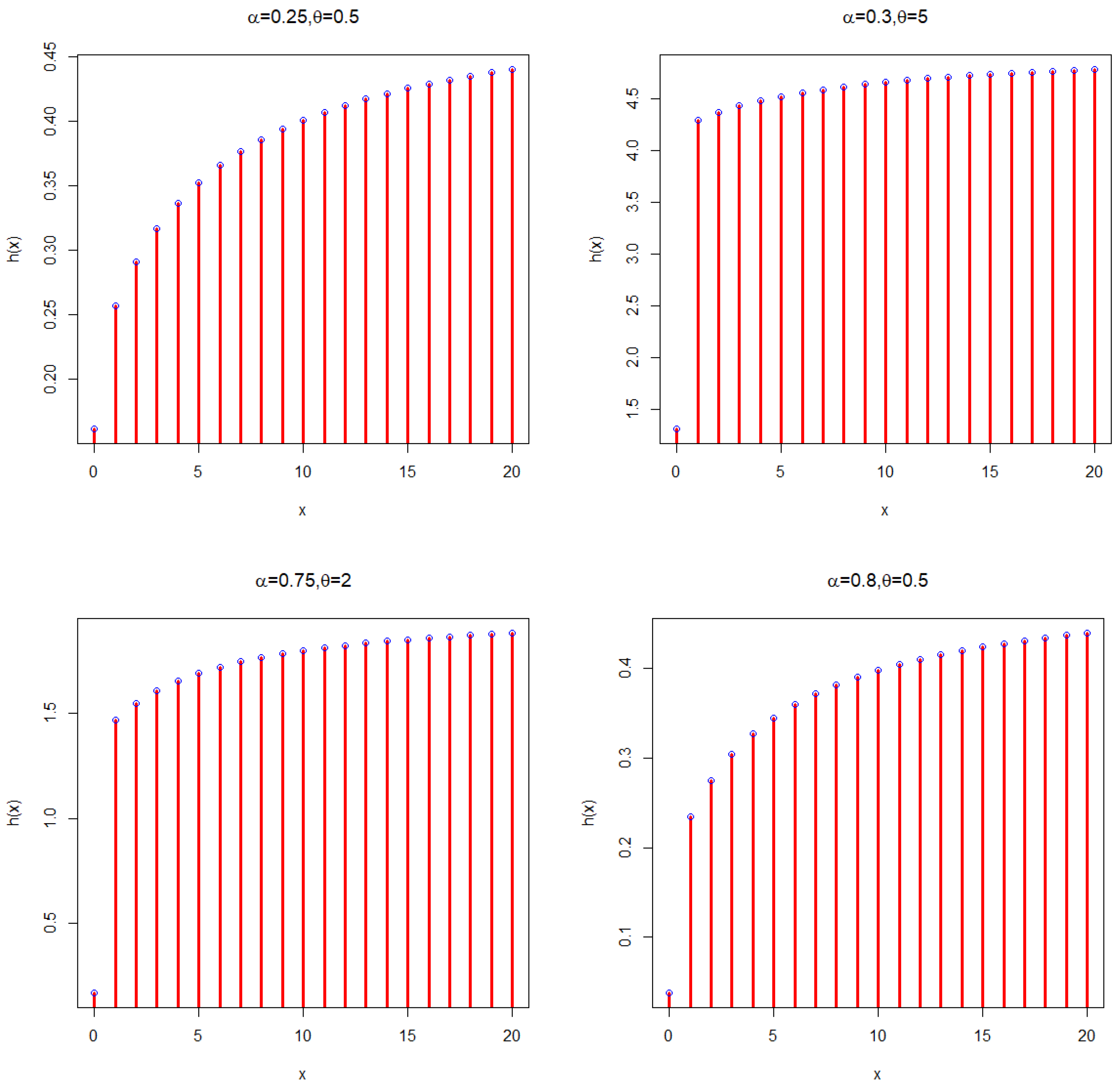
The hazard rate function (hrf) of the BPL distribution is obtained as

$$h(x,\alpha ,\theta )=\left\{\begin{array}{cc}{\displaystyle \frac{(1-\alpha ){\theta }^2(\theta +2)}{1+\theta [3+\theta +\alpha \theta (2+\theta \left)\right]}}\hfill & ifx=0\hfill \\ {\displaystyle \frac{{\theta }^2[1-\alpha +(1+x+\theta )(1+\alpha \theta )]}{1+\theta [3+x+\theta +x\alpha \theta +\alpha \theta (2+\theta \left)\right]}}\hfill & ifx=1,2,3,\dots \hfill \end{array}\right.$$

(4)

  Figure 1 shows the different shapes of the pmf. It clearly indicates that the BPL distribution is positively skewed, unimodal and as $\theta$ goes larger, the mass concentrates more on values closer to 0 than at higher values. Figure 2 also presents different shapes of the cdf.

Figure 3 presents different shapes of the hrf, indicating that the BPL distribution exhibits increasing hazard rates with respect to both $\alpha$ and $\theta$.

3. Statistical Properties

3.1. Mode

We now provide some theory to the observation of the mode of the BPL distribution made in Figure 1.

Proposition 3. 

Let X be a random variable following the BPL distribution. Then, the mode of X, denoted by $x_m$, exists in {0,1, 2, …}, and satisfies

$$\begin{array}{c}\hfill -1+{\displaystyle \frac{1}{\theta }}-\theta +{\displaystyle \frac{2+\alpha }{1+\alpha \theta }}\le x_m\le {\displaystyle \frac{1}{\theta }}-\theta +{\displaystyle \frac{\alpha -1}{1+\alpha \theta }},\end{array}$$

(5)

with $x_m=0$ if the upper bound is non-positive.

Proof. 

By the definition of the mode, it corresponds to the integer $x=x_m$ for which $p(x,\alpha ,\theta )$ has the greatest value, where we recall that

$$\begin{array}{c}\hfill p(x,\alpha ,\theta )=\left\{\begin{array}{cc}(1-\alpha ){\theta }^2{\displaystyle \frac{(\theta +2)}{{(\theta +1)}^3}}\hfill & ifx=0\hfill \\ {\displaystyle \frac{{\theta }^2}{{(\theta +1)}^{x+3}}}\left[(1+\alpha \theta )(x+\theta +1)+(1-\alpha )\right]\hfill & ifx=1,2,3,\dots \hfill \end{array}\right.\end{array}$$

(6)

To reach our aim, we need to solve $p(x_m,\alpha ,\theta )\ge p(x_m-1,\alpha ,\theta )$ and $p(x_m,\alpha ,\theta )\ge p(x_m+1,\alpha ,\theta )$. Obviously, $p(x_m,\alpha ,\theta )\ge p(x_m-1,\alpha ,\theta )$ implies that

$$\begin{array}{c}\hfill x_m\le {\displaystyle \frac{1}{\theta }}-\theta +{\displaystyle \frac{\alpha -1}{1+\alpha \theta }}.\end{array}$$

(7)

Furthermore, $p(x_m,\alpha ,\theta )\ge p(x_m+1,\alpha ,\theta )$ implies that

$$\begin{array}{c}\hfill x_m\ge -1+{\displaystyle \frac{1}{\theta }}-\theta +{\displaystyle \frac{2+\alpha }{1+\alpha \theta }}.\end{array}$$

(8)

By combining Equations (7) and (8), we obtain Equation (5), hence, the proof of Proposition 3.   □

3.2. Moments, Skewness, and Kurtosis

Hereafter, let X be a random variable following the BPL distribution. Then, after some algebraic developments, the probability generating function of X is given by

$$\begin{array}{cc}\hfill P\left(s\right)& =E\left(s^X\right)={\displaystyle \frac{[1+(-1+s)\alpha ]{\theta }^2(2-s+\theta )}{(1+\theta ){(1-s+\theta )}^2}},\hfill \end{array}$$

for $s<\theta +1$.

The moment-generating function of X can be obtained by replacing s by $e^t$, for $t<log(\theta +1)$, which gives

$$\begin{array}{cc}\hfill M\left(t\right)& =E\left(e^{tX}\right)={\displaystyle \frac{[1+(-1+e^t)\alpha ]{\theta }^2(2-e^t+\theta )}{(1+\theta ){(1-e^t+\theta )}^2}}.\hfill \end{array}$$

Basically, the r-th moment about the origin of X is derived as

$$\begin{array}{cc}\hfill E\left(X^r\right)& =\sum _{x=0}^{\infty }{x}^{r}p(x,\alpha ,\theta )=\sum _{x=1}^{\infty }{x}^r{\displaystyle \frac{{\theta }^2}{{(\theta +1)}^{x+3}}}\left[(1+\alpha \theta )(x+\theta +1)+(1-\alpha )\right]\hfill \end{array}.$$

Thus, after an intense use of the geometric series formulas (see Appendix A), the first four moments of X are

$$\begin{array}{cc}\hfill E\left(X\right)& =\alpha +{\displaystyle \frac{2+\theta }{\theta (\theta +1)}},\hfill \\ \hfill E\left(X^2\right)& ={\displaystyle \frac{6+\theta [4+\theta +\alpha (4+\theta (3+\theta )\left)\right]}{{\theta }^2(1+\theta )}},\hfill \\ \hfill E\left(X^3\right)& ={\displaystyle \frac{24+\theta \left[24+\theta (8+\theta )+\alpha (3+\theta )(6+\theta (4+\theta \left)\right)\right]}{{\theta }^3(1+\theta )}},\hfill \end{array}$$

and

$$\begin{array}{cc}\hfill E\left(X^4\right)& =\frac{120+\theta \left[168+\theta [78+\theta (16+\theta \left)\right]+\alpha [96+\theta (132+\theta [64+\theta (15+\theta \left)\right]\left)\right]\right]}{{\theta }^4(1+\theta )}.\hfill \end{array}$$

Now, the variance of X is calculated as

$$\begin{array}{cc}\hfill V\left(X\right)& =E\left(X^2\right)-{\left[E\left(X\right)\right]}^2={\displaystyle \frac{2+\theta [6+\theta (4+\theta +(1-\alpha )\alpha {(1+\theta )}^2)]}{{\theta }^2{(1+\theta )}^2}}.\hfill \end{array}$$

Figure 4 presents the plots of the variance of X for different values of the parameters $\alpha$ and $\theta$. We see that the variance decreases when $\alpha$ is fixed and $\theta$ increases.

On the other hand, based on the first four moments of X, the skewness of X is

$$Skewness\left(X\right)={\displaystyle \frac{{[4+\theta (18+\theta [32+\theta (22+\alpha {(1+\theta )}^3-3{\alpha }^2{(1+\theta )}^3+2{\alpha }^3{(1+\theta )}^3+\theta (7+\theta ))])]}^2}{{[2-\theta (6-\theta [4+\theta +(1-\alpha )\alpha (1+{\theta }^2)])]}^3}}.$$

Furthermore, the kurtosis of X is

$$\begin{array}{cc}\hfill Kurtosis\left(X\right)& ={\displaystyle \frac{1}{{[-2+\theta (-6+\theta [-4-\theta -(1-\alpha )\alpha {(1+\theta )}^2])]}^2}}[24+\theta (144+\theta [338+\hfill \\ \hfill & 6{\alpha }^3{\theta }^2{(1+\theta )}^4-3{\alpha }^4{\theta }^2{(1+\theta )}^4+\alpha {(1+\theta )}^2[12+\theta (4+\theta )(9+\theta [4+\theta ])]+\hfill \\ \hfill & \theta [406+\theta (258+\theta (87+\theta [15+\theta \left]\right)\left)\right]\hfill \\ \hfill & -2{\alpha }^2{(1+\theta )}^2[6+\theta (18+\theta [14+\theta (7+2\theta )])]\left]\right)].\hfill \end{array}$$

Figure 5 presents the plots of the skewness and kurtosis of X, respectively. From these plots, when the value of $\alpha$ is held constant, and $\theta$ increases, a significant effect on both the skewness and kurtosis is observed. Furthermore, when $\theta$ increases, the BPL distribution is rightly skewed and leptokurtic.

3.3. Dispersion Index and Coefficient of Variation

In this section, we discuss the dispersion index (DI) and coefficient of variation (CV) associated with the BPL distribution. The CV of X is obtained as

$$\begin{array}{c}\hfill CV\left(X\right)={\displaystyle \frac{\sqrt{2+\theta [6+\theta (4+\theta +(1-\alpha )\alpha {(1+\theta )}^2)]}}{2+\theta +\alpha \theta (\theta +1)}}.\end{array}$$

The DI of X is given by

$$\begin{array}{c}\hfill DI\left(X\right)=1+{\displaystyle \frac{1}{\theta }}+\frac{1}{1+\theta }-\left(\alpha +\frac{1-\alpha +\alpha \theta }{2+\theta (1+\alpha +\alpha \theta )}\right).\end{array}$$

Clearly, $DI\left(X\right)$ is greater than 1 when $\theta$ tends to 0, and less than 1 when $\theta$ tends to ∞. Thus, the BPL distribution has under- or over-dispersed properties.

Numerical values for some moment measures, such as mean, variance, DI, skewness, and kurtosis for the BPL distribution for different sets of parameter values are given in

Table 1. Numerical values for some moment measures associated with the BPL distribution for $\alpha$ = 0.1 and different values of $\theta$.

Measures	$\mathit{\theta }$
	0.1	10	50	99	999
Mean	19.1909	0.2091	0.1204	0.1102	0.1010
Variance	218.3545	0.2108	0.1108	0.1003	0.0910
DI	11.3780	1.0083	0.9204	0.9102	0.9010
Skewness	2.0459	5.1086	6.4470	6.7468	7.0719
Kurtosis	6.0496	8.5888	8.2779	8.2024	8.1209

and

Table 2. Numerical values for some moment measures associated with the BPL distribution for $\alpha$ = 0.3 and different values of $\theta$.

Measures	$\mathit{\theta }$
	0.1	10	50	99	999
Mean	19.3909	0.4091	0.3204	0.3102	0.3010
Variance	218.4745	0.3309	0.2308	0.2203	0.2110
DI	11.2669	0.8087	0.7204	0.7102	0.7010
Skewness	2.0426	1.4711	0.9079	0.8355	0.7692
Kurtosis	6.0462	4.3926	2.4144	2.1001	1.7964

. It can be observed that the mean and variance decrease as $\theta$ tends to ∞ for fixed values of $\alpha$.

3.4. Mean Deviation about the Mean

The mean deviation (MD) about the mean measures the amount of scatter in a population. Let $\mu$ be the mean of the BPL distribution, i.e., $\mu =E\left(X\right)=\alpha +{\displaystyle \frac{2+\theta }{\theta (\theta +1)}}.$ Then the MD about the mean is defined as $MD\left(X\right)=E\left(|X-\mu |\right)$, and can be calculated as

$$\begin{array}{cc}\hfill MD\left(X\right)& =\sum _{x=0}^{\infty }|x-\mu |p(x,\alpha ,\theta )\hfill \\ \hfill & =\mu p(0,\alpha ,\theta )+\sum _{x=1}^{\lfloor \mu \rfloor }(\mu -x)p(x,\alpha ,\theta )+\sum _{x=\lfloor \mu \rfloor +1}^{\infty }(x-\mu )p(x,\alpha ,\theta )\hfill \\ \hfill & ={\displaystyle \frac{{(1+\theta )}^{-3-\lfloor \mu \rfloor }}{\theta }}\left[2{(1+\theta )}^2\right[2+\theta (1+\alpha +\alpha \theta )]-2\theta (1+\theta [3+\theta +\alpha \theta (2+\theta )])\mu \hfill \\ \hfill & -{(1+\theta )}^{2+\lfloor \mu \rfloor }[2+\theta (1+\alpha +\alpha \theta -(1+\theta )\mu )]\hfill \\ \hfill & +2\theta \lfloor \mu \rfloor (2+\theta [4+\alpha +\theta +\alpha \theta (3+\theta -\mu )-\mu ]+\theta (1+\alpha \theta )\lfloor \mu \rfloor )],\hfill \end{array}$$

where $\lfloor \mu \rfloor$ is the greatest integer less than or equal to $\mu$.

Figure 6 shows the plot of the MD about the mean of X. From this plot, we observe that when $\theta$ increases, the values of the MD about the mean decrease.

4. Parameter Estimation

Parameter estimation is an important step toward a deeper understanding of the process. The classical method of estimation, the maximum likelihood (ML) method, is used here to estimate the parameters. Let $X_1,X_2,\dots ,X_n$ be a random sample of size n from a BPL distribution with unknown parameters $\alpha$ and $\theta$. Let $x_1,\dots ,x_n$ be the n observed values. Let y be the number of $x_i$ taking the value 0 and $(n-y)$ of $x_i$’s are taking the nonzero values. The log-likelihood function is given by

$$\begin{array}{cc}\hfill logL(\alpha ,\theta )& =ylog(1-\alpha )+2ylog\theta +ylog(\theta +2)-3ylog(\theta +1)+2(n-y)log\theta \hfill \\ \hfill & -3(n-y)log(1+\theta )\hfill \\ \hfill & +\sum _{i=1,x_i\ne 0}^{n-y}\left\{log[(1+\alpha \theta )(1+\theta +x_i)+(1-\alpha )]-x_{i}log(\theta +1)\right\}.\hfill \end{array}$$

The maximum likelihood estimates (MLEs) of $\alpha$ and $\theta$ are the values that maximize $logL(\alpha ,\theta )$. They are denoted as $\widehat{\alpha }$ and $\widehat{\theta }$, respectively. The partial derivatives of $logL(\alpha ,\theta )$ with respect to each parameter are the following:

$$\begin{array}{cc}\hfill \frac{\partial }{\partial \alpha }logL(\alpha ,\theta )& =\sum _{i=1}^{n-y}\left\{\frac{\theta (1+x_i+\theta )-1}{(1+\alpha \theta )(1+x_i+\theta )+(1-\alpha )}\right\}-\frac{y}{1-\alpha },\hfill \\ \hfill \frac{\partial }{\partial \theta }logL(\alpha ,\theta )& =\sum _{i=1}^{n-y}\left\{\frac{(1+\alpha \theta )+(1+x_i+\theta )\alpha }{(1+\alpha \theta )(1+x_i+\theta )+(1-\alpha )}\right\}-\frac{n(3+\overline{x})}{\theta +1}+\frac{y}{\theta +2}+\frac{2n}{\theta }.\hfill \end{array}$$

In order to obtain the MLEs, note that the above system of equations set to zero contains non-linear equations and does not have an explicit solution. Consequently, the system must be solved numerically, for example, using the statistical programming language R (see Appendix A).

Simulation Study

In this section, a brief simulation study is performed to evaluate the asymptotic behavior of the MLEs for different parametric combinations. Here the iteration is carried out for different sample sizes (50, 100, 200, 500, 1000) and $N=1000$ replications are used for the same. The measures such as percentage relative bias (PRB) and mean square errors (MSEs) are calculated with the following formulas:

$$\begin{array}{cc}\hfill PRB& ={\displaystyle \frac{{\sum }_{i=1}^N(a-{\widehat{a}}_i)}{{\sum }_{i=1}^N{\widehat{a}}_i}}\times 100,\hfill \end{array}$$

where $a\in \{\alpha ,\theta \}$, ${\widehat{a}}_i$ is the MLE of a at the i-th replication, and

$$\begin{array}{cc}\hfill MSE& =\frac{1}{N}\sum _{i=1}^N{(a_i-{\widehat{a}}_i)}^2.\hfill \end{array}$$

It is evident from

Table 3. Simulation results.

$\mathit{\alpha }=0.25$, $\mathit{\theta }=0.6$
$\mathit{n}$	MLE ($\mathit{\alpha }$)	PRB ($\mathit{\alpha }$)	MSE ($\mathit{\alpha }$)	MLE ($\mathit{\theta }$)	PRB ($\mathit{\theta }$)	MSE ($\mathit{\theta }$)
50	0.24715	1.15434	0.29785	0.61781	−2.88305	0.10035
100	0.24663	1.36523	0.19457	0.60301	−0.49874	0.06998
200	0.23642	3.74246	0.15031	0.60426	−0.70581	0.05007
500	0.24617	1.55751	0.08833	0.60124	−0.20587	0.03022
1000	0.25123	−0.88448	0.06078	0.60058	−0.09602	0.02079
$\mathit{\alpha }=\mathbf{0}.\mathbf{5}$, $\mathit{\theta }=\mathbf{1}.\mathbf{2}$
$\mathit{n}$	MLE ($\mathit{\alpha }$)	PRB ($\mathit{\alpha }$)	MSE ($\mathit{\alpha }$)	MLE ($\mathit{\theta }$)	PRB ($\mathit{\theta }$)	MSE ($\mathit{\theta }$)
50	0.49695	0.61431	0.15829	1.24485	−3.60276	0.24016
100	0.50188	−0.37455	0.10670	1.22124	−1.73911	0.16789
200	0.49925	0.15014	0.07770	1.21047	−0.86520	0.11252
500	0.50077	−0.15318	0.04811	1.20429	−0.35658	0.06926
1000	0.50027	−0.05312	0.03408	1.20472	−0.39213	0.04991
$\mathit{\alpha }=\mathbf{0}.\mathbf{65}$, $\mathit{\theta }=\mathbf{3}$
$\mathit{n}$	MLE ($\mathit{\alpha }$)	PRB ($\mathit{\alpha }$)	MSE ($\mathit{\alpha }$)	MLE ($\mathit{\theta }$)	PRB ($\mathit{\theta }$)	MSE ($\mathit{\theta }$)
50	0.64882	0.18225	0.02067	3.26433	−8.09744	1.14048
100	0.65254	−0.38979	0.06712	3.10000	−3.22588	0.60840
200	0.64524	0.73814	0.04595	3.03897	−1.28222	0.41492
500	0.65194	−0.29778	0.09402	3.03066	−1.01156	0.26135
1000	0.65068	−0.10485	0.02939	3.00499	−0.16592	0.17036

that all the estimates are asymptotically unbiased as n increases, i.e., with the PRBs approaching zero and the MSEs decreasing to zero.

5. Empirical Studies

This section describes a comparison of the BPL model with other competing models given in Table 4, to demonstrate the BPL model’s practical effectiveness. Two practical data sets are considered. The comparison of the fitted models is based on conventional metrics: the Akaike information criterion (AIC), the Bayesian information criterion (BIC), the Kolmogorov–Smirnov test (KS) and the resulting p-value. In particular, the formulas for the AIC and BIC are

$$\begin{array}{c}\hfill AIC=-2logL+2r\end{array}$$

and

$$\begin{array}{c}\hfill BIC=-2logL+rlogn,\end{array}$$

respectively, where $logL$ is the estimation of the log-likelihood function and r is the number of parameters.

The pmfs of the competing models are given as follows:

• For the DG model:

  $$p(x,\beta ,\gamma )=e^{-\beta {\gamma }^{x+1}}-e^{-\beta {\gamma }^x},x=0,1,2,\dots ,\beta >0,0<\gamma <1.$$
• For the DIW model:

  $$p(x,\beta ,\gamma )=\left\{\begin{array}{cc}\beta \hfill & ifx=1\hfill \\ {\beta }^{x^{-\gamma }}-{\beta }^{{(x-1)}^{-\gamma }}\hfill & ifx=2,3,4,\dots ,0<\beta <1,\gamma >0.\hfill \end{array}\right.$$
• For the PQX model:

  $$p(x,\beta ,\gamma )={\displaystyle \frac{2\beta \gamma {(\gamma +1)}^2+{\gamma }^3(x+1)(x+2)}{2(\beta +1){(\gamma +1)}^{x+3}}},x=0,1,2,\dots ,\beta >0,\gamma >0.$$

Table 4. Discrete competitive models.

Distribution	Abbreviation	Reference
Discrete Gumbel	DG	[20]
Discrete inverse Weibull	DIW	[12]
Poisson-quasi-xgamma	PQX	[21]
Poisson	-	-
Geometric	-	-

Table 4. Discrete competitive models.

Distribution	Abbreviation	Reference
Discrete Gumbel	DG	[20]
Discrete inverse Weibull	DIW	[12]
Poisson-quasi-xgamma	PQX	[21]
Poisson	-	-
Geometric	-	-

5.1. Survival Times

The first data set consists of survival times in days for 72 guinea pigs. These data are taken from [22]. The flexibility of the BPL model is compared with other discrete flexible models, such as the DG, DIW, PQX, Poisson, and  geometric models. The results of the fitted models along with their estimates together with the standard errors (SEs) are given in

Table 5. AIC, BIC and p-values values for the survival times data.

Model	Parameters	Estimates (SE)	AIC	BIC	KS Value	p-Value
BPL	$\alpha$	0.9900 (2.9821)	793.0159	797.5692	0.1299	0.176
	$\theta$	0.0200 (0.0013)
DG	$\beta$	4.2894 (0.7061)	800.2187	804.7720	0.14825	0.08443
	$\gamma$	0.9789 (0.0021)
DIW	$\beta$	1.517024 $\times {10}^{-41}$ (1.1371)	801.8879	806.4412	0.14357	0.1028
	$\gamma$	1.1214 (0.4120)
Poisson	$\beta$	99.8194 (1.1774)	795.1784	797.9551	0.5697	2.2 × ${10}^{-16}$
Geometric	$\beta$	0.0100 (0.0012)	808.1606	810.4372	0.2232	0.0015
PQL	$\beta$	$1.527183\times {10}^{-7}$ (0.0779)	798.0983	802.6516	0.1768	0.0222
	$\gamma$	$3.005888\times {10}^{-2}$ (0.0025)

. This table demonstrates that the Poisson and geometric models, two of the researched models, may not be fitted to the relevant data set (based on their p-values), but we nevertheless use them for comparison since they are very common models to take into account. The BPL model, as can be observed, offers the highest p-value and the smallest AIC, BIC, and KS statistic values.

5.2. Final Examination Marks

The results of 48 slow space students’ final mathematics exams from the Indian Institute of Technology in Kanpur in 2003 are included in the second data set (see [23]). The results of the fitted models given in

Table 6. AIC, BIC and p-values values for the final examination marks.

Model	Parameters	Estimates (SE)	AIC	BIC	KS Value	p-Value
BPL	$\alpha$	0.9950 (4.7501)	399.4703	403.2127	0.0976	0.7507
	$\theta$	0.0774 (0.0114)
DG	$\beta$	4.4664 (0.8884)	402.6350	406.3774	0.0987	0.7375
	$\gamma$	0.9224 (0.0089)
DIW	$\beta$	$2.750165\times {10}^{-15}$ (0.4321)	406.3307	410.0731	0.1552	0.1978
	$\gamma$	1.3479 (0.5324)
Poisson	$\beta$	25.8958 (0.7345)	795.1784	797.0496	0.3998	$4.342\times {10}^{-7}$
Geometric	$\beta$	0.0386 (0.0055)	408.5140	410.3852	0.2501	0.0049
PQX	$\beta$	$1.07574\times {10}^{-8}$ (0.2323)	399.9926	403.7350	0.1093	0.6149
	$\gamma$	$1.158624\times {10}^{-1}$ (0.0183)

.

The BPL model has the largest p-value, the smallest KS value, and the smallest AIC and BIC values, as seen in Table 5 and Table 6. We can therefore conclude that the BPL model outperforms all other competitive models for the two real-life data sets.

6. Bernoulli–Poisson–Lindley Regression Model

We already mentioned that the BPL distribution is capable of modeling under-dispersed as well as over-dispersed data sets. However, over-dispersed data sets are of utmost significance. In order to describe such data sets, this section introduces a count regression model based on the BPL distribution.

6.1. Model Construction

Let Y be a random variable with the BPL distribution that indicates how many times an event has been counted.

Consider the following reparametrization:

$$\begin{array}{c}\hfill \theta =\frac{\alpha +1-\mu +\sqrt{{(\mu -\alpha -1)}^2+8(\mu -\alpha )}}{2(\mu -\alpha )}.\end{array}$$

Then the pmf of the BPL distribution can be expressed in terms of the mean $E\left(Y\right)=\mu >0$ as

$$\begin{array}{cc}\hfill P(y,\alpha ,\mu )& =\left\{\begin{array}{c}(1-\alpha ){\left(\frac{\alpha +1-\mu +\sqrt{{(\mu -\alpha -1)}^2+8(\mu -\alpha )}}{2(\mu -\alpha )}\right)}^2\hfill \\ \frac{\left(\frac{\alpha +1-\mu +\sqrt{{(\mu -\alpha -1)}^2+8(\mu -\alpha )}}{2(\mu -\alpha )}+2\right)}{{\left(\frac{\alpha +1-\mu +\sqrt{{(\mu -\alpha -1)}^2+8(\mu -\alpha )}}{2(\mu -\alpha )}+1\right)}^3},ify=0\hfill \\ \frac{{\left(\frac{\alpha +1-\mu +\sqrt{{(\mu -\alpha -1)}^2+8(\mu -\alpha )}}{2(\mu -\alpha )}\right)}^2}{{\left(\frac{\alpha +1-\mu +\sqrt{{(\mu -\alpha -1)}^2+8(\mu -\alpha )}}{2(\mu -\alpha )}+1\right)}^{y+3}}\hfill \\ \left(\right[(1+\alpha \frac{\alpha +1-\mu +\sqrt{{(\mu -\alpha -1)}^2+8(\mu -\alpha )}}{2(\mu -\alpha )})\hfill \\ [y+\frac{\alpha +1-\mu +\sqrt{{(\mu -\alpha -1)}^2+8(\mu -\alpha )}}{2(\mu -\alpha )}+1]]+(1-\alpha )),ify=1,2,3,\dots \hfill \end{array}\right.\hfill \end{array}$$

(9)

with $0<\alpha <1$, $\mu >0$ and $\mu -\alpha >0$.

Assume that we have n observations of the response variable Y, which is also the response variable, with the i-th observation being a realization of a random variable $Y_i$ for $i=1,2,\dots ,n$. In addition, assume that the mean of the response variable $Y_i$ is linked to the covariates with a log link function given by

$$\begin{array}{c}\hfill {\mu }_i=e^{x_i^T\gamma },i=1,2,\dots ,n\end{array}$$

(10)

where $x_i^T={(1,x_{i1},x_{i2},x_{i3},\dots ,x_{ik})}^T$ is the covariate vector and $\gamma =({\gamma }_0,{\gamma }_1,\dots ,{\gamma }_k)$ is the unknown regression coefficient vector. Substituting Equation (10) in Equation (9), a linear form for the pmf of $Y_i$ provided that $\{X_i^T=x_i^T\}$ is realized and the BPL distribution with parameters $\alpha$ and ${\mu }_i$, is obtained as

$$\begin{array}{cc}\hfill P(y_i,\alpha ,e^{x_i^T\gamma })& =\left\{\begin{array}{c}(1-\alpha ){\left(\frac{\alpha +1-e^{x_i^T\gamma }+\sqrt{{(e^{x_i^T\gamma }-\alpha -1)}^2+8(e^{x_i^T\gamma }-\alpha )}}{2(e^{x_i^T\gamma }-\alpha )}\right)}^2\hfill \\ \frac{(\frac{\alpha +1-e^{x_i^T\gamma }+\sqrt{{(e^{x_i^T\gamma }-\alpha -1)}^2+8(e^{x_i^T\gamma }-\alpha )}}{2(e^{x_i^T\gamma }-\alpha )}+2)}{{(\frac{\alpha +1-e^{x_i^T\gamma }+\sqrt{{(e^{x_i^T\gamma }-\alpha -1)}^2+8(e^{x_i^T\gamma }-\alpha )}}{2(e^{x_i^T\gamma }-\alpha )}+1)}^3},if{y}_i=0\hfill \\ \frac{{\left(\frac{\alpha +1-e^{x_i^T\gamma }+\sqrt{{(e^{x_i^T\gamma }-\alpha -1)}^2+8(e^{x_i^T\gamma }-\alpha )}}{2(e^{x_i^T\gamma }-\alpha )}\right)}^2}{{\left(\frac{\alpha +1-e^{x_i^T\gamma }+\sqrt{{(e^{x_i^T\gamma }-\alpha -1)}^2+8(e^{x_i^T\gamma }-\alpha )}}{2(e^{x_i^T\gamma }-\alpha )}+1\right)}^{y_i+3}}\hfill \\ \left(\right(1+\alpha \frac{\alpha +1-e^{x_i^T\gamma }+\sqrt{{(e^{x_i^T\gamma }-\alpha -1)}^2+8(e^{x_i^T\gamma }-\alpha )}}{2(e^{x_i^T\gamma }-\alpha )})\hfill \\ (y_i+\frac{\alpha +1-e^{x_i^T\gamma }+\sqrt{{(e^{x_i^T\gamma }-\alpha -1)}^2+8(e^{x_i^T\gamma }-\alpha )}}{2(e^{x_i^T\gamma }-\alpha )}+1)+(1-\alpha )),if{y}_i=1,2,3,\dots \hfill \end{array}\right.\hfill \end{array}$$

6.2. Estimation of the Model Parameters

The ML method is used to estimate the parameter $\alpha$ and the regression coefficient vector $\gamma$ of the model. The logarithm of the likelihood function L of the BPL count regression model is given by

$$\begin{array}{cc}\hfill logL& =\sum _{i=1}^y\{log(1-\alpha )+2log{\left(\frac{\alpha +1-e^{x_i^T\gamma }+\sqrt{{(e^{x_i^T\gamma }-\alpha -1)}^2+8(e^{x_i^T\gamma }-\alpha )}}{2(e^{x_i^T\gamma }-\alpha )}\right)}^2+\hfill \\ \hfill & log\left({\left(\frac{\alpha +1-e^{x_i^T\gamma }+\sqrt{{(e^{x_i^T\gamma }-\alpha -1)}^2+8(e^{x_i^T\gamma }-\alpha )}}{2(e^{x_i^T\gamma }-\alpha )}\right)}^2+2\right)-\hfill \\ \hfill & 3log\left({\left(\frac{\alpha +1-e^{x_i^T\gamma }+\sqrt{{(e^{x_i^T\gamma }-\alpha -1)}^2+8(e^{x_i^T\gamma }-\alpha )}}{2(e^{x_i^T\gamma }-\alpha )}\right)}^2+1\right)\}+\hfill \\ \hfill & \sum _{i=1,x_i\ne 0}^{n-y}\{2log{\left(\frac{\alpha +1-e^{x_i^T\gamma }+\sqrt{{(e^{x_i^T\gamma }-\alpha -1)}^2+8(e^{x_i^T\gamma }-\alpha )}}{2(e^{x_i^T\gamma }-\alpha )}\right)}^2+\hfill \\ \hfill & log(\left(1+\alpha \left(\frac{\alpha +1-e^{x_i^T\gamma }+\sqrt{{(e^{x_i^T\gamma }-\alpha -1)}^2+8(e^{x_i^T\gamma }-\alpha )}}{2(e^{x_i^T\gamma }-\alpha )}\right)\right)\hfill \\ \hfill & \left(y_i+\left(\frac{\alpha +1-e^{x_i^T\gamma }+\sqrt{{(e^{x_i^T\gamma }-\alpha -1)}^2+8(e^{x_i^T\gamma }-\alpha )}}{2(e^{x_i^T\gamma }-\alpha )}\right)+1\right)+\hfill \\ \hfill & (1-\alpha ))-(y_i+3)log\left(\left({\displaystyle \frac{\alpha +1-e^{x_i^T\gamma }+\sqrt{{(e^{x_i^T\gamma }-\alpha -1)}^2+8(e^{x_i^T\gamma }-\alpha )}}{2(e^{x_i^T\gamma }-\alpha )}}\right)+1\right)\}.\hfill \end{array}$$

(11)

Now the unknown parameters $\alpha$ and $\gamma$ are obtained by maximizing Equation (11).

6.3. Residual Analysis

This part introduces a residual to test the goodness-of-fit of the BPL model defined in Section 6.1 based on randomized quantile (RQ) residuals. Let $F(y,\mu )$ be the cdf of the BPL model in which the regression structures are assumed in the parameter as in Equation (10). The i-th RQ residual of the BPL regression model is

$$r_i^q={\Phi }^{-1}\left(F(U_i,{\widehat{\mu }}_i)\right),i=1,2,\dots ,n,$$

where ${\widehat{\mu }}_i=e^{x_i^T\widehat{\gamma }}$, and ${\Phi }^{-1}(·)$ represents the quantile function of the standard normal distribution. Furthermore, $U_i$ is a random variable that follows the uniform $U\left(F(y_i-1,{\widehat{\mu }}_i),F(y_i,{\widehat{\mu }}_i)\right)$ distribution. When the fitted model is correct, the RQ residuals are normally distributed with zero mean and unit variance.

6.4. Simulation of the Bernoulli–Poisson–Lindley Regression Model

This section provides a simulation exercise to assess how well the MLEs of the BPL regression model’s parameters performed. We generate $N=1000$ samples of sizes n = 100, 200, 300, and 500 for the parametric combinations ($\alpha$ = 0.25, ${\gamma }_0$ = 0.5, ${\gamma }_1$ = 0.4, ${\gamma }_2$ = 0.6) and ($\alpha$ = 0.5, ${\gamma }_0$ = 0.3, ${\gamma }_1$ = 1.2, ${\gamma }_2$ = 2) by using ${\mu }_i=exp({\gamma }_0+{\gamma }_1{x}_{i1}+{\gamma }_2{x}_{i2})$. The independent variables $x_{i1}$ and $x_{i2}$ are generated from the standard uniform distribution, i.e., $U(0,1)$. On the basis of the estimates, biases, and MSEs, the simulation findings are discussed. The simulation results are listed in

Table 7. Simulation results for the BPL regression model.

$\mathit{\alpha }=0.25,{\mathit{\gamma }}_0=0.5,{\mathit{\gamma }}_1=0.4,{\mathit{\gamma }}_2=0.6$					$\mathit{\alpha }=0.5,{\mathit{\gamma }}_0=0.3,{\mathit{\gamma }}_1=1.2,{\mathit{\gamma }}_2=2$
$\mathit{n}$	Parameters	Estimates	Bias	MSE	$\mathit{n}$	Parameters	Estimates	Bias	MSE
100	$\alpha$	0.25781	0.00781	0.01867	100	$\alpha$	0.51368	0.01368	0.01360
	${\gamma }_0$	0.53025	0.03025	0.49531		${\gamma }_0$	0.37353	0.07353	0.16408
	${\gamma }_1$	0.49863	0.09863	0.26276		${\gamma }_1$	1.19985	0.00015	0.37260
	${\gamma }_2$	0.65218	0.05218	0.31935		${\gamma }_2$	1.80780	0.19220	1.21552
200	$\alpha$	0.25420	0.00420	0.00987	200	$\alpha$	0.50673	0.00673	0.00525
	${\gamma }_0$	0.53000	0.03000	0.55058		${\gamma }_0$	0.35115	0.05115	0.11311
	${\gamma }_1$	0.47112	0.07112	0.20901		${\gamma }_1$	1.18296	0.01705	0.74723
	${\gamma }_2$	0.63384	0.03384	0.24494		${\gamma }_2$	1.93278	0.06722	1.10588
300	$\alpha$	0.25214	0.00214	0.00223	300	$\alpha$	0.50106	0.00106	0.00370
	${\gamma }_0$	0.50183	0.00183	0.38789		${\gamma }_0$	0.31464	0.01464	0.08764
	${\gamma }_1$	0.44939	0.04939	0.16479		${\gamma }_1$	1.20512	0.00512	0.52853
	${\gamma }_2$	0.61069	0.01069	0.17588		${\gamma }_2$	1.93557	0.06443	0.53403
500	$\alpha$	0.25051	0.00051	0.00430	500	$\alpha$	0.50121	0.00121	0.00215
	${\gamma }_0$	0.50031	0.00031	0.00031		${\gamma }_0$	0.30628	0.00628	0.07150
	${\gamma }_1$	0.40352	0.01352	0.00141		${\gamma }_1$	1.20053	0.00052	0.35168
	${\gamma }_2$	0.60321	0.00321	0.16040		${\gamma }_2$	1.96866	0.03134	0.36140

.

Table 7 shows that the bias and MSEs reduce as sample size rises, indicating the consistency property of the MLEs for estimating the regression parameters.

6.5. Applications

Two data sets are used here to assess the performance of the BPL regression model. Only the Poisson distribution is considered in both scenarios for comparison.

6.5.1. Titanic Survivors Data

The first data set used is the Titanic survivors data. These data, which come from the Titanic’s survival record, show the proportion of survivors among all the passengers, broken down by age, sex, and class. They are available in the CountsEPPM package of the statistical programming language R. The aim of the study is to investigate the effects of age (adult) ($x_{1i}$), sex (male) ($x_{2i}$), and classes (2-nd class and 3-rd class) ($x_{3i}$ and $x_{4i}$) on the number of survivors ($y_i$).

The summary statistics for the Titanic survivors data are shown in

Table 8. Summary statistics for the Titanic survivors data set.

Variables	Min	Max	Median
survive	1	140	14
age adult	0	0.5	1
sex male	0	0.5	1
2-nd class	0	0	1
3-rd class	0	0	1

.

The results of the regression analysis applied to the Titanic survivors data are given in

Table 9. Modeling results for the Titanic survivors data set.

Covariates	Poisson		BPL
	Estimates	p-Values	Estimates	p-Values
${\gamma }_0$	2.71128	<0.001	2.25802	<0.001
${\gamma }_1$	2.04421	<0.001	2.03979	<0.001
${\gamma }_2$	−0.59605	<0.001	−0.37823	0.01094
${\gamma }_3$	−0.52602	<0.001	0.07812	0.03181
${\gamma }_4$	−0.12805	0.02179	0.39305	<0.001
AIC	145.83530		111.45620
BIC	148.74480		114.85050

.

From this table, it is clear that the BPL regression model has a better fit than the Poisson regression model with the smallest AIC and BIC. In conclusion, all the covariates can explain the number of survivors.

The corresponding quantile–quantile (Q–Q) plots are shown in Figure 7. These graphs demonstrate that the BPL regression model is better than the Poisson regression model.

6.5.2. Low Birth Weight Data

The second data set used here is the low birth weight data. It is taken from the COUNT package in the statistical programming language R. The BPL regression model is used to model the number of low-weight babies (lowbw) ($y_i$) by using the covariates, cases ($x_{1i}$), race1 ($x_{2i}$) and race2 ($x_{3i}$). The summary statistics for the low birth weight data are shown in

Table 10. Summary statistics for the low birth weight data set.

Variables	Min	Max	Median
lowbw	12	60	16.5
cases	30	90	165
race1	0	0.5	1
race2	0	0	1

.

The results of the regression analysis applied to the low birth weight data are given in

Table 11. Modeling results for the low birth weight data set.

Covariates	Poisson		BPL
	Estimates	p-Values	Estimates	p-Values
${\gamma }_0$	2.0679	<0.001	2.2041	0.0194
${\gamma }_1$	0.0124	<0.001	0.0119	0.2390
${\gamma }_2$	−0.3287	0.0690	−0.4641	0.8689
${\gamma }_3$	0.2192	0.0505	0.1506	0.8273
AIC	61.9544		59.31121
BIC	60.9132		58.06177

.

According to this table, the BPL regression model offers a better fit than the Poisson regression model since it has lower AIC and BIC values. Additionally, the covariates have no statistically significant effect on the number of low-weight babies.

Figure 8 presents the Q–Q plots corresponding with the low birth weight data. Here also, these graphs demonstrate that the BPL regression model is better than the Poisson regression model.

7. Conclusions

This paper focused on a two-parameter discrete distribution generated from the sum of two independent random variables, one with the Bernoulli distribution and the other with the Poisson–Lindley distribution. We have naturally called it the Bernoulli–Poisson–Lindley distribution. This distribution has a number of advantages, including the absence of special functions in its pmf and cdf, as well as its utilization of only two parameters. Furthermore, the model’s ability to exhibit under- or over-dispersion makes it well-suited for modeling purposes. With the aim of estimating the unknown parameter, the ML method was used, and a simulation exercise was conducted. Furthermore, its associated count regression model was developed and discussed from an inferential viewpoint. The regression model is applied to two real-life data sets, and it is observed that our model is competitive in modeling practical data. To assess the viability of the suggested paradigm, two real-world data sets are examined. Favorable results were obtained for the proposed modeling strategy in all cases. Thus, the BPL distribution will be productive in modeling count data, beyond the scope of this paper.