Abstract
The intensified contradiction between water resources and social development has restricted the development of the Yangtze River Delta. Due to the importance of water consumption in relieving this contradiction, this paper proposes a novel cumulative multivariable grey model with a high performance to predict the water consumption. Firstly, the grey correlation analysis is applied to study the influencing factors, and then the DGM(1,N) with deformable accumulation (DDGM(1,N) model) is constructed and used to predict the water consumption. The results show that the resident population has a significant impact on the water consumption, and the performance of the DDGM(1,N) model is better than the other two grey models. Secondly, the proposed novel grey model is applied to predict the water consumption in 17 cities in the Yangtze River Delta, and the predicted water consumption in Zhejiang and Shanghai indicates a downward trend, while the predicated water consumption in some cities of the Anhui Province presents an upward trend, such as Chizhou, Chuzhou, Wuhu and Tongling. Finally, some policy implications are provided that correspond to the population growth and three major industries in different situations. This paper enriches the research method and prediction analysis used for the water consumption, and the findings can provide some decision-making references for water resources management.
1. Introduction
Water occupies an important strategic position in the development of society, so it is undoubtedly an extremely precious resource [1]. However, rapid economic development leads to an increased demand for resources, and a new problem arises regarding how to seek a balance between resource protection and economic development. Due to the impact of external complex factors, many cities in China have experienced varying degrees of water shortages [2]. For example, the functionality of water resources is reduced in cities such as Hangzhou and Ningbo due to the inadequate management of water resources, which has caused adverse consequences that can lead to the local area bearing heavier pressure in future developments. Therefore, accurately predicting the water consumption can help to mitigate possible future conflicts during sustainable development and environmental protection.
In recent years, many scholars have been devoted to the forecasting research of water resources and have achieved many innovative results, which provided some new ideas for the prediction of water consumption, such as neural networks [3] and support vector machines [4]. Meanwhile, many well-performing models were used to study the issues related to water resources. A multi-objective model was proposed to study the sustainable management of water resources in the Zarrineh Basin in Iran [5]. A support vector regression model was used for short-term predictions for eight water supply areas in the Netherlands and Belgium [6]. Aiming at the prediction problem of urban water demand, the bat algorithm is introduced to improve the prediction accuracy [7]. The interaction between Xinjiang’s population, water resources and economic development was studied based on the system dynamics model [8]. A long- and short-term memory model was used to predict the short-term demand in Hefei, China [9]. A water scarcity pricing model was proposed to promote more effective water resources management in areas with scarce water resources [10].
Among the studies on water consumption requirements, the influential factors and model specification will have important impacts on the analysis results. Considering the climate and groundwater conditions, the Colne watershed in eastern England was analyzed under different drought conditions, and the population factors of the basin were integrated to predict the water demand [11]. By combining the experimental design and Monte Carlo simulation, the prediction uncertainty of the water quality was evaluated [12]. A quantitative method considering water resource distribution was proposed to study the relationship between climate change and water demand [13]. A new demand forecasting method combining machine learning and statistical methods was proposed to give short-term forecasts for the water demand of British households [14]. The evaluation and planning model was used to predict the water demand in the central and western regions of Côte d’Ivoire, which assisted with formulating water management optimization measures [15].
In addition, the problem of predicting water resources using grey models has continued to attract the attention of scholars, which produced a fruitful contribution to this field [16]. Considering the effect of various factors, some policy suggestions for the safety of agricultural water use were put forward based on the predictive analysis of the change in agricultural water use [17]. The grey models, by optimizing objectives and parameters, are used to predict the water level quantity and quality [18,19]. An improved grey model, which utilizes the exponentially weighted moving average and particle swarm algorithm, was established to predict water emissions from faults [20]. By combining multiple factors and grey relational analysis, a safety evaluation model was established to analyze the safety problems on water resources in Guizhou Province [21]. A new grey model was put forward to evaluate the rural water environment quality by comprehensively using the network search information and principal component analysis [22]. The grey water footprint index was used to study the impact of changes in residents’ consumption levels and patterns on water pollution [23]. By integrating the grey decision method and entropy weight method, a multivariable model was established to offer a novel way to study mine water sources [24]. The fractional grey model was used to make water consumption recommendations for 31 provinces [25].
Since Professor Deng founded the grey system theory in 1982, the grey system theory has been widely used in various fields [26]. The grey prediction model is an important part of the grey system theory. It uses the grey generating operator or sequence operator to weaken randomness, excavate the potential law, establish the continuous dynamic differential equation based on the discrete data series, and make the quantitative prediction of the research object according to the GM model [27]. The traditional grey model (GM(1,1)) is represented with one order difference and one variable. In order to improve the prediction performance of the model in forecasting problems, many scholars have improved the grey model in the following aspects: (1) the optimization of the model background value [28]; (2) the extension of the modeling equation [29]; (3) the improvement of the cumulative generation method [30]. In this study, the grey generating operator of the model is optimized by introducing the deformable accumulation generating operator. The detailed modeling process of the prediction model is introduced in Section 3.2.
Because the traditional statistical model has relatively high requirements regarding sample data, it requires a large sample size of the research object and certain sampling probability distribution [31]. When insufficient information is used to meet the conditions, the prediction effect of the statistical model is often unsatisfactory. Additionally, traditional econometrics has some shortcomings in the research of forecasting problems. Although traditional econometrics, which is based on economic theory, has excellent interpretability, its forecasting ability is relatively inferior [32]. The grey prediction model has low requirements for the amount of information, as low as four data points, and has the advantages of easy operation and a high modeling accuracy [33]. With the development of the grey system theory, the grey prediction model has been widely used in many forecasting fields and has become an effective tool to deal with forecasting problems [34]. The grey prediction model provides a new way to solve the prediction problem, and the research on water resources prediction has been a hot topic. Finally, the grey prediction model is used as a research tool in this study. We optimize and improve the traditional grey model and use it to forecast water consumption.
Therefore, the accurate prediction of water consumption is particularly important, as traditional models are complicated and require too much relevant information. The forecasting model utilized in this paper integrates a novel type of accumulation method [35], which has a better forecasting effect through the processing of the original data. According to the principle of using small samples and new information first in the grey system [36], a new cumulative grey prediction model was established for the data and information from recent years. Because the finiteness of the new information and the validity of the initial value are fully considered, the new model has a better prediction accuracy. At the same time, we learn from the research methods of other scholars and use grey correlation analysis in the selection of factors affecting water consumption [37]. Finally, through the combination of the new cumulative multivariable grey model and grey correlation analysis, this paper predicts the water consumption in the Yangtze River Delta region.
2. Research Area and Data Source
The research area covered in this paper is shown in Figure 1, which involves 26 cities in three provinces (Zhejiang, Anhui and Jiangsu) and Shanghai, with a land area of 211.7 thousand square kilometers, accounting for about 2.2% of China’s area. This area has many rivers, seas and coastal ports along the river, and owns the best basis for urbanization in China. However, regional resources and environmental pressures have restricted the economic development. In particular, the contradiction between freshwater resources and urban consumption is gradually aggravating. Therefore, it is imperative to forecast the water consumption in this area to ensure the sustainable development of regional economy.
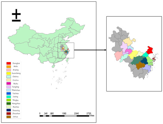
Figure 1.
The geographical location of the study area.
The data sources of this paper are the Statistical Yearbook of local statistics websites. The data of Shanghai, Zhejiang and Anhui are from the official website of the Municipal Bureau of Statistics (http://tjj.sh.gov.cn/, http://tjj.zj.gov.cn/, http://tjj.ah.gov.cn/) (accessed on 15 July 2022). Since the water consumption in each city in Jiangsu Province cannot be found in the Statistical Yearbook of Jiangsu Provincial Bureau of Statistics, Jiangsu Province is not included in the study area of this paper. Therefore, 17 cities are selected as the research areas of this paper.
3. Methods
The grey correlation in this paper is applied to analyze the relationship between water consumption and influence factors. Then, the DGM(1,N) with deformable accumulation (DDGM(1,N) model) is established to study the change trend of water consumption. Finally, the validity of the model is proven via model comparative analysis.
3.1. Grey Correlation Analysis
The changing trend of water consumption is affected by many factors. Grey correlation analysis is used to explore the correlation between research objects and influencing factors, and the calculation process is shown as follows.
(1) Set as the system characteristic behavior sequence, and as the sequence of relevant factors. Calculate the mean terms of each sequence using .
(2) Calculate the grey relational coefficients using Equation (1). For ,
(3) Calculate the grey relational degree using Equation (2).
3.2. The DDGM(1,N) Model
In this paper, the DGM(1,N) with deformable accumulation (DDGM(1,N) model) is used to predict the water consumption (billion cubic meters) of 17 cities selected in the Yangtze River Delta Economic Zone. The process is introduced as follows.
(1) Assume that the system principal variable data sequence is Equation (3).
The sequences of relevant factors are Equation (4).
is a sequence of cumulative generation operations of . Consider that the definition of the deformable derivative (Wu and Zhao, 2019) -order accumulation sequence is Equation (5).
The cumulative generation of the model is calculated using Equation (6).
The particle swarm optimization algorithm is used to find the optimal order () in MATLAB (R2016b). is the deformable accumulation parameter; it can adjust the weight of old and new data during sequence generation.
(2) The grey model DDGM(1,N) of the -order is Equation (7).
is the grey function system parameter of the model; is the principal variable parameter. are grey action system parameters of different independent variables in the model.
Then, the least squares method is used to solve the parameters in the model (Equation (8)). Therefore, the parameters and can be obtained by using Equations (9) and (10).
where
is recursive function of the DDGM(1,N) model. Then, the simulated value of can be obtained by using Equation (11).
According to Equation (12), we can see that the simulation value of is (see Equation (13)).
(4) The fitting error and prediction error are solved by calculating the mean absolute percentage error value (MAPE) according to Equation (14).
3.3. Properties of the Cumulative Generating Operator
Property 1.
When , the accumulation sequence is a monotonically increasing sequence. When , the accumulation sequence is a monotonically decreasing sequence. Otherwise, the accumulation sequence is not monotonic.
Proof.
Knowing that
Then,
Therefore, when , the accumulation sequence is a monotonically increasing sequence; when , the accumulation sequence is a monotonically decreasing sequence. Otherwise, the accumulation sequence is not monotonic.
The proof of Property 1 is completed. □
Property 2.
The larger the parameter , the larger the value obtained by accumulating the sequence.
Proof.
By assuming that we can obtain the following formulas.
Therefore, is true. This shows that the larger the parameter , the larger the value obtained by accumulating the sequence.
The proof of Property 2 is completed. □
3.4. Analysis and Discussion of Model Stability
Lemma 1.
Let ; the vector norm and matrix norm are compatible. If a matrix norm has , then the solutions of the inhomogeneous linear equations and satisfy
where
It can be known from Lemma 1 that matrix and matrix are original matrices, and matrix and matrix are perturbation matrices, which are perturbations of the solution. According to the matrix perturbation analysis, the perturbation bound of the solution can be obtained.
Theorem 1.
Assume that the solution of the DDGM(1,N) model is . If only is perturbed by , then the perturbation bound of the solution in this case is
Proof.
If only is perturbed by , it is equivalent to when .
where
It is obvious that we can obtain the value of .
In the same way,
We can also obtain the value of .
Therefore, and can be obtained.
According to Lemma 1, they can be obtained as follows:
Then, the perturbation bound of the solution can be obtained.
Theorem 2.
If only is perturbed by , then the perturbation bound of the solution in this case is
Proof.
If only is perturbed by , it is equivalent to when , where
The value of can be obtained.
In the same way,
The value of can be obtained.
Therefore, and can be obtained.
According to Lemma 1, they can be obtained as follows:
Then, the perturbation bound of the solution can be obtained.
Theorem 3.
If only is perturbed by , then the perturbation bound of the solution in this case is
Proof.
If only is perturbed by , it is equivalent to when , where
The value of can be obtained.
In the same way,
The value of can be obtained.
Therefore, and can be obtained.
According to Lemma 1, they can be obtained as follows:
Then, the perturbation bound of the solution can be obtained.
According to the analysis and proof presented above:
The disturbance bound of the model is correlated with the size of the sample . In the case of equivalent disturbance, the larger the number of samples, the larger the disturbance bound of the model. This indicates that as the number of samples increases, the disturbance bound of the model increases and stability becomes worse, which means that the grey model is suitable for the modeling of the “less data” problem.
When the sample size is unchanged, the particle swarm optimization algorithm can be used to adjust the parameter , so that the disturbance bound of the solution satisfies . That means is more sensitive to the solution than . It also indicates that new information is given more weight than old information. Therefore, the DDGM(1,N) model conforms to the new information priority principle.
3.5. The Case Study
This paper takes the relationship between water consumption and different factors in Jinhua City as an example. The original data of Jinhua presented in Table 1 are from 2010 to 2017. The relationship between population and water consumption is analyzed according to the results, as well as the industrial added value and water consumption. Following the method described in Section 3.1 above, we can obtain the results that . The results show that the population has the largest impact on the water consumption, followed by the added value of the primary industry and the secondary industry, and finally, the added value of the tertiary industry has the least impact on the water consumption.

Table 1.
Data on water consumption and related factors in Jinhua City from 2010 to 2017.
DDGM(1,N) model is constructed according to the original data in Table 1, and the calculation process is shown as follows.
(1) The water consumption sequence of Jinhua City from 2010 to 2017 is
The population of Jinhua City from 2010 to 2017 is
Then, the optimal order is obtained through the particle swarm optimization (PSO) algorithm in MATLAB (R2016b). The -order cumulative sequences are as follows:
(2)
According to Equations (9) and (10), the parameters and can be obtained.
(3) The simulated value of is obtained using Equation (11) as follows:
Finally, the fitting and prediction results can be obtained, and the validity can be tested using MAPE with fitting MAPE = 0.9022% and prediction MAPE = 1.36%, respectively.
The fitting and prediction results of DDGM(1,2), GM(1,1) and GM(1,2) are shown in Table 2. Compared with the two classical grey models, the fitting MAPE and prediction MAPE of DDGM(1,2) model are both the smallest. There is no significant difference between the fitting MAPE of DDGM(1,2) and GM(1,1), but the prediction MAPE of DDGM(1,2) is smaller than that of GM(1,1). As for GM(1,2), both the fitting MAPE and the prediction MAPE of DDGM(1,2) are much smaller than GM(1,2). Therefore, DDGM(1,2) model has better fitting and prediction performance, indicating that this model is more effective in predicting water consumption.
Table 2.
Comparison results between three models based on the population factor (units: billion cubic meters).
Similarly, the DDGM(1,2) model is constructed according to the water consumption and the added value of the tertiary industry shown in Table 1. The fitting and prediction results of the three models are shown in Table 3. It can be found that the fitting MAPE and prediction MAPE of the DDGM(1,2) model are smaller than those of GM(1,1) and GM(1,2). This further illustrates the effectiveness of the DDGM(1,2) model to predict water consumption.
Table 3.
Comparison results between three models based on the tertiary industry factor (units: billion cubic meters).
4. Forecasting Results and Discussion
In order to accurately predict the water consumption, we should consider the impact of three major industries and the population. However, the future changes of these variables are unknown. Therefore, this paper makes a hypothesis on the growth rate based on the government work report and urban development planning from recent years. Combined with different influencing factors, the DDGM(1,N) model was established to predict the urban water consumption. The calculation steps are the same as those in Section 3.2 in this paper. In this section, we predict the water consumption in the years of 2020–2025 using data from 2010 to 2019 for cities within Zhejiang Province and Shanghai. Due to the incompleteness of the data obtained in Anhui Province, the original data we had are from 2013 to 2019, so the forecasted range of water consumption in Anhui Province covers the years of 2020–2023.
4.1. Discussion on the Forecasting Results Combined with Population
The forecasting results for water consumption in the cities of Zhejiang Province are shown in Table 4 and Figure 2. As shown in Figure 2, the water consumption in Zhoushan will have an upward trend. However, the change in water consumption in Zhoushan is not significant compared with other cities. In the other seven cities, the water consumption shows a descending trend with the rise in population. In terms of numerical analysis, Hangzhou and Ningbo have a comparatively large population, so water consumption will also be at a high level. Water consumption in Huzhou, Jiaxing, Shaoxing, Jinhua and Taizhou will be at a moderate level. Due to the continuous increase in population and the increase in per capita income, personal and family consumption continue to increase, which has resulted in an increasing discharge of urban domestic sewage. Therefore, the government should adopt a series of control measures such as a tiered pricing mechanism for the management of water prices.
Table 4.
Forecasting results at different growth rates of population in Zhejiang (units: billion cubic meters).
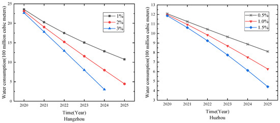
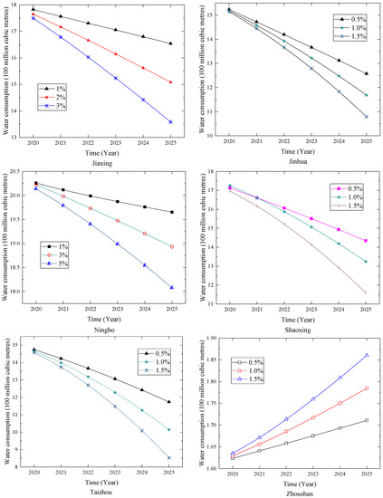
Figure 2.
Forecasting results for Zhejiang Province.
At present, many cities in the Yangtze River Delta have become water-scarce cities. The conservation and protection of water resources has become an urgent matter. The government should aim to improve water quality and protect the water system by establishing a water pollution prevention mechanism. It is strictly forbidden to develop high-risk and high-polluting industries at the source of rivers and upstream. At the same time, the population of these cities should be taken seriously. The government should also actively promote water conservation knowledge and carry out thematic activities related to the protection of resources so they can finally achieve the goal of improving people’s water conservation awareness.
Table 5 and Figure 3 show the prediction results for Shanghai at different growth rates of population. With the rise in the population growth rate, the water consumption in Shanghai will decline. During the process of rapid industrialization and urbanization, the influence of environmental factors on regional economic development is increasingly apparent. With the continuous emission and accumulation of pollutants from production activities and people’s daily lives, Shanghai is facing the pressure of regional environmental quality. At the same time, Shanghai as a densely populated city, and the problem of population control also brings challenges to the government’s management of water resources. Taihu Lake, the lower reaches of the Yangtze River, Qiantang River and other water resources are polluted in different degrees, while Taihu Lake is the most serious. At present, only 1% of the surface water in Shanghai meets the national standard of drinking water sources. Water pollution makes this area, which has abundant water resources, gradually become a water shortage region.
Table 5.
Forecasting results at different growth rates of population in Shanghai (units: billion cubic meters).
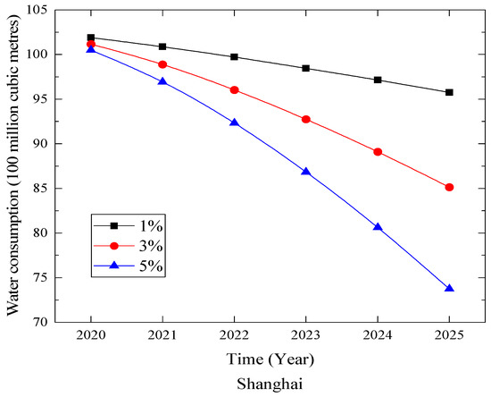
Figure 3.
Forecasting results for Shanghai.
The forecasting results for Anhui Province under different population growth rates are shown in Table 6 and Figure 4. The water consumption in Anqing, Chuzhou, Hefei and Maanshan in Anhui Province decrease with the increase in population. This shows that under the correct guidance of these city governments and with the reasonable and effective control of water resources, the water conservation awareness of residents and the protection of resources improve. With the change in the population growth rate, the tendency of water consumption in Xuancheng inclines to present a consistently downward trend. This shows that the effect of demographic factors on the changes in water consumption in Xuancheng is not obvious, and it can be analyzed from other aspects. When the population shows a negative growth, the water consumption in Tongling declines. When the population shows a positive growth trend, the water consumption in Tongling begins to show an upward trend. This indicates that the population factor has an impact on the change in water consumption. So, we should pay attention to the population management of the city to achieve better results in the management of water resources.
Table 6.
Forecasting results at different growth rates of population in Anhui (units: billion cubic meters).
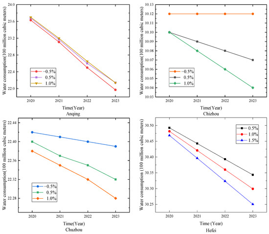
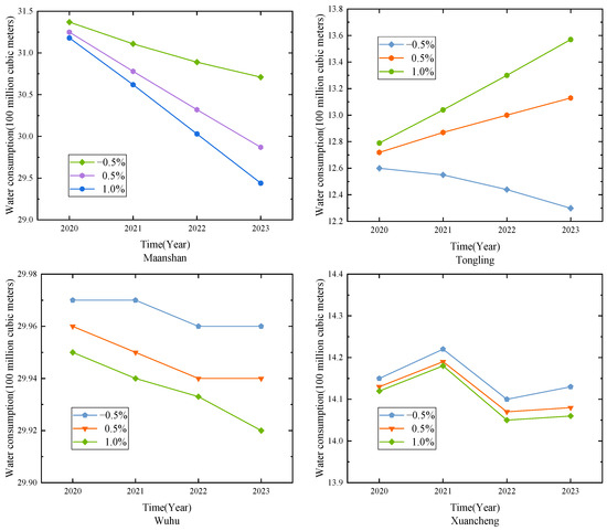
Figure 4.
Forecasting results for Anhui Province.
4.2. Discussion on the Forecasting Results Combined with the Primary Industry
The forecasting results for the cities in Zhejiang Province under different growth rates of the added value of the primary industry are shown in Table 7 and Figure 5. The figure shows that the prediction results for six cities will descend with the rise in the added value of the primary industry. On the one hand, people’s water conservation awareness in these areas was improved, and the water-saving technology industry was improved. On the other hand, due to the growth of the primary industry, the government has strengthened the control and protection of water resources. The trend of water consumption in Jiaxing and Zhoushan is different from that in other cities. The faster the primary industry develops, the greater the annual water consumption. However, compared with other cities, the population base of Zhoushan is relatively small, and the expansion of the primary industry is relatively backward. Therefore, the change in the water consumption is not obvious.
Table 7.
Forecasting results at different growth rates of the primary industry in Zhejiang (units: billion cubic meters).
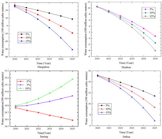
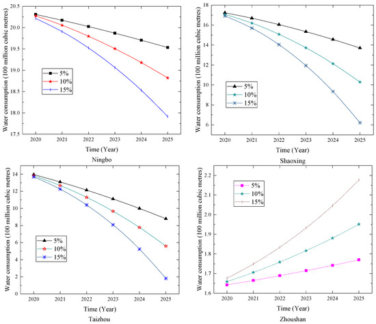
Figure 5.
Forecasting results for Zhejiang Province.
Table 8 and Figure 6 show the prediction results for Shanghai. With the accelerated growth in the primary industry, the water consumption in the city has shown a downward trend. This shows that the government’s management is effective. The agriculture and animal husbandry industries that emit large amounts of pollutants are carefully governed to reduce the pressure on the environment. Shanghai is a leader in the economic integration of the Yangtze River Delta and, accompanied with the economic transformation and construction of an international metropolis, Shanghai has a huge spillover effect on the development of the surrounding cities. In terms of water management and control, Shanghai should continue to maintain its current momentum. Agriculture that pollutes the environment should continue to be paid attention to and given management measures. Furthermore, Shanghai should promote the construction of a water-saving society in an all-around and in-depth manner.
Table 8.
Forecasting results at different growth rates of the primary industry in Shanghai (units: billion cubic meters).
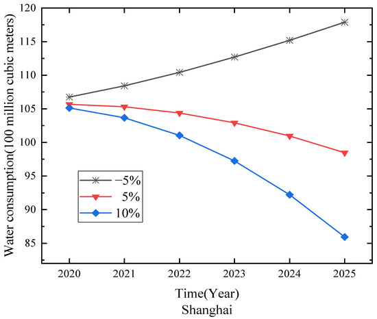
Figure 6.
Forecasting results for Shanghai.
The prediction results for water consumption in the cities of Anhui Province are shown in Table 9 and Figure 7. When the primary industry increases, the annual water consumption in Chuzhou, Hefei and Ma’anshan will show a downward trend. The greater the growth rate of the primary industry is, the faster the reduction in water consumption will be. The change trend of water consumption in Tongling and Wuhu is very similar. A faster growth rate of water consumption will emerge when the growth rate of the primary industry is higher. Water consumption in Chizhou shows an upward trend when the assumed growth rate increases. This shows that there is an important relationship between Chizhou’s primary industry and water consumption. When the growth rate changes, Xuancheng will always show a downward trend. Anqing’s annual water consumption has shown a downward trend. Therefore, the cities should continue to strengthen the evolution and upgrading of technology on the preservation of the environment, which ultimately helps to achieve the aim of improving efficiency.
Table 9.
Forecasting results at different growth rates of the primary industry in Anhui (units: billion cubic meters).
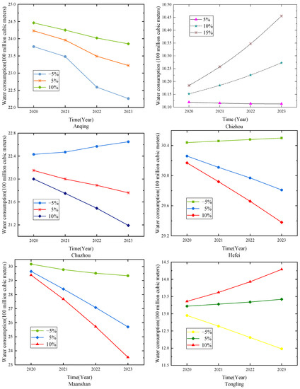
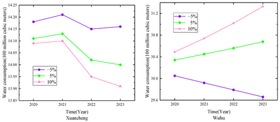
Figure 7.
Forecasting results for Anhui Province.
4.3. Discussion on the Forecasting Results Combined with the Secondary Industry
The forecasting results for the cities in Zhejiang Province under different change rates of the added value of the secondary industry are shown in Table 10 and Figure 8. With the rise in the added value of the secondary industry, the annual water consumption in cities except for Zhoushan all show a downward trend. This shows that under the guidance of the government’s intervention in the secondary industry, good water-saving results were achieved in water resources management. For example, Hangzhou issued a “water limit order” to 212 companies that use more than 10,000 tons of water per month. Shaoxing launched a water-saving campaign for the eight major water-consuming industries, including thermal power, chemical industry, and papermaking; other cities adopted various water-saving measures. It is recommended that the water-saving management departments in various cities should strengthen their communication and exchanges of experience in building a water-saving society. Therefore, we should jointly seek the key points of conservation in cities with “water-quality water shortage”.
Table 10.
Forecasting results at different growth rates of the secondary industry in Zhejiang (units: billion cubic meters).
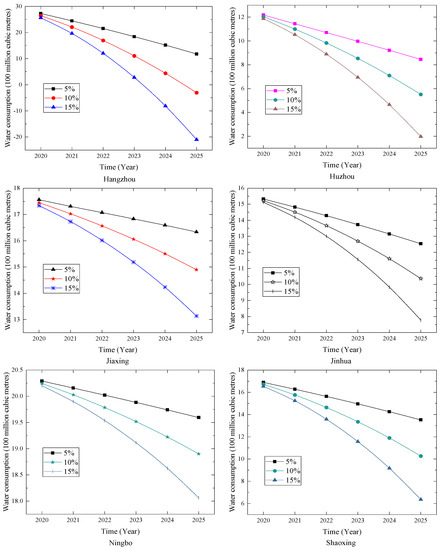
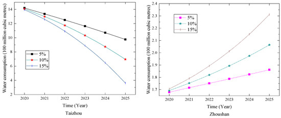
Figure 8.
Forecasting results for Zhejiang Province.
The water consumption in Zhoushan has shown an upward trend, but the base and change in water consumption are very small. This is because compared with other cities, Zhoushan’s industry and construction are not well developed, and the speed of economic growth is comparatively slow, which is limited by the geographical conditions of Zhoushan. Zhoushan is composed of many islands, so it faces many problems in terms of transportation.
Table 11 and Figure 9 show the forecasting results for Shanghai under different growth rates of the secondary industry added value. The faster the secondary industry grows, the faster the water consumption will decrease. This shows that the efforts made in Shanghai to promote the construction of a water-saving society have achieved excellent results. The government implements and improves a strict water resources management system to fundamentally facilitate water conservation. The water resources management department conducts regular inspections of water-using enterprises. Through the formulation and implementation of water-saving measures, the water-saving potential of enterprises and industrial water-saving technologies can be tapped. Meanwhile, through the innovation and application of technology, the recycling utilization rate of industrial water was improved.
Table 11.
Forecasting results at different growth rates of the secondary industry in Shanghai (units: billion cubic meters).
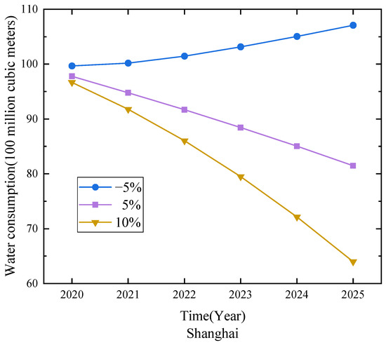
Figure 9.
Forecasting results for water consumption in Shanghai.
The forecasting results for the cities in Anhui Province under different growth rates of the secondary industry added value are shown in Table 12 and Figure 10. The results show that the water consumption in Anqing, Ma’anshan and Xuancheng decrease with the rise in the added value of the secondary industry. This is because these cities have high industrial water utilization and advanced industrial water-saving technologies. The change trends of water consumption in Tongling and Wuhu are very similar. Water consumption will decline with the development of the secondary industry in these cities. Water consumption in Chizhou will rise with the increase in the growth rate. This shows that with the expansion of the city’s size, the scale and number of industries have increased, which further led to an increase in industrial water consumption, which, in turn, triggered the rise in Chizhou’s water consumption. With the development of the secondary industry added value, the water consumption in Hefei will show a downward trend because Hefei increased the utilization rate of industrial water by improving water-saving technologies. Therefore, the local government should strengthen the management and control of industrial water and increase the utilization rate of industrial water.
Table 12.
Forecasting results at different growth rates of the secondary industry in Anhui (units: billion cubic meters).
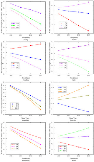
Figure 10.
Forecasting results for water consumption in Anhui Province.
4.4. Discussion on the Forecasting Results Combined with the Tertiary Industry
The forecasting results for the cities in Zhejiang Province are shown in Table 13 and Figure 11. The results show that except for Zhoushan, the water consumption in the other seven cities present a downward trend because these cities pay more attention to water management, e.g., in the technical transformation and upgrading of water-using equipment for industries with high water consumption such as accommodation, catering and real estate. At the same time, the adjustment of water prices can also help to achieve the goal of improving water efficiency. With the development of the tertiary industry, Zhoushan’s annual water consumption has shown a gentle upward trend. Compared with other cities, Zhoushan’s economic development is lagging, and the growth of the tertiary industry is also at a low level. Therefore, the water consumption in Zhoushan is kept at a low level.
Table 13.
Forecasting results at different growth rates of the tertiary industry in Zhejiang (units: billion cubic meters).
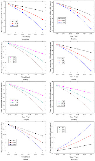
Figure 11.
Forecasting results for Zhejiang Province.
Table 14 and Figure 12 show the forecasting results for Shanghai under different growth rates of the tertiary industry. It is shown that a downtrend will present in the next few years. This is because Shanghai has strengthened their management of water resources by launching a number of water-saving campaigns to raise people’s awareness of the importance of saving water. Regarding the remediation of industries with a high water consumption, the water resources management department has carried out measures by adjusting water prices, updating water-saving equipment and upgrading water-saving technologies.
Table 14.
Forecasting results at different growth rates of the tertiary industry in Shanghai (units: billion cubic meters).
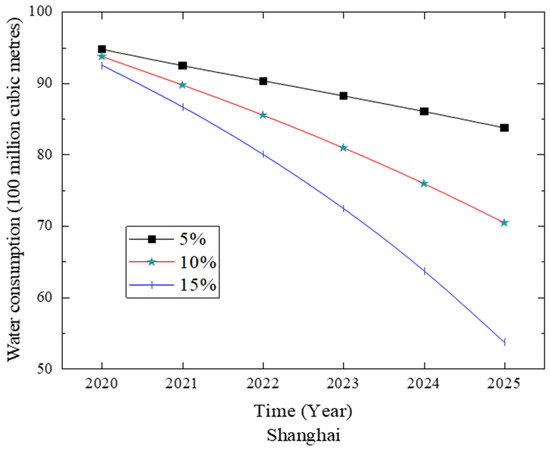
Figure 12.
Forecasting results for Shanghai.
The forecasting results for water consumption in the cities of Anhui Province are shown in Table 15 and Figure 13. We can find that the trends of water consumption in Chizhou, Chuzhou, Hefei and Tongling are very similar. The rise in water consumption accelerates as the growth rate of the tertiary industry increases. It is suggested that these cities should control the growth speed of the tertiary industry so as to avoid excessively fast economic growth from putting a huge pressure on the resources and environment. Traditional high-polluting industries such as the printing and dyeing, papermaking and chemical industries still account for a relatively high share, while the proportion of high-tech industries and service industries is still relatively small in these cities. The annual water consumption in Anqing, Ma’anshan, Wuhu and Xuancheng decrease. The government departments of these cities are actively carrying out water-saving-related activities. The water efficiency has been improved by raising water prices and improving reclaimed water utilization technology. Through these methods, the coordinated development between water use and economic development can be achieved.
Table 15.
Forecasting results at different growth rates of the tertiary industry in Anhui (units: billion cubic meters).
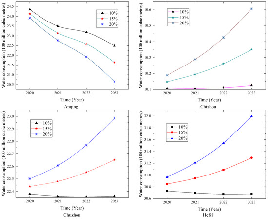
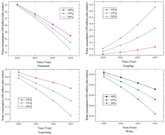
Figure 13.
Forecasting results for Anhui Province.
5. Conclusions
This article firstly uses the grey relational analysis to study the related factors affecting water consumption. Then, through the model comparisons, we found that the DDGM(1,N) model has a better fitting and prediction effect. Finally, the DDGM (1,N) model was used to predict the water consumption in 17 cities selected in the Yangtze River Delta region by considering different influencing factors. The results show that as the growth rate of the population increases, the water consumption in 15 cities show a downward trend, and 2 cities show an upward trend. With the increase in the growth rate of the primary industry, the water consumption in 12 cities show a downward trend, and 5 cities show an upward trend. With the rise in the growth rate of the secondary industry, the water consumption in 14 cities show a downward trend, and 3 cities show an upward trend. With the rise in the growth rate of the tertiary industry, the water consumption in 12 cities show a downward trend, and 5 cities show an upward trend. In general, the water consumption in most cities will continue to show a downward trend in the future.
According to the prediction results obtained in this paper, we have some policy recommendations as follows. First of all, urban populations should be controlled. We should avoid a situation where the population density is concentrated, which will cause great pressure on the water consumption. Secondly, for cities where water consumption has increased with the development of the primary industry, the water resource utilization efficiency of agriculture and animal husbandry should be improved. Moreover, for cities where the water consumption increases with the development of the secondary industry, it is suggested that they adjust the internal structure of the secondary industry to reduce the proportion of high water-consuming industries, and meanwhile, strengthen the supervision of industrial water efficiency. It is possible to raise the utilization rate by adjusting the water prices and upgrading the water-saving technologies of water-using equipment. Finally, for cities whose water consumption has increased with the development of the tertiary industry, the service industries of these cities should shift to the direction of eco-environmental protection. We should focus on the accommodation and catering industry, carry out technical transformation of its water equipment and eliminate outdated high water-consuming equipment simultaneously. Through the government’s management and policy guidance, the goal of improving the utilization effect of water resources is realized.
Author Contributions
Conceptualization, Z.Q. and W.Y.; methodology, Z.Q.; software, Z.Q.; validation, Z.Q., W.Y.; formal analysis, Z.Q.; investigation, Z.Q.; resources, Z.Q.; data curation, Z.Q.; writing—original draft preparation, Z.Q.; writing—review and editing, W.Y.; visualization, Z.Q.; supervision, W.Y.; project administration, W.Y.; funding acquisition, W.Y. All authors have read and agreed to the published version of the manuscript.
Funding
This research was funded by the National Natural Science Foundation of China (NSFC) under grant No. 71971131; the MOE (Ministry of Education in China) Youth Project of Humanities and Social Sciences Fund under grant number 17YJC630121; the Research Project Supported by Shanxi Scholarship Council of China under grant No. 2022–027. And The APC was funded by Wei Yang.
Data Availability Statement
The data sources are the Statistical Yearbook of local statistics web-sites. The data of Shanghai, Zhejiang and Anhui are from the official website of the Municipal Bureau of Statistics (http://tjj.sh.gov.cn/, http://tjj.zj.gov.cn/, http://tjj.ah.gov.cn/) (accessed on 15 July 2022).
Acknowledgments
The relevant research is supported by the National Natural Science Foundation of China (NSFC) under grant No. 71971131; the MOE (Ministry of Education in China) Youth Project of Humanities and Social Sciences Fund under grant number 17YJC630121; the Research Project Supported by Shanxi Scholarship Council of China under grant No. 2022−027.
Conflicts of Interest
The authors declare no conflict of interest.
References
- Fan, J.-L.; Wang, J.-D.; Zhang, X.; Kong, L.-S.; Song, Q.-Y. Exploring the changes and driving forces of water footprints in China from 2002 to 2012: A perspective of final demand. Sci. Total Environ. 2019, 650, 1101–1111. [Google Scholar] [CrossRef] [PubMed]
- Li, S.; Han, W. Performance evaluation for urban water supply services in China. Water Supply 2020, 20, 3511–3516. [Google Scholar] [CrossRef]
- Bata, M.H.; Carriveau, R.; Ting, D.S.-K. Short-Term Water Demand Forecasting Using Nonlinear Autoregressive Artificial Neural Networks. J. Water Resour. Plan. Manag. 2020, 146, 04020008. [Google Scholar] [CrossRef]
- Mensik, P.; Marton, D. Hybrid Optimization Method for Strategic Control of Water Withdrawal from Water Reservoir with Using Support Vector Machines. Procedia Eng. 2017, 186, 491–498. [Google Scholar] [CrossRef]
- Tarebari, H.; Javid, A.H.; Mirbagheri, S.A.; Fahmi, H. Multi-Objective Surface Water Resource Management Considering Conflict Resolution and Utility Function Optimization. Water Resour. Manag. 2018, 32, 4487–4509. [Google Scholar] [CrossRef]
- Vonk, E.; Cirkel, D.G.; Blokker, M. Estimating Peak Daily Water Demand under Different Climate Change and Vacation Scenarios. Water 2019, 11, 1874. [Google Scholar] [CrossRef]
- Pei, X.; Sun, Y.; Ren, Y. Demand estimation of water resources via bat algorithm. Int. J. Wirel. Mob. Comput. 2020, 18, 16–21. [Google Scholar] [CrossRef]
- Shao, Z.; Wu, F.; Li, F.; Zhao, Y.; Xu, X. System Dynamics Model for Evaluating Socio-Economic Impacts of Different Water Diversion Quantity from Transboundary River Basins—A Case Study of Xinjiang. Int. J. Environ. Res. Public Health 2020, 17, 9091. [Google Scholar] [CrossRef]
- Mu, L.; Zheng, F.; Tao, R.; Zhang, Q.; Zoran Kapelan, Z. Hourly and Daily Urban Water Demand Predictions Using a Long Short-Term Memory Based Model. J. Water Resour. Plan. Manag. 2020, 146, 05020017. [Google Scholar] [CrossRef]
- Araujo, W.C.; Esquerre, K.P.O.; Sahin, O.; Silva, B.B.S. Scarcity Pricing for Water Demand Management: A Case Study in Campina Grande-Brazil. J. Environ. Account. Manag. 2021, 9, 75–91. [Google Scholar] [CrossRef]
- Anderson, B.; Manouseli, D.; Nagarajan, M. Estimating scenarios for domestic water demand under drought conditions in England and Wales. Water Sci. Technol. Water Supply 2018, 18, 2100–2107. [Google Scholar] [CrossRef]
- Gibson, J.; Karney, B.; Guo, Y. Effects of Demand, Mixing Fraction, and Rate Coefficient Uncertainty on Water Quality Models. J. Water Resour. Plan. Manag. 2020, 146, 06020004. [Google Scholar] [CrossRef]
- Massoud, B.; Reza, K. Evaluating the resilience of water resources management scenarios using the evidential reasoning approach: The Zarrinehrud river basin experience. J. Environ. Manag. 2021, 284, 112025. [Google Scholar] [CrossRef]
- Maria, X.; Chris, H.; Jan, H.; Zoran, K. Short-Term Forecasting of Household Water Demand in the UK Using an Interpretable Machine-Learning Approach. J. Water Resour. Plan. Manag. 2021, 147, 04021004. [Google Scholar] [CrossRef]
- Berthe, Y.A.; Jules, M.O.M.; Sampah, G.E.; Alioune, K.; Albert, G.B.T. Using “Water Evaluation and Planning” (WEAP) Model to Simulate Water Demand in Lobo Watershed (Central-Western Cote d’Ivoire). J. Water Resour. Prot. 2021, 13, 216–235. [Google Scholar] [CrossRef]
- Tu, L.; Chen, Y. An unequal adjacent grey forecasting air pollution urban model. Appl. Math. Model. 2021, 99, 260–275. [Google Scholar] [CrossRef]
- Rees, P.L.S. Advancing Agricultural Water Security and Resilience Under Nonstationarity and Uncertainty: Evolving Roles of Blue, Green, and Grey Water. J. Contemp. Water Res. Educ. 2018, 165, 1–3. [Google Scholar] [CrossRef]
- Kose, E.; Tasci, L. Geodetic deformation forecasting based on multi-variable grey prediction model and regression model. Grey Syst. Theory Appl. 2019, 9, 464–471. [Google Scholar] [CrossRef]
- Jamshidi, S. An approach to develop grey water footprint accounting. Ecol. Indic. 2019, 106, 105477. [Google Scholar] [CrossRef]
- Ma, D.; Duan, H.; Li, W.; Zhang, J.; Liu, W.; Zhou, Z. Prediction of water inflow from fault by particle swarm optimization-based modified grey models. Environ. Sci. Pollut. Res. Int. 2020, 27, 42051–42063. [Google Scholar] [CrossRef]
- Li, B.; Wu, Q.; Zhang, W.; Liu, Z. Water resources security evaluation model based on grey relational analysis and analytic network process: A case study of Guizhou Province. J. Water Process Eng. 2020, 37, 101429. [Google Scholar] [CrossRef]
- Zhang, K.; Zhong, Q.; Qu, P.; Yin, Y.; Zuo, Y. Rural water environment quality grey prediction model based on network search information. Chin. Manag. Sci. 2020, 28, 222–230. [Google Scholar]
- Liao, X.; Chai, L.; Liang, Y. Income impacts on household consumption’s grey water footprint in China. Sci. Total Environ. 2021, 755, 142584. [Google Scholar] [CrossRef] [PubMed]
- Ju, Q.; Hu, Y. Source identification of mine water inrush based on principal component analysis and grey situation decision. Environ. Earth Sci. 2021, 80, 157. [Google Scholar] [CrossRef]
- Meng, X.; Wu, L. Prediction of per capita water consumption for 31 regions in China. Environ. Sci. Pollut. Res. 2021, 28, 29253–29264. [Google Scholar] [CrossRef]
- Deng, J. Control problems of grey systems. Syst. Control Lett. 1982, 1, 288–294. [Google Scholar] [CrossRef]
- Guo, J.; Tu, L.; Qiao, Z.; Wu, L. Forecasting the air quality in 18 cities of Henan Province by the compound accumulative grey model. J. Clean. Prod. 2021, 310, 127582. [Google Scholar] [CrossRef]
- Wang, Z.; Dang, Y.; Liu, S. Optimization of Background Value in GM(1,1) Model. Syst. Eng. Theory Pract. Online 2008, 28, 61–67. [Google Scholar] [CrossRef]
- Ma, X.; Liu, Z. Application of a novel time-delayed polynomial grey model to predict the natural gas consumption in China. J. Comput. Appl. Math. 2017, 324, 17–24. [Google Scholar] [CrossRef]
- Zeng, B.; Duan, H.; Bai, Y.; Meng, W. Forecasting the output of shale gas in China using an unbiased grey model and weakening buffer operator. Energy 2018, 151, 238–249. [Google Scholar] [CrossRef]
- Chen, Y.; Yang, Y. A Multivariate Statistical Model of Water Leakage in Urban Water Supply Networks Based on Random Matrix Theory. Math. Probl. Eng. 2022, 2022, 2314972. [Google Scholar] [CrossRef]
- Li, M.; Cheng, Z.; Lin, W.; Wei, Y.; Wang, S. What can be learned from the historical trend of crude oil prices? An ensemble approach for crude oil price forecasting. Energy Econ. 2023, 123, 106736. [Google Scholar] [CrossRef]
- Liu, L.; Chen, Y.; Wu, L. The damping accumulated grey model and its application. Commun. Nonlinear Sci. Numer. Simul. 2021, 95, 105665. [Google Scholar] [CrossRef]
- Duan, H.; Pang, X. A novel grey prediction model with system structure based on energy background: A case study of Chinese electricity. J. Clean. Prod. 2023, 390, 136099. [Google Scholar] [CrossRef]
- Wu, L.; Zhao, H. Discrete grey model with the weighted accumulation. Soft Comput. 2019, 23, 12873–12881. [Google Scholar] [CrossRef]
- Li, Y.; Li, J. Study on unbiased interval grey number prediction model with new information priority. Grey Syst. Theory Appl. 2019, 10, 1–11. [Google Scholar] [CrossRef]
- Huynh, N.T.; Nguyen, T.V.T.; Tam, N.T.; Nguyen, Q.M. Optimizing Magnification Ratio for the Flexible Hinge Displacement Amplifier Mechanism Design. In Proceedings of the 2nd Annual International Conference on Material, Machines and Methods for Sustainable Development (MMMS2020), MMMS 2020, Lecture Notes in Mechanical Engineering, Nha Trang, Vietnam, 12–15 November 2020; Long, B.T., Kim, Y.H., Ishizaki, K., Toan, N.D., Parinov, I.A., Vu, N.P., Eds.; Springer: Cham, Switzerland, 2021; pp. 769–778. [Google Scholar] [CrossRef]
Disclaimer/Publisher’s Note: The statements, opinions and data contained in all publications are solely those of the individual author(s) and contributor(s) and not of MDPI and/or the editor(s). MDPI and/or the editor(s) disclaim responsibility for any injury to people or property resulting from any ideas, methods, instructions or products referred to in the content. |
© 2023 by the authors. Licensee MDPI, Basel, Switzerland. This article is an open access article distributed under the terms and conditions of the Creative Commons Attribution (CC BY) license (https://creativecommons.org/licenses/by/4.0/).