Article

Federated Learning Incentive Mechanism Design via Shapley Value and Pareto Optimality

1
School of Mathematics and Statistics, Guizhou University, Guiyang 550025, China
2
State Key Laboratory of Public Big Data, College of Computer Science and Technology, Guizhou University, Guiyang 550025, China
3
Guizhou Big Data Academy, Guizhou University, Guiyang 550025, China
4
Key Laboratory of Advanced Manufacturing Technology, Ministry of Education, Guizhou University, Guiyang 550025, China
5
College of Big Data and Information Engineering, Guizhou University, Guiyang 550025, China
6
School of Information, Guizhou University of Finance and Economics, Guiyang 550025, China
*
Author to whom correspondence should be addressed.
Axioms 2023, 12(7), 636; https://doi.org/10.3390/axioms12070636
Submission received: 7 May 2023 / Revised: 16 June 2023 / Accepted: 25 June 2023 / Published: 27 June 2023
(This article belongs to the Special Issue Advances in Logic and Game Theory)

Abstract

:
Federated learning (FL) is a distributed machine learning framework that can effectively help multiple players to use data to train federated models while complying with their privacy, data security, and government regulations. Due to federated model training, an accurate model should be trained, and all federated players should actively participate. Therefore, it is crucial to design an incentive mechanism; however, there is a conflict between fairness and Pareto efficiency in the incentive mechanism. In this paper, we propose an incentive mechanism via the combination of the Shapley value and Pareto efficiency optimization, in which a third party is introduced to supervise the federated payoff allocation. If the payoff can reach Pareto optimality, the federated payoff is allocated by the Shapley value method; otherwise, the relevant federated players are punished. Numerical and simulation experiments show that the mechanism can achieve fair payoff allocation and Pareto optimality payoff allocation. The Nash equilibrium of this mechanism is formed when Pareto optimality payoff allocation is achieved.
MSC:
91A12; 91A06; 58E17

1. Introduction

As artificial intelligence (AI) continues to develop at a rapid pace, massive and diverse data are rapidly being generated. Data from all walks of life have high utility value and privacy information. In particular, there are data islands and data privacy problems. To solve the problems of data islands and data privacy, McMahan et al. [1,2,3] proposed a distributed machine learning method called federated learning (FL) in 2016. FL is used to train the model at each node, and their own sensitive data are not leaked, which not only makes full use of the data to train models but also protects sensitive data privacy [4].
However, in the FL process, to make each data owner willing to contribute their data to train the model and improve the accuracy of the model, designing an incentive mechanism in the FL system is a valuable research topic. If there is a phenomenon of free riding among federated players, such as the lack of real-time training data, the accuracy of federated model training will be seriously affected. Therefore, establishing an attractive incentive mechanism is valuable research work in the FL system.
Nowadays, the FL incentive mechanism has attracted much attention from academics [5,6]. They have conducted a lot of research in [7,8,9], and although they considered fairness [10,11], they did not consider the Pareto optimality efficiency. We aim to establish an incentive model in a federated system to achieve fair payoff allocation and Pareto optimality. For this purpose, we propose a method via the Shapley value and Pareto optimality. Since the Shapley value is consistent with the principle of budget balance, however, according to Holmstrom’s team production theory [12], budget balance and Pareto optimality cannot be reached simultaneously. Therefore, although the Shapley value method can satisfy fair payoff allocation after the completion of FL, it cannot achieve the optimality incentive input of each federated player before FL, i.e., it cannot achieve Pareto efficiency optimization before FL. Therefore, we design this mechanism for the payoff allocation of FL to make the payoff allocation of FL fair and efficient. We introduce supervisor and set penalty conditions. If the federated payoffs reach Pareto efficiency optimality, the payoffs are allocated by Shapley’s value formula; otherwise, the relevant federated players are penalized. Finally, numerical experiments are performed to confirm our theoretical analysis. The main contributions of the paper can be summarized as follows:
(1)
Discussing the conditions satisfied by the fines paid to the regulator by the limited-liability federated agent if Pareto optimality is achieved;
(2)
Demonstrating that the federated players’ inputs constitute the mechanism’s Nash equilibrium when Pareto optimality is satisfied;
(3)
Numerical examples are performed to verify the rationality of designing the mechanism for the both equal and unequal statuses of the federated players.
The remaining work is organized as follows: The related work is introduced in Section 2. The preliminaries are introduced in Section 3. The FL incentive mechanism is established in Section 4. The rationality of this incentive mechanism is verified by numerical and simulation experiments in Section 5. The conclusion and future work are drawn in Section 6. The discussion is drawn in Section 7. The proof of the theorem is given in Appendix A.

2. Related Work

The main theoretical approaches currently used for the FL incentive mechanism include the Stackelberg game [13], contract theory [14], auction mechanism [15] and Shapley value [16]. In this paper, we review the research works related to the FL incentive mechanism design by the Shapley value. In [17], Song et al. proposed a new Shapley value based on the contribution metric to evaluate the contribution of each player who owns the data for the training of the FL model. In [18], the authors proposed a new expression for the Shapley value for FL, which can be computed without consuming additional communication costs, can play a role in the value of the FL data, and can have an incentive effect on the players. Wang et al. [19] used the Shapley value to fairly calculate each federated player’s contribution. To properly incentivize data owners to contribute their data to train the federated model, in [20], the authors proposed a blockchain-based peer-to-peer payment system for FL to achieve a feasible fair payoff allocation mechanism based on the Shapley value. In the literature [21], a fair incentive mechanism based on the Shapley value was proposed. This can motivate more players to be willing to share their data and receive a certain fee. In [22], the authors proposed the bootstrap truncated gradient Shapley approach for the fair valuation of the FL players’ contributions. This approach mainly reconstructs the FL model from gradient updates for Shapley value calculation. Nagalapattiet et al. [23] proposed a cooperative game, where players share gradients and compute players’ Shapley values to filter those with relevant data. To address the fact that there are still other inequities in calculating the FL Shapley value, Fan et al. [24] proposed a new complete federated Shapley value mechanism to improve the fairness of the federated Shapley value. In addition, to address the fact that the calculation of the Shapley value in FL requires a certain communication cost, in [25], the authors proposed a Shapley value based on a contribution evaluation metric called the vertical federated Shapley value (VerFedSV) and verified the fairness of VerFedSV through experiments. In [26], the authors considered several factors affecting FL and proposed an FL incentive mechanism according to the enhanced Shapley value method, and numerical experiments verified that the payoffs allocated among all participants can be fairer when using the enhanced Shapley value method.

3. Preliminaries

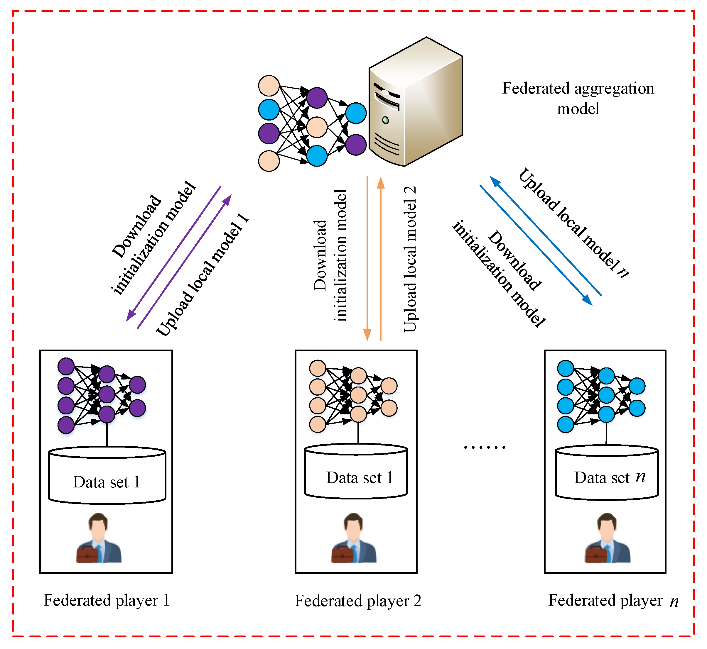
3.1. Federated Learning Framework

Federated learning (FL) is a distributed machine learning technique or machine learning framework. The goal of FL is to technically break down data silos and enable AI collaboration, where participants’ data do not leave the local area during the model training process, to achieve common modeling based on ensuring data privacy, and security and legal compliance [1].
Let N = { 1 , 2 , , n } be defined as n data players and participate in the training model M; their local dataset is D = { D 1 , D 2 , , D n } . M F E D denotes the shared model that FL requires players to train together, and M S U M denotes the traditional machine learning model, which puts all data together to train the model. V F E D and V S U M are the model accuracy of M F E D and M S U M , respectively, if there exists a positive number δ 0 which satisfies
| V F E D V S U M | < δ ,
we say that the FL algorithm has δ -accuracy loss [4].
The framework diagram of FL is shown in Figure 1, and the training steps in the FL model are as follows:
Step 1: Local federated players download the initialized global model from the aggregation server;
Step 2: Each federated player trains the local model with the initializing global model;
Step 3: After training the local model, the updated model and parameters are uploaded to the aggregation server;
Step 4: The aggregation server aggregates the models and parameters uploaded by each federated player for the next update round.
The commonly used aggregation method is the federated averaging (FedAvg) algorithm [27], Steps 2 and 3 are repeated until the local model converges.

3.2. Cooperative Games

Let G ( N , v ) be a defined cooperative game, satisfying the following conditions [28]:
v ( S 1 ) + v ( S 2 ) v ( S 1 S 2 ) ,
S 1 S 2 = , v ( ) = 0 .
where N is a finite set of players, S 1 , S 2 2 N , v : 2 N R is a game-characteristic function, and 2 N is the set of all the subsets of N. Let v ( S ) be the players’ payoff function, v ( N ) indicate the coalition payoff, and φ i ( v ) be the payoff of player i in v ( N ) , which satisfy two constraints:
v ( N ) = φ i ( v ) and v ( i ) φ i ( v ) , i N , i = 1 , 2 , , n ,
v ( S ) i S φ i ( v ) , S N , S .
Formulas (4) and (5) are called individual rationality and coalition rationality, respectively.

3.3. Shapley Value

The Shapley value was proposed in the cooperative game theory [28], which can effectively solve the problem of cooperative payoff allocation and is defined as
φ i ( v ) = i S , S N w ( | S | ) v ( S ) v ( S i ) ,
w ( | S | ) = ( n | S | ) ! ( | S | 1 ) ! n ! .
where S N , i S , i = 1 , 2 , , n , | S | is the number of players in subset S, w ( | S | ) is the weight coefficient, v ( S ) is the profit of subset | S | and satisfies the conditions (2) and (3), the expression v ( S ) v ( S i ) assesses the marginal contribution of i to the coalition S, and v ( S i ) indicates the payoff of the other players in the subset | S | other than i.

3.4. Pareto Optimality

Let π = π 1 , π 2 , , π n : x R n be the vector of the players’ payoff function, and x be a feasible action space for two actions x 1 and x 2 x [29]:
(1)
If i [ n ] : π i ( x 1 ) π i x 2 , then x 1 weakly dominates x 2 and is marked by x 1 x 2 ;
(2)
If x 1 x 2 and i [ n ] : π i ( x 1 ) > π i x 2 , then x 1 dominates x 2 and is marked by x 1 x 2 .
If no other action in x dominates it and the collection of the players’ action vectors of all Pareto optimality actions is the Pareto front, then an action is called the Pareto optimality [29]. In other words, an allocation is considered to be Pareto optimality if no alternative allocation could make someone better off without making someone else worse off [30].

3.5. Nash Equilibrium

We consider a game with n players, and the set of players is denoted as N = { 1 , 2 , , n } . The player i’s payoff function is π i ( x ) , where x = x 1 , x 2 , , x n T R n is the vector of the player’s actions, and x i R is the action of player i. If player j is not a neighbor of player i, then player i has no direct access to player j’s action.
Nash equilibrium is an action profile on which no player can gain more payoff by unilaterally changing its action, i.e., an action profile x * = x i * , x i * is the Nash equilibrium [31,32] if
π i x i * , x i * π i x i , x i * , i N
where x i = x 1 , x 2 , , x i 1 , x i + 1 , , x n T . Note that π i ( x ) and π x might alternatively be written as π i x i , x i and x i , x i , respectively, in this paper.

4. Federated Learning Incentive Mechanism

4.1. The FL Incentive Model

We make the following assumptions before setting up the FL incentive model:
(1)
All players can pay for FL, and in the payoff distribution process, they adopt the best payoff distribution scheme.
(2)
All players are satisfied with the final distribution of payoffs, as all players were willing to join the coalition.
(3)
All players are entirely trustworthy and have no cheating in the FL.
(4)
To ensure the smooth implementation of the strategy, the FL should adopt a multi-party agreement to accept the payoff distribution plan.
According to the idea of FL, we establish the FL incentive model in Figure 2, and the main steps of the FL incentive mechanism are as follows:
Step 1: Assume that there are n players for federated model training, and each player has its local dataset D i .
Step 2: Each player downloads the initialized model from the aggregation server, trains the model using its local dataset D i , and uploads the trained model m i to the federated aggregation server.
Step 3: The federated aggregation server collects the model parameters m i uploaded by all players and uses the federated aggregation algorithm (FedAvg) to aggregate these parameters to obtain a new global model.
Step 4: The contribution of each player to the global model is calculated using Shapley values or other methods. These contribution values are used to determine the distribution of the player’s payoffs.
Step 5: The supervising organization determines whether each player’s payoff is Pareto optimal, and if it is, the federated payoff is distributed using the Shapley value formula; otherwise, the player receives a penalty from the supervising organization.
Step 6: According to the gain allocation formula, rewards are issued to each player who achieves Pareto optimality.

4.2. The Conflict between Fairness and Pareto Optimality

All players are allowed to actively contribute to the FL to guarantee that each player is happy with the federated payoff allocation method and to make the allocation process motivating. The Shapley value considers each player’s contribution to be 1 / n and ignores the conflict between the fairness of Shapley’s value and Pareto optimality.
Assume there are n players, and the coalition input of player i is x i and satisfies x i ( 0 , ) , i = 1 , 2 , , n . The coalition inputs of all players form an n-dimensional vector x = ( x 1 , x 2 , , x n ) . The coalition cost input of player i is c i ( x i ) and is a differentiable convex function that is strictly monotonically increasing, which satisfies c i x i > 0 , 2 c i x i 2 > 0 , and c i ( 0 ) = 0 . The federated payoff v ( x 1 , x 2 , , x n ) determined by the federated input of n players is a strictly monotonically increasing differentiable concave function, which satisfies v i x i > 0 , 2 v i x i 2 < 0 , and v ( 0 , 0 , , 0 ) = 0 . The federated payoffs of n players are distributed according to Formulas (6) and (7).
Although the Shapley value method is fair for the federated payoff allocation, the phenomenon of the free-riding of federated players cannot be avoided. That is, the Pareto optimization before payoff allocation is not satisfied. Therefore, we obtain the following theorem:
Theorem 1.
The Shapley value method satisfies the fairness payoff allocation after FL but not the optimality incentive of federated players’ inputs before FL, i.e., it does not achieve the Pareto efficiency optimization before FL.
Proof. 
The proof is given in Appendix A.1 of the Appendix A. □

4.3. FL Incentive Mechanism via Introducing Supervisory Organization

4.3.1. The Establishment of Supervisory Organization Mechanism

In [33], Alchian and Demsetz argued that introducing supervisory organizations would address free riding in the FL process. To encourage supervisor initiative, federated members must pay a certain fee to the supervisor. In [12], Holmstrom pointed out that the phenomenon of free riding can be addressed by using an incentive mechanism. The supervisor’s main task is to break the equilibrium and create incentives.
If the supervisor knows that the federated payoff is greater than or equal to the Pareto optimality payoff, and the supervisor distributes this payoff to the players according to Formulas (6) and (7), then if the federated payoff is less than the Pareto optimality value, the federated player must pay a fee k i as in the following:
r i ( x ) = φ i ( v ) , i f v v ( x * ) φ i ( v ) k i , i f v < v ( x * )
where x * = ( x 1 * , x 2 * , , x n * ) is the federated input vector satisfying Formula (A4).

4.3.2. Penalty Conditions

Theorem 2.
When the mechanism of federated input x * = ( x 1 * , x 2 * , , x n * ) that satisfies Pareto optimality is a Nash equilibrium, the penalty k i must satisfy the two conditions as follows:
(1)
If the independent input x i of the player i is less than the Pareto optimality federated input x i * , i.e., e.g., x i < x i * , and v ( x ) is monotonically increasing, i.e., v ( x i , x n i * ) < v ( x i * , x n i * ) , then the player i is fined, and the payoff remaining after the fine is r i [ v ( x i , x n i * ) ] = φ i ( v ) k i , and finally the profit of the player i is
π i [ v ( x i , x n i * ) ] = φ i ( v ) k i c i ( x i ) , i = 1 , 2 , , n .
(2)
If the independent input x i of the player i is equal to the Pareto optimality federated input x i * , i.e., x i = x i * , then v = v ( x * ) , and the payoff remaining after the penalty is r i [ v ( x i * , x n i * ) ] = φ i ( v * ) , and finally the profit of player i is
π i [ v ( x i * , x n i * ) ] = φ i ( v * ) c i ( x i * ) , i = 1 , 2 , , n .
where x n i * = ( x 1 * , x i 1 * , x i + 1 * , , x n * ) represents the Pareto optimality federated input vector composed of n i players.
Proof. 
The proof is given in Appendix A.2 of the Appendix A. □

5. Numerical Examples and Simulation Experiments

In this section, we will use two examples to verify the rationality of the above discussion. In example 1, we consider that the status of the federated players is equal, and in example 2, we consider that the status of the federated players is unequal.

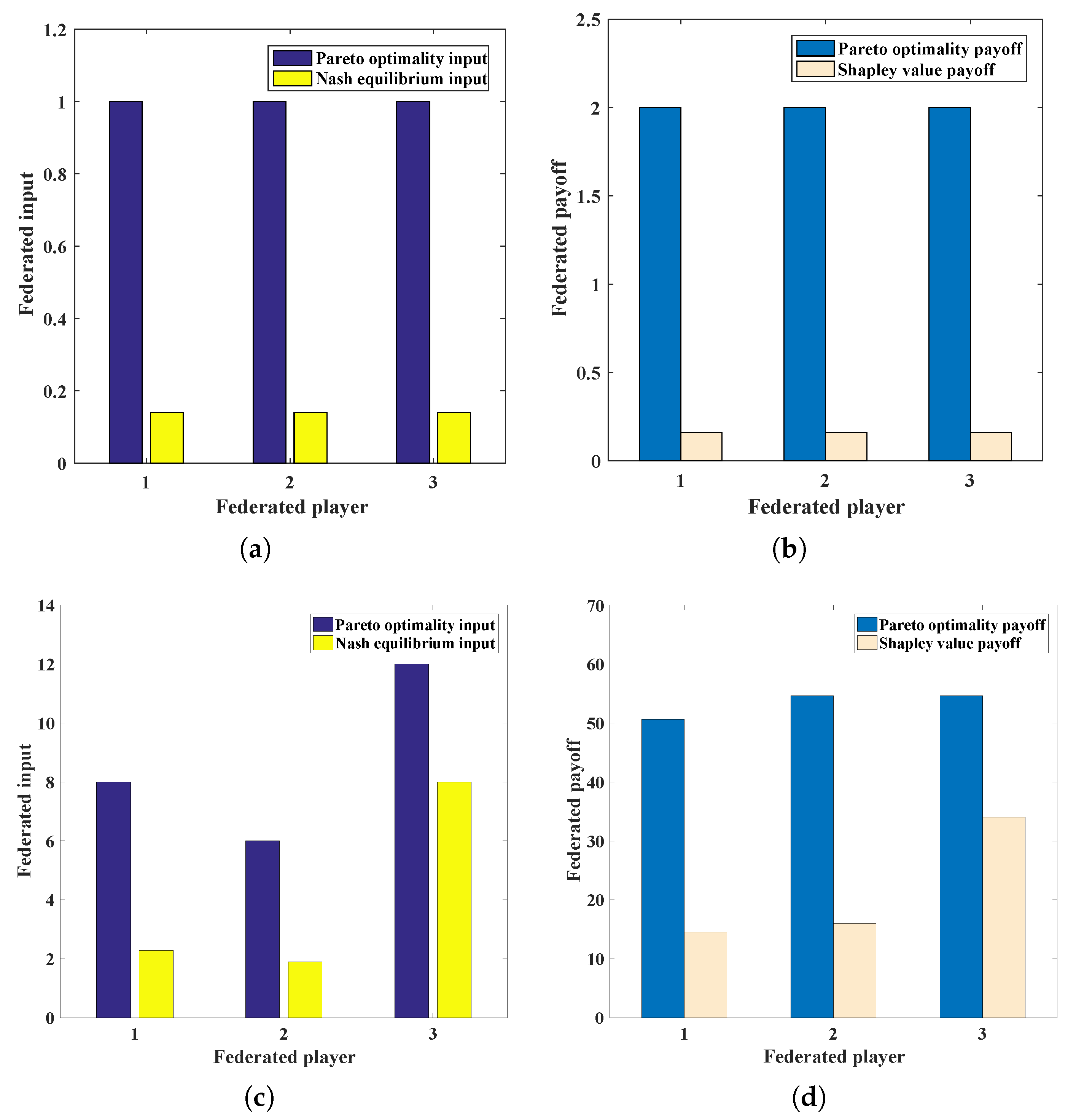
5.1. Numerical Example 1: Equal Status of Federated Players

Assuming there are three players in the FL system, and the federated payoff function is v ( x 1 , x 2 , x 3 ) = x 1 + x 2 + x 3 + x 1 x 2 + x 1 x 3 + x 2 x 3 , and the return function v ( x 1 , x 2 , x 3 ) is a strictly monotonically increasing concave function, the cost functions of the three players are c 1 ( x 1 ) = 3 2 x 1 2 , c 2 ( x 2 ) = 3 2 x 2 2 , and c 3 ( x 3 ) = 3 2 x 3 2 . It is easy to know that the cost function c i ( x i ) is a strictly increasing convex function. When the federated input is x * = ( x 1 * , x 2 * , x 3 * ) , the federated profit
max R = v ( x 1 , x 2 , x 3 ) i = 1 3 c i ( x i )
maximizes and satisfies Pareto optimality, and its first-order condition is
1 + x 2 * + x 3 * 3 x 1 * = 0 1 + x 1 * + x 3 * 3 x 2 * = 0 1 + x 1 * + x 2 * 3 x 3 * = 0
We determine that the federated inputs satisfying the Pareto optimality conditions are x 1 * = 1 , x 2 * = 1 , and x 3 * = 1 , the federated profit is v ( x * ) = 6 , and maximum profit is max R * = 1.5 . Because of the equal status of the three players, according to the anonymity of Formulas (6) and (7), the effectiveness of Formulas (6) and (7) can be obtained as
φ 1 ( v ( x ) ) = φ 2 ( v ( x ) ) = φ 3 ( v ( x ) ) φ 1 ( v ( x ) ) + φ 2 ( v ( x ) ) + φ 3 ( v ( x ) ) = v ( x ) φ 1 ( v ( x ) ) = φ 2 ( v ( x ) ) = φ 3 ( v ( x ) ) = 1 3 v ( x ) .
Therefore, the profit functions of the three players are
π 1 ( 1 3 v , x 1 ) = 1 3 v ( x ) 3 2 x 1 2 π 2 ( 1 3 v , x 2 ) = 1 3 v ( x ) 3 2 x 2 2 π 3 ( 1 3 v , x 3 ) = 1 3 v ( x ) 3 2 x 3 2 .
The Nash equilibrium requires other players to decide their investment in the FL, and each player has the right to decide their investment to maximize their profits. Therefore, the first-order condition that satisfies the Nash equilibrium is
1 + x 2 + x 3 9 x 1 = 0 1 + x 1 + x 3 9 x 2 = 0 1 + x 1 + x 2 9 x 3 = 0
We determine that the federated input satisfying the Nash equilibrium conditions are x ˜ 1 = 0.14 , x ˜ 2 = 0.14 , and x ˜ 3 = 0.14 , the federated payoff is v ( x ˜ ) = 0.49 and the maximum profit is max R ˜ = 0.4 .
By comparing the Pareto optimality solution and Nash equilibrium solution in Table 1, we know that using the Shapley value method can achieve fairness post-FL; the optimality incentive is not reached before FL. Under the Nash equilibrium, the input of each player is lower than the Pareto optimality level, and the federated profit cannot reach the maximum.
Next, we introduce the supervisory authority. If the supervisory authority knows that the federated payoff is greater than or equal to Pareto optimality payoff 6, the payoff is allocated to the federated players by Formulas (6) and (7). If it knows that the federated payoff is lower than Pareto optimality payoff 6, the payoff of the federated players is 0. The specific expression is as follows:
φ i ( v ( x ) ) = 1 3 v ( x ) , i f v ( x ) 6 , 0 , i f v ( x ) < 6 .
Here, we prove that the Nash equilibrium constituting the supervision mechanism satisfies the Pareto optimality condition x * = ( x 1 * , x 2 * , x 3 * ) = ( 1 , 1 , 1 ) . If the Pareto optimality values of the players 2 and 3 are x 1 * = 1 and x 2 * = 1 , respectively, the federated payoff is v ( x ) = 3 + 3 x 3 . If the input of player 3 is x 3 < 1 , there is v ( x ) < 6 , at this time,
φ 3 ( v ( x ) ) = 0 , π 3 ( 0 , x 3 ) = 0 3 2 x 3 2 < 0 ,
so rational player 3 will not input x 3 < 1 . If the federated input of player 3 is x 3 > 1 , then v ( x ) > 6 and
φ 3 ( v ( x ) ) = 1 3 v ( x ) = 4 3 + 2 3 x 3 , π 3 ( x 3 ) = 4 3 + 2 3 x 3 3 2 x 3 2 .
when x 3 1 , then π 3 ( x 3 ) x 3 = 2 3 3 x 3 < 0 , obviously, π 3 ( φ 3 , x 3 ) is a monotonic decreasing function of x 3 on interval [ 1 , ) , and the profit of player 3 reaches the maximum at x 3 = 1 . Therefore, the Nash equilibrium constituting the supervision mechanism satisfies the Pareto optimality condition x * = ( x 1 * , x 2 * , x 3 * ) = ( 1 , 1 , 1 ) .
Next, we consider the minimum value of penalty mechanism k i = φ i ( x ) π i ( x * ) . If the supervisory authority knows that the federated payoff is greater than or equal to Pareto optimality payoff 6, the payoff is allocated to the federated players by Formulas (6) and (7). If it knows that the federated payoff is lower than Pareto optimality payoff 6, the payoff of the federated players is 0.5. The specific expression is as follows:
φ i ( v ( x ) ) = 1 3 v ( x ) , i f v ( x ) 6 , 0.5 , i f v ( x ) < 6 .
Here, we prove that the Nash equilibrium constituting the supervision mechanism satisfies the Pareto optimality condition x * = ( x 1 * , x 2 * , x 3 * ) = ( 1 , 1 , 1 ) . If the Pareto optimality values of players 2 and 3 are x 1 * = 1 and x 2 * = 1 , respectively, the federated payoff is v ( x ) = 3 + 3 x 3 . If the input of player 3 is x 3 < 1 , there is v ( x ) < 6 . At this time,
φ 3 ( v ( x ) ) = 0.5 , π 3 ( 0 , x 3 ) = 0.5 3 2 x 3 2 0.5 ,
so rational player 3 will not input x 3 < 1 . If the federated input of player 3 is x 3 1 , then v ( x ) 6 and
φ 3 ( v ( x ) ) = 1 3 v ( x ) = 4 3 + 2 3 x 3 , π 3 ( x 3 ) = 4 3 + 2 3 x 3 3 2 x 3 2 .
In the last part, we proved that π 3 ( φ 3 , x 3 ) is a monotonic decreasing function of x 3 on interval [ 1 , ) , and the profit of player 3 reaches the maximum at x 3 = 1 .
According to the above, when x 1 * = 1 , x 2 * = 1 , and the input of player 3 is x 3 * = 1 , it just reaches the Pareto optimality value. At this time, π 3 ( x 3 * ) = 0.5 . Therefore, the condition to reach the Nash equilibrium of the mechanism is that the Pareto optimality input is x * = ( x 1 * , x 2 * , x 3 * ) = ( 1 , 1 , 1 ) .

5.2. Numerical Example 2: Unequal Status of Federated Players

Assuming that there are three federated players that form a coalition, and the federated payoff function is
v ( x 1 , x 2 , x 3 ) = 2 x 1 + 4 x 2 + 6 x 3 + x 1 x 2 .
The payoff function v ( x 1 , x 2 , x 3 ) is a strictly increasing linear function, and the cost functions c ( x 1 ) = 1 2 x 1 2 , c ( x 2 ) = x 2 2 and c ( x 3 ) = 1 4 x 3 2 of these three players are strictly monotonically increasing convex functions. When the federated input x * = ( x 1 * , x 2 * , x 3 * ) , the federated profit
max R = v ( x 1 , x 2 , x 3 ) i = 1 3 c i ( x i ) = 2 x 1 + 4 x 2 + 6 x 3 + x 1 x 2 1 2 x 1 2 x 2 2 1 4 x 3 2
maximizes and satisfies Pareto optimality, its first-order condition is
2 x 1 * + x 2 * = 0 4 + x 1 * 2 x 2 * = 0 6 1 2 x 3 * = 0 .
we determine that the federated inputs satisfying the Pareto optimality conditions are x 1 * = 8 , x 2 * = 6 , and x 3 * = 12 , the federated payoff is v ( x * ) = 160 , and the maximum profit is max R * = 56 . According to Formulas (6) and (7), because v ( 0 ) = 0 , v ( x 1 ) = 2 x 1 , v ( x 2 ) = 4 x 2 , v ( x 3 ) = 6 x 3 , v ( x 1 , x 2 ) = x 1 x 2 , v ( x 1 , x 3 ) = v ( x 2 , x 3 ) = 0 , and v ( x 1 , x 2 , x 3 ) = 2 x 1 + 4 x 2 + 6 x 3 + x 1 x 2 , then
φ 1 ( v ( x ) ) = 4 3 x 1 + 2 3 x 2 + x 3 + 1 2 x 1 x 2 φ 2 ( v ( x ) ) = 1 3 x 1 + 8 3 x 2 + x 3 + 1 2 x 1 x 2 φ 3 ( v ( x ) ) = 1 3 x 1 + 2 3 x 2 + 4 x 3 .
Therefore, the profit functions of the three players are
π 1 ( v , x 1 ) = 4 3 x 1 + 2 3 x 2 + x 3 + 1 2 x 1 x 2 1 2 x 1 2 π 2 ( v , x 2 ) = 1 3 x 1 + 8 3 x 2 + x 3 + 1 2 x 1 x 2 x 2 2 π 3 ( v , x 3 ) = 1 3 x 1 + 2 3 x 2 + 4 x 3 1 4 x 3 2 .
Nash equilibrium requires other players to decide their investment in the FL, and each player has the right to decide their investment, to maximize their profits. Therefore, the first-order condition satisfying Nash equilibrium is
4 3 x 1 + 1 2 x 2 = 0 8 3 + 1 2 x 1 2 x 2 = 0 4 1 2 x 3 = 0 .
we determine that the federated inputs satisfying the Pareto optimality conditions are x 1 = 2.29 , x 2 = 1.90 , and x 3 = 8 , the federated profit is v ( x ) = 64.53 , and the maximum profit is max R = 42.30 .
Comparing Pareto optimality and the Nash equilibrium solution in Table 2, we know that using the Shapley value method can achieve post fairness, but there is no prior optimality incentive. Under the Nash equilibrium, the input of each player is lower than the Pareto optimality level, and the federated profit does not reach the maximum.
Next, we introduce the supervisory authority. If the supervisory authority knows that the federated payoff is greater than or equal to the Pareto optimality payoff 160, the payoff is allocated to the federated players by Formulas (6) and (7). If it knows that the federated payoff is lower than Pareto optimality payoff 160, the federated player payoff is τ i . When the input of players reaches the Pareto optimality value, i.e., x 1 * = 8 , x 2 * = 6 , and x 3 * = 12 , then
φ 1 ( v ( x * ) = 4 3 x 1 * + 2 3 x 2 * + x 3 * + 1 2 x 1 * x 2 * = 50.67 φ 2 ( v ( x * ) = 1 3 x 1 * + 8 3 x 2 * + x 3 * + 1 2 x 1 * x 2 * = 54.67 φ 3 ( v ( x * ) = 1 3 x 1 * + 2 3 x 2 * + 4 x 3 * = 54.67 π 1 ( x * ) = 18.67 π 2 ( x * ) = 18.67 π 3 ( x * ) = 18.67 .
Therefore, the value ranges of τ 1 , τ 2 and τ 3 are 0 τ 1 18.67 , 0 τ 2 18.67 and 0 τ 3 18.67 , respectively. The payoffs φ 1 ( v ( x ) ) , φ 2 ( v ( x ) ) and φ 3 ( v ( x ) ) of players 1, 2 and 3 are as follows:
φ 1 ( v ( x ) ) = 4 3 x 1 + 2 3 x 2 + x 3 + 1 2 x 1 x 2 , i f v ( x ) 160 τ 1 , i f v ( x ) < 160
φ 2 ( v ( x ) ) = 1 3 x 1 + 8 3 x 2 + x 3 + 1 2 x 1 x 2 , i f v ( x ) 160 τ 2 , i f v ( x ) < 160
φ 3 ( v ( x ) ) = 1 3 x 1 + 2 3 x 2 + 4 x 3 , i f v ( x ) 160 τ 3 , i f v ( x ) < 160 .
In further work, we will prove that the Nash equilibrium constituting the supervision mechanism satisfies the Pareto optimality condition x * = ( x 1 * , x 2 * , x 3 * ) = ( 8 , 6 , 12 ) .
(1) We consider the value of player 1. When x 2 * = 6 and x 3 * = 12 , then
φ 1 ( v ( x ) ) = 13 3 x 1 + 16 , i f v ( x ) 8 τ 1 , i f v ( x ) < 8 .
where 0 τ 1 18.67 , and if the input of player 1 is x 1 8 , there is v 1 ( x ) = 13 3 x 1 + 16 , π 1 ( x ) = 13 3 x 1 + 16 1 2 x 1 2 , then π 1 ( x 1 ) x 1 = 13 3 x 1 < 0 . It indicates that the profit function π 1 ( x ) of player 1 is monotonically decreasing on [ 8 , ) ; therefore, when player 1 invests x 1 = 8 , it can obtain the maximum profit π 1 ( x ) = 18.67 . If player 1 invests x 1 < 8 , the player payoff is τ 1 and profit is π 1 ( x ) = τ 1 1 2 x 1 2 , then π 1 ( x ) = τ 1 1 2 x 1 2 18.67 . Thus, when x 2 * = 6 and x 3 * = 12 , player 1 can obtain the maximum profit π 1 ( x ) = 18.67 by investing x 1 * = 8 .
(2) We consider the value of player 2. When x 1 * = 8 and x 3 * = 12 , then
φ 2 ( v ( x ) ) = 20 3 x 2 + 44 3 , i f v ( x ) 6 τ 2 , i f v ( x ) < 6 .
where 0 τ 2 18.67 , and if the input of player 2 is x 2 6 , there is v 2 ( x ) = 20 3 x 2 + 44 3 and π 2 ( x ) = 20 3 x 2 + 44 3 x 2 2 , then π 2 ( x 2 ) x 2 = 20 3 2 x 2 < 0 . It indicates that the profit function π 2 ( x ) of player 2 is monotonically decreasing on [ 6 , ) ; therefore, when player 2 invests x 2 = 6 , it can obtain the maximum profit π 2 ( x ) = 18.67 . If player 2 invests x 1 < 6 , the player payoff is τ 2 and profit is π 2 ( x ) = τ 2 x 2 2 , then π 2 ( x ) = τ 2 x 2 2 18.67 . Thus, when x 1 * = 8 and x 3 * = 12 , player 2 can obtain the maximum profit π 2 ( x ) = 18.67 by investing x 2 = 6 .
(3) We consider the value of player 3. When x 1 * = 8 and x 2 * = 6 , then
φ 3 ( v ( x ) ) = 4 x 3 + 20 3 , i f v ( x ) 12 τ 3 , i f v ( x ) < 12 .
where 0 τ 3 18.67 , and if the input of player 3 is x 3 12 , there is v 3 ( x ) = 4 x 3 + 20 3 , π 3 ( x ) = 4 x 3 + 20 3 1 4 x 3 2 , then π 3 ( x 3 ) x 3 = 4 1 2 x 3 < 0 . It indicates that the profit function π 3 ( x ) of player 3 is monotonically decreasing on [ 12 , ) ; therefore, when player 3 invests x 3 = 12 , it can obtain the maximum profit π 3 ( x ) = 18.67 . If player 1 invests x 1 < 12 , player payoff is τ 3 and profit is π 3 ( x ) = τ 3 1 4 x 3 2 , then π 3 ( x ) = τ 3 1 4 x 3 2 12 . Thus, when x 1 * = 8 and x 2 * = 6 , player 3 can obtain the maximum profit π 3 ( x ) = 18.67 by investing x 3 = 12 .

5.3. Numerical Simulation Experiments

Figure 3 shows the simulations of numerical experiments 1 and 2, respectively. Subplot (a) and subplot (c) in Figure 3 show that the optimality inputs of the federated players have reached the Pareto optimality, and satisfying the Nash equilibrium’s inputs does not reach the Pareto optimality. Subplots (b) and (d) show that the payoffs of satisfying the Pareto optimality inputs are more than the federal payoffs of satisfying the Nash equilibrium inputs.
As in the literature [17,19], although the Shapley value method can satisfy the fair distribution of payoffs after FL, it cannot achieve Pareto efficiency optimality before FL, i.e., it cannot reach the optimality incentives for federated player inputs before FL, and neither individual nor collective maximum payoffs are achieved.
Therefore, according to the supervisory organization introduced in this paper, all federated players are observed to have lower federated payoffs than those satisfying the Pareto optimality, and the penalty goes to the supervisory organization. In this way, the supervisory organization supervises and disciplines all federated players.
By analyzing and proving that the inputs that satisfy the Pareto efficiency optimality constitute a Nash equilibrium for FL through the introduced supervisory organization, it is possible to solve the conflict that the payoff allocation of FL is fair and efficient.

6. Conclusions and Future Work

In the model training of FL, to obtain an accurate federated model, this paper designs an incentive mechanism to encourage all federated players to contribute to their data-training model. Under the condition of payoff determination, combined with the Shapley value method, a federated payoff allocation mechanism with third-party supervision is introduced. Under this mechanism, the federated payoff can reach Pareto optimality, and finally, the federated payoff is allocated by the Shapley value method. This mechanism solves the conflict between the fairness and efficiency of the payoff allocation in the FL system. Through the verification of numerical and simulation experiments, when the optimality payoff allocation of Pareto optimality is achieved, the Nash equilibrium of the mechanism is formed. Therefore, the use of an incentive mechanism will play a better role for federated players.
In future research, we apply the incentive mechanism solution proposed in this paper to solve the problem of payoff allocation among players in the training scenario of the FL model. In particular, the incentive mechanism proposed in this paper can be applied to banks, hospitals, insurance companies, etc., providing important theoretical assistance for them to train accurate federated models and improve economic efficiency in practice.

7. Discussion

The Shapley value method is a way to measure how much each player contributes to FL, and it is a fair rule for allocating resources. Pareto efficiency is a resource allocation’s ideal state, in which all resources are in full use and there is no waste. Although the Shapley value method can achieve fair payoff allocation after the completion of FL, it cannot guarantee that the inputs of each federated player achieve optimality before FL.
Therefore, the combination of the Shapley value and Pareto optimality provides a solution for federated payoff distribution that is both fair and efficient, and the solution can help ensure the stability and dynamic equilibrium of the payoff distribution.
However, this combination may have some shortcomings. For example, calculating the Shapley values in federated model training can be very complicated in the case of a large number of players. Furthermore, to determine the distribution of Pareto efficiency, the utility functions of all federated payers must be provided, which may be difficult to implement in practical applications.

Author Contributions

Conceptualization, X.Y. and S.X.; methodology, X.Y., S.X. and C.P.; software, X.Y. and S.X.; validation, X.Y., S.X., C.P. and Z.L.; writing—original draft preparation, X.Y.; writing review and editing, X.Y., W.T. and Z.L.; visualization, X.Y., C.P. and W.T.; supervision, X.Y., S.X., C.P. and N.W.; project administration, N.W. and Y.Z.; funding acquisition, Z.L. and Y.Z. All authors have read and agreed to the published version of the manuscript.

Funding

This work is supported by the National Natural Science Foundation of China (No. 62272124), the National Key Research and Development Program of China (No. 2022YFB2701401), the Guizhou Science Contract Plat Talent (No. [2020]5017), the Open Fund of Key Laboratory of Advanced Manufacturing Technology, Ministry of Education (grant No. GZUAMT2021KF[01]), the Research Project of Guizhou University for Talent Introduction (No. [2020]61), the Cultivation Project of Guizhou University (No. [2019]56), the Research Project of Guizhou University for Talent Introduction (GDRJHZ[2022]14), and Guizhou Provincial Science and Technology Projects (ZK[2023]YB053).

Data Availability Statement

The datasets used and/or analyzed in the current study are available from the corresponding author on reasonable request.

Acknowledgments

The authors are grateful to the referees for their careful reading of the manuscript and valuable comments. The authors thank the editor too.

Conflicts of Interest

The authors declare no conflict of interest.

Abbreviations

NThe set of n players
DThe set of players’ local dataset
MThe model trained jointly by all players
M F E D The FL sharing model
M S U M The traditional machine learning model
V F E D The model accuracy of M F E D
M S U M The model accuracy of M S U M
SThe alliance subset of different players, S N
v ( . ) A characteristic function
v ( S ) The player’s payoff through the alliance S
v ( N ) The overall federated payoff
φ i ( v ) The payoff allocated to player i
| S | The number of players in subset S
( | S | 1 ) ! The sorted total number when players i participates in coalition S
( n | S | ) ! The sorted total number of remaining ( n | S | ) players
S i The alliance after removing player i from alliance S
[ v ( S ) v ( S i ) ] The marginal contribution of i to coalition S
w ( | S | ) The weight coefficient
xA feasible action space
π ( x ) The federated player’s payoff function
c ( x ) The coalition cost input of player
k i The penalty condition for the supervisor to achieve Pareto optimality
r i ( x ) The supervisor obtained fines
RThe federated player’s profit

Appendix A

Appendix A.1. Proof of Theorem 1

Proof. 
According to the validity of the Shapley value, we can obtain
i = 1 n φ i ( v ) = v , v
By differentiating Formula (A1) with respect to x, we obtain
i = 1 n φ i ( v ) = 1 .
where φ i ( v ) = φ i / v , from the Nash equilibrium, assuming that the input of each federated player i is x i and the profit is π i ( φ i , x i ) = φ i ( v ) c i ( x i ) . The profit maximization of player i is
max π i ( φ i , x i ) = φ i ( v ) c i ( x i ) , i = 1 , 2 , , n
Therefore, the first-order condition of the Nash equilibrium is
φ i ( x ) x i = c i , i = 1 , 2 , , n .
Here, φ i ( x ) = φ i / x , x i = x / y i , and c i = c i / y i . To maximize federated profits, the federated investment needs to meet Pareto optimality:
y * = arg max y x ( y ) i = 1 n c i y i
the first-order condition of Pareto optimality is
x i = c i , i = 1 , 2 , , n .
In combination with Formulas (A4) and (A6), it can be seen that the Nash equilibrium achieves Pareto optimality, which only needs to satisfy the following conditions:
φ i ( x ) = 1 , i = 1 , 2 , , n
However, this is in contradiction to satisfying Shapley value condition i = 1 n φ i ( x ) = 1 . □

Appendix A.2. Proof of Theorem 2

Proof. 
To make the proof meaningful, we assume that when the federated players achieve Pareto optimality, the federated payoffs allocated by each player i according to the Shapley value method are greater than their input costs, i.e., v ( x i * ) > c i ( x i * ) . If x * = ( x 1 * , x 2 * , , x n * ) is the Nash equilibrium of this mechanism, it should satisfy π i [ v ( x i * , x n i * ) ] π i [ v ( x i , x n i * ) ] and
φ i ( v * ) c i ( x i * ) φ i ( v ) k i c i ( x i ) k i [ φ i ( v ) c i ( x i ) ] [ φ i ( v * ) c i ( x i * ) ]
During the FL process, the coalition input c i ( x i ) is invisible, and the value is not unique, so Formula (A8) cannot be used as a basis for formulating fines, but more importantly c i ( x i ) 0 , so there is φ i ( v ) [ φ i ( v * ) c i ( x i * ) ] [ φ i ( v ) c i ( x i ) ] [ φ i ( v * ) c i ( x i * ) ] . Therefore, Formula (A8) is only satisfied if the condition k i φ i ( v ) [ φ i ( v * ) c i ( x i * ) ] is satisfied so that the Pareto optimality value is achieved. The penalty condition for the supervisor to achieve Pareto optimality is
k i φ i ( v ) [ φ i ( v * ) c i ( x i * ) ]
However, to increase the players’ enthusiasm, it should be noted that fines should not be too high, and the principles of limited participation and limited liability are followed. Here, we assume that all players in federated learning are only responsible for limited liability. The amount of the penalty cannot exceed the amount of the player’s payoff, so if the player’s payoff is zero, there is no need for a penalty. Therefore, according to Formula (8), φ i ( v ) k i 0 is obtained, then
k i φ i ( v ) .
According to Formulas (A9) and (A10), we obtain
φ i ( v ) [ φ i ( v * ) c i ( x i * ) ] k i φ i ( v ) .
Assuming that the net payoff of player i after being fined is δ i , then δ i = φ i ( v ) k i , and the following formula can be obtained according to Formula (A11):
0 δ i φ i ( v * ) c i ( x i * )
According to the above, under the constraint of limited liability, the Pareto value is optimized. When the penalty of the supervisor meets Formula (A11), the optimality mechanism is
r i ( x ) = φ i ( v ) , i f v v ( x * ) δ i , i f v < v ( x * )
where the value of δ i satisfies Formula (A12), i = 1 , 2 , , n . Next, we explain the mechanism under two conditions of the penalty value in Formula (A12).
When k i = φ i ( v ) , it means that the supervisor knows that the federated payoff is greater than or equal to the Pareto optimality payoff, and the supervisor will distribute the federated payoff to all players according to the Shapley value formula. If the federated payoff is less than the Pareto optimality payoff, all federated payoffs will belong to the supervisor. The expression is
r i ( x ) = φ i ( v ) , i f v v ( x * ) 0 , i f v < v ( x * )
Furthermore, we will prove that the federated input x * = ( x 1 * , x 2 * , , x n * ) satisfying Pareto optimality is the Nash equilibrium of this mechanism.
Assuming that the federated input of player i is x i < x * and the federated input of other players is x n i * because v ( x ) is a monotonically increasing function, then v ( x i , x n i * ) < v ( x i * , x n i * ) , r i ( x i , x n i * ) = 0 , and the profit of player i is π i ( x i ) = c i ( x i ) 0 ; therefore, rational player i will not invest x i < x * . If the federated input of player i is x i x * and because v ( x ) is a monotonically increasing function, then the profit of player i is π i ( x i ) = φ i ( x i ) c i ( x i ) > 0 ; therefore, rational player i will invest x i x * . □

References

  1. Konečnỳ, J.; McMahan, H.B.; Ramage, D.; Richtárik, P. Federated optimization: Distributed machine learning for on-device intelligence. arXiv 2016, arXiv:1610.02527. [Google Scholar]
  2. McMahan, H.B.; Moore, E.; Ramage, D.; y Arcas, B.A. Federated learning of deep networks using model averaging. arXiv 2016, arXiv:1602.05629. [Google Scholar]
  3. Konečnỳ, J.; McMahan, H.B.; Yu, F.X.; Richtárik, P.; Suresh, A.T.; Bacon, D. Federated learning: Strategies for improving communication efficiency. arXiv 2016, arXiv:1610.05492. [Google Scholar]
  4. Yang, Q.; Liu, Y.; Chen, T.; Tong, Y. Federated machine learning: Concept and applications. ACM Trans. Intell. Syst. Technol. (TIST) 2019, 10, 1–19. [Google Scholar] [CrossRef]
  5. Kairouz, P.; McMahan, H.B.; Avent, B.; Bellet, A.; Bennis, M.; Bhagoji, A.N.; Bonawitz, K.; Charles, Z.; Cormode, G.; Cummings, R.; et al. Advances and open problems in federated learning. Found. Trends® Mach. Learn. 2021, 14, 1–210. [Google Scholar] [CrossRef]
  6. Sarikaya, Y.; Ercetin, O. Motivating workers in federated learning: A stackelberg game perspective. IEEE Netw. Lett. 2019, 2, 23–27. [Google Scholar] [CrossRef] [Green Version]
  7. Zhan, Y.; Li, P.; Qu, Z.; Zeng, D.; Guo, S. A learning-based incentive mechanism for federated learning. IEEE Internet Things J. 2020, 7, 6360–6368. [Google Scholar] [CrossRef]
  8. Kang, J.; Xiong, Z.; Niyato, D.; Xie, S.; Zhang, J. Incentive mechanism for reliable federated learning: A joint optimization approach to combining reputation and contract theory. IEEE Internet Things J. 2019, 6, 10700–10714. [Google Scholar] [CrossRef]
  9. Tran, N.H.; Bao, W.; Zomaya, A.; Nguyen, M.N.; Hong, C.S. Federated learning over wireless networks: Optimization model design and analysis. In Proceedings of the IEEE INFOCOM 2019-IEEE Conference on Computer Communications, Paris, France, 29 April–2 May 2019; IEEE: Piscataway, NJ, USA, 2019; pp. 1387–1395. [Google Scholar]
  10. Yu, H.; Liu, Z.; Liu, Y.; Chen, T.; Cong, M.; Weng, X.; Niyato, D.; Yang, Q. A fairness-aware incentive scheme for federated learning. In Proceedings of the AAAI/ACM Conference on AI, Ethics, and Society, New York, NY, USA, 7–8 February 2020; Volume 2020, pp. 393–399. [Google Scholar]
  11. Li, T.; Sanjabi, M.; Beirami, A.; Smith, V. Fair resource allocation in federated learning. arXiv 2019, arXiv:1905.10497. [Google Scholar]
  12. Holmstrom, B. Moral hazard in teams. Bell J. Econ. 1982, 13, 324–340. [Google Scholar] [CrossRef]
  13. Kim, H.; Park, J.; Bennis, M.; Kim, S.L. Blockchained on-device federated learning. IEEE Commun. Lett. 2019, 24, 1279–1283. [Google Scholar] [CrossRef] [Green Version]
  14. Feng, S.; Niyato, D.; Wang, P.; Kim, D.I.; Liang, Y.C. Joint service pricing and cooperative relay communication for federated learning. In Proceedings of the 2019 International Conference on Internet of Things (iThings) and IEEE Green Computing and Communications (GreenCom) and IEEE Cyber, Physical and Social Computing (CPSCom) and IEEE Smart Data (SmartData), Atlanta, GA, USA, 14–17 July 2019; IEEE: Piscataway, NJ, USA, 2019; pp. 815–820. [Google Scholar]
  15. Yang, X. An exterior point method for computing points that satisfy second-order necessary conditions for a C1, 1 optimization problem. J. Math. Anal. Appl. 1994, 187, 118–133. [Google Scholar] [CrossRef] [Green Version]
  16. Wang, Z.; Hu, Q.; Li, R.; Xu, M.; Xiong, Z. Incentive mechanism design for joint resource allocation in blockchain-based federated learning. IEEE Trans. Parallel Distrib. Syst. 2023, 34, 1536–1547. [Google Scholar] [CrossRef]
  17. Song, T.; Tong, Y.; Wei, S. Profit allocation for federated learning. In Proceedings of the 2019 IEEE International Conference on Big Data (Big Data), Los Angeles, CA, USA, 9–12 December 2019; IEEE: Piscataway, NJ, USA, 2019; pp. 2577–2586. [Google Scholar]
  18. Wang, T.; Rausch, J.; Zhang, C.; Jia, R.; Song, D. A principled approach to data valuation for federated learning. In Federated Learning: Privacy and Incentive; Springer: Cham, Switzerland, 2020; pp. 153–167. [Google Scholar]
  19. Wang, G.; Dang, C.X.; Zhou, Z. Measure contribution of participants in federated learning. In Proceedings of the 2019 IEEE International Conference on Big Data (Big Data), Los Angeles, CA, USA, 9–12 December 2019; IEEE: Piscataway, NJ, USA, 2019; pp. 2597–2604. [Google Scholar]
  20. Liu, Y.; Ai, Z.; Sun, S.; Zhang, S.; Liu, Z.; Yu, H. Fedcoin: A peer-to-peer payment system for federated learning. In Federated Learning: Privacy and Incentive; Springer: Berlin/Heidelberg, Germany, 2020; pp. 125–138. [Google Scholar]
  21. Zeng, R.; Zeng, C.; Wang, X.; Li, B.; Chu, X. A comprehensive survey of incentive mechanism for federated learning. arXiv 2021, arXiv:2106.15406. [Google Scholar]
  22. Liu, Z.; Chen, Y.; Yu, H.; Liu, Y.; Cui, L. Gtg-shapley: Efficient and accurate participant contribution evaluation in federated learning. ACM Trans. Intell. Syst. Technol. (TIST) 2022, 13, 1–21. [Google Scholar] [CrossRef]
  23. Nagalapatti, L.; Narayanam, R. Game of gradients: Mitigating irrelevant clients in federated learning. In Proceedings of the AAAI Conference on Artificial Intelligence, Virtual, 2–9 February 2021; Volume 35, pp. 9046–9054. [Google Scholar]
  24. Fan, Z.; Fang, H.; Zhou, Z.; Pei, J.; Friedlander, M.P.; Liu, C.; Zhang, Y. Improving fairness for data valuation in horizontal federated learning. In Proceedings of the 2022 IEEE 38th International Conference on Data Engineering (ICDE), Kuala Lumpur, Malaysia, 9–12 May 2022; IEEE: Piscataway, NJ, USA, 2022; pp. 2440–2453. [Google Scholar]
  25. Fan, Z.; Fang, H.; Zhou, Z.; Pei, J.; Friedlander, M.P.; Zhang, Y. Fair and efficient contribution valuation for vertical federated learning. arXiv 2022, arXiv:2201.02658. [Google Scholar]
  26. Yang, X.; Tan, W.; Peng, C.; Xiang, S.; Niu, K. Federated Learning Incentive Mechanism Design via Enhanced Shapley Value Method. Wirel. Commun. Mob. Comput. 2022, 2022, 9690657. [Google Scholar] [CrossRef]
  27. McMahan, B.; Moore, E.; Ramage, D.; Hampson, S.; y Arcas, B.A. Communication-efficient learning of deep networks from decentralized data. In Proceedings of the Artificial Intelligence and Statistics, PMLR, Fort Lauderdale, FL, USA, 20–22 April 2017; pp. 1273–1282. [Google Scholar]
  28. Shapley, L.S. A value for n-person games. Contrib. Theory Games 1953, 2, 307–317. [Google Scholar]
  29. Zhou, Z.H.; Yu, Y.; Qian, C. Evolutionary Learning: Advances in Theories and Algorithms; Springer: Berlin/Heidelberg, Germany, 2019. [Google Scholar]
  30. Pardalos, P.M.; Migdalas, A.; Pitsoulis, L. Pareto Optimality, Game Theory and Equilibria; Springer Science & Business Media: Berlin/Heidelberg, Germany, 2008; Volume 17. [Google Scholar]
  31. Nas, J. Non-cooperative games. Ann. Math. 1951, 54, 286–295. [Google Scholar] [CrossRef]
  32. Ye, M.; Hu, G. Distributed Nash Equilibrium Seeking by a Consensus Based Approach. IEEE Trans. Autom. Control 2017, 62, 4811–4818. [Google Scholar] [CrossRef] [Green Version]
  33. Alchian, A.A.; Demsetz, H. Production, information costs, and economic organization. Am. Econ. Rev. 1972, 62, 777–795. [Google Scholar]
Figure 1. Federated learning framework.
Axioms 12 00636 g001
Figure 2. Federated learning incentive model.
Axioms 12 00636 g002
Figure 3. Federated player’s input and payoff comparison. (a) Example 1: Federated player’s input. (b) Example 1: Federated player’s payoff. (c) Example 2: Federated player’s input. (d) Example 2: Federated player’s payoff.
Axioms 12 00636 g003
Table 1. Example 1: Federated input and profit comparison.
Input and Profit ComparisonInput x 1 Input x 2 Input x 3 Federated ProfitMaximum Profit
Pareto optimality11161.5
Nash equilibrium0.140.140.140.490.4
Table 2. Example 2: Federated input and profit comparison.
Input and Profit ComparisonInput x 1 Input x 2 Input x 3 Federated ProfitMaximum Profit
Pareto optimality861216056
Nash equilibrium2.191.90864.5342.30
Disclaimer/Publisher’s Note: The statements, opinions and data contained in all publications are solely those of the individual author(s) and contributor(s) and not of MDPI and/or the editor(s). MDPI and/or the editor(s) disclaim responsibility for any injury to people or property resulting from any ideas, methods, instructions or products referred to in the content.

