Optimality Conditions of the Approximate Efficiency for Nonsmooth Robust Multiobjective Fractional Semi-Infinite Optimization Problems

Abstract

This paper is devoted to the investigation of optimality conditions and saddle point theorems for robust approximate quasi-weak efficient solutions for a nonsmooth uncertain multiobjective fractional semi-infinite optimization problem (NUMFP). Firstly, a necessary optimality condition is established by using the properties of the Gerstewitz’s function. Furthermore, a kind of approximate pseudo/quasi-convex function is defined for the problem (NUMFP), and under its assumption, a sufficient optimality condition is obtained. Finally, we introduce the notion of a robust approximate quasi-weak saddle point to the problem (NUMFP) and prove corresponding saddle point theorems.

1. Introduction

Recently, much attention had been paid to semi-infinite optimization problems; see [1,2,3]. Specially, multiobjective semi-infinite optimization refers to finding values of decision variables that give the optimum of more than one objective, and many interesting results have been presented in [4] and the references therein. Moreover, fractional optimization is a ratio of two functions, and it is widely used in the fields of information technology, resource allocation and engineering design; see [5,6,7,8]. It is worth noting that in many practical problems the objective or constraint functions to optimization models are nonsmooth and are affected by various uncertain information. Therefore, it is meaningful to investigate nonsmooth uncertain optimization problems; see [9,10,11]. Robust optimization [12,13] is one of the powerful tools to deal with optimization problems with data uncertainty. The aim of the robust optimization approach is to find the worst-case solution, which is immunized against the data uncertainty to optimization problems. However, most of solutions obtained by numerical algorithms are approximate solutions. In these situations, the study of approximate solutions is very significant from both the theoretical aspect and practical application. This paper intends to investigate the properties of a problem (NUMFP) with respect to approximate quasi-weak efficient solutions by the robust approach.

Optimality conditions and saddle point theorems are two important contents of nonsmooth optimization problems. The subdifferential is a powerful tool to characterize optimality conditions. For a nonsmooth multiobjective optimization problem, Caristi et al. [14] and Kabgani et al. [15] investigated optimality conditions of weakly efficient solutions by using the Michel–Penot subdifferential and convexificator, respectively. Chuong [5] obtained optimality theorems for robust efficient solutions to a nonsmooth multiobjective fractional optimization problem based on the Mordukhovich subdifferential. It is important to mention that the Clarke subdifferential has attracted much attention because of its good properties [16]. Fakhar et al. [17] constructed optimality conditions and saddle point theorems of robust efficient solutions for a nonsmooth multiobjective optimization problem by utilizing the Clarke subdifferential. The purpose of this article is to examine optimality conditions and saddle point theorems of robust approximate quasi-weak efficient solutions for a problem (NUMFP) under the Clarke subdifferential. Moreover, Lee et al. [18] employed a separation theorem to established necessary conditions for approximate solutions. Chen et al. [19] used a generalized alternative theorem to obtain necessary optimality conditions for weakly robust efficient solutions. It is worth noting that the Gerstewitz’s function is an important nonlinear scalar function, which plays a significant role in solving optimization problems due to its good properties, such as convexity, positive homogeneity and continuity; see [20,21]. This paper will use the Gerstewitz’s function to examine a necessary optimality condition of robust approximate quasi-weak efficient solutions for a problem (NUMFP).

In addition, convexity and its generalization play an important role in establishing sufficient optimality conditions of optimization problems. In this paper, we will define a class of approximate (pseudo quasi) convex functions for the objective and constraint functions of a problem (NUMFP) and establish a sufficient optimality condition and saddle point theorems for robust approximate quasi-weak efficient solutions under their assumptions.

This paper is organized as follows. Section 2 provides some basic concepts and lemmas, which will be used in the subsequent sections. In Section 3, we establish optimality conditions for robust approximate quasi-weak efficient solutions to a problem (NUMFP). In Section 4, we introduce the concept of a robust approximate quasi-weak saddle point to a problem (NUMFP) and prove corresponding saddle point theorems.

2. Preliminaries

Throughout this paper, $\mathbb{N}$ and ${\mathbb{R}}^n$ stand for the set of natural numbers and n-dimensional Euclidean space, respectively. $\mathbb{B}(\overline{x},r)$ denotes the open ball with center $\overline{x}\in {\mathbb{R}}^n$ and radius $r>0$; $\mathbb{B}$ represents the closed unit ball of ${\mathbb{R}}^n$. The inner product in ${\mathbb{R}}^n$ is denoted by $⟨x,y⟩$ for any $x,y\in {\mathbb{R}}^n$. We set

$$\begin{array}{c}\hfill {\mathbb{R}}_{+}^n=\{x=(x_1,\cdots ,x_n)\in {\mathbb{R}}^n\mid x_i\ge 0,i=1,\cdots ,n\},\end{array}$$

$${\mathbb{R}}_{++}^n=\{x=(x_1,\cdots ,x_n)\in {\mathbb{R}}^n\mid x_i>0,i=1,\cdots ,n\},$$

and utilize the following symbols to represent an order relation in ${\mathbb{R}}^n$:

$$x<y\iff y-x\in {\mathbb{R}}_{++}^n,$$

$$x\leqq y\iff y-x\in {\mathbb{R}}_{+}^n.$$

Let $C\subset {\mathbb{R}}^n$ be a nonempty subset and $\mathrm{int}C,\mathrm{cl}C$ and $\mathrm{co}C$ stand for the interior, the closure, and the convex hull of C, respectively. The Clarke contingent cone and normal cone to C at point $\overline{x}\in {\mathbb{R}}^n$ are defined, respectively, by the following (see [16]):

$$T(C,\overline{x})=\{y\in {\mathbb{R}}^n\mid \forall x_n\in C,x_n\to \overline{x},\forall t_n\to 0,\exists y_n\to y,s.t.x_n+t_n{y}_n\in C,\forall n\in \mathbb{N}\},$$

$$N(C,\overline{x})=\{\xi \in {\mathbb{R}}^n\mid ⟨\xi ,y⟩\le 0,\forall y\in T(C,\overline{x})\}.$$

The conical convex hull (see [22]) of the set C is defined as

$$pos(C)=\{y\in {\mathbb{R}}^n\mid \exists l\in \mathbb{N}s.t.y=\sum _{i=1}^l{\lambda }_i{y}_i,{\lambda }_i\ge 0,y_i\in C,i=1,\cdots ,l\}.$$

Let $F:{\mathbb{R}}^n\to {\mathbb{R}}^m$. F is said to be locally Lipschitz at $\overline{x}\in {\mathbb{R}}^n$ if there exist constant $L>0$ and $r>0$ such that

$$\Vert F(x_1)-F(x_2)\Vert \le L\Vert x_1-x_2\Vert ,\forall x_1,x_2\in \mathbb{B}(\overline{x},r).$$

If F is locally Lipschitz at x for any $x\in {\mathbb{R}}^n$, then F is called locally Lipschitz mapping. Particularly, for a real value locally Lipschitz function $f:{\mathbb{R}}^n\to \mathbb{R}$ ($\mathbb{R}$ denotes real number), the Clarke generalized directional derivative of f at $\overline{x}\in {\mathbb{R}}^n$ in the direction $d\in {\mathbb{R}}^n$ is given by (see [16])

$$f(\overline{x};d)=\underset{y\to \overline{x},t\to 0^{+}}{\lim \sup }\frac{f(y+td)-f(y)}{t},$$

and the Clarke subdifferential (see [16]) of f at $\overline{x}$ is denoted by

$$\partial f(\overline{x})=\{\xi \in {\mathbb{R}}^n\mid f(\overline{x};d)\ge ⟨\xi ,d⟩,\forall d\in {\mathbb{R}}^n\}.$$

Let $C\subset {\mathbb{R}}^n$ be a nonempty subset, and the indicator function of C is defined as

$$\begin{array}{c}\hfill {\delta }_C(x)=\left\{\begin{array}{c}0,x\in C,\hfill \\ +\infty ,x\notin C.\hfill \end{array}\right.\end{array}$$

It is pointed out in [16] that

$$\partial {\delta }_C(\overline{x})=N(C,\overline{x}),\forall \overline{x}\in C.$$

The following lemmas characterize some properties of the Clarke subdifferential.

Lemma 1

([16]). Let $f,h:{\mathbb{R}}^n\to \mathbb{R}$ be locally Lipschitz at $\overline{x}\in {\mathbb{R}}^n$. Then, the following applies:

(i)

$\partial f(\overline{x})$ is nonempty compact convex;

(ii)

for any $t\in \mathbb{R},\partial f(t\overline{x})=t\partial f(\overline{x});$

(iii)

$\partial (f+h)(\overline{x})\subset \partial f(\overline{x})+\partial h(\overline{x});$

(iv)

if f attains a local minimum at $\overline{x}$, then $0\in \partial f(\overline{x})$.

Lemma 2

([16]). Let $f,h:{\mathbb{R}}^n\to \mathbb{R}$ be locally Lipschitz at $\overline{x}\in {\mathbb{R}}^n$, and $h(\overline{x})\ne 0$. Then, $\frac{f}{h}$ is also locally Lipschitz at $\overline{x}$, and

$$\partial (\frac{f}{h})(\overline{x})\subset \frac{h(\overline{x})\partial f(\overline{x})-f(\overline{x})\partial h(\overline{x})}{{(h(\overline{x}))}^2}.$$

Lemma 3

([16]). Let $F:{\mathbb{R}}^n\to {\mathbb{R}}^m$ be locally Lipschitz at $\overline{x}\in {\mathbb{R}}^n$ and $f:{\mathbb{R}}^m\to \mathbb{R}$ be locally Lipschitz at $F(\overline{x})$. Then,

$$\partial (f\circ F)(\overline{x})\subset \mathrm{cl}(co(\bigcup _{\mathsf{\Lambda }\in \partial f(F(\overline{x}))}\partial (\mathsf{\Lambda }\circ F)(\overline{x}))).$$

Next, we give a scalar function, which will play an essential role in the proof of optimality conditions in Section 3.

Definition 1

([20]). Let $C\subset {\mathbb{R}}^n$ be a pointed closed convex cone, $\overline{e}\in intC\ne \varnothing$. The Gerstewitz’s function ${\Psi }_{\overline{e}}:{\mathbb{R}}^n\to \mathbb{R}$ is defined as

$${\Psi }_{\overline{e}}(y)=inf\{t\in \mathbb{R}\mid y\in t\overline{e}-C\},y\in {\mathbb{R}}^n.$$

Some properties of the Gerstewitz’s function are summarized in the following Lemma 4.

Lemma 4

([20]). Let $C\subset {\mathbb{R}}^n$ be a pointed closed convex cone, $\overline{e}\in \mathrm{int}C\ne \varnothing$. Then, the following applies:

(i)

${\Psi }_{\overline{e}}$ is continuous and locally a Lipschitz function;

(ii)

${\Psi }_{\overline{e}}(y)\le t\iff y\in t\overline{e}-C$;

(iii)

${\Psi }_{\overline{e}}(y)\ge t\iff y\notin t\overline{e}-\mathrm{int}C$;

(iv)

$\partial {\Psi }_{\overline{e}}(y)=\{\lambda \in C^{*}\mid ⟨\lambda ,y⟩={\Psi }_{\overline{e}}(y)\}$;

(v)

$\partial {\Psi }_{\overline{e}}(y)\subset C^{*}\backslash \{0\}$,

where $C^{*}=\{\lambda \in {\mathbb{R}}^n\mid ⟨\lambda ,y⟩\ge 0,\forall y\in C\}$ represents the dual cone of C.

Lemma 5

([22]). Let $\{C_i\mid i\in I\}$ be an arbitrary collection of nonempty convex sets in ${\mathbb{R}}^n$ and K be the convex cone generated by the union of the collection. Then, every nonzero vector of K can be expressed as a nonnegative linear combination of n or fewer linearly independent vectors, each belonging to a different $C_i$.

Let T be a nonempty and arbitrary index set. Considering the following nonsmooth uncertain multiobjective fractional semi-infinite optimization problem (NUMFP)

$$\begin{array}{c}\hfill (\mathrm{NUMFP})\left\{\begin{array}{c}min\frac{f(x)}{h(x)}=(\frac{f_1(x)}{h_1(x)},\cdots ,\frac{f_l(x)}{h_l(x)}),\hfill \\ \mathrm{s}.\mathrm{t}.g_t(x,v_t)\le 0,\forall t\in T,\hfill \end{array}\right.\end{array}$$

where $v_t\mathrm{and}t\in T$, are uncertain parameters from the uncertainty set $V_t\subset {\mathbb{R}}^p,t\in T$. $f_i,h_i:{\mathbb{R}}^n\to \mathbb{R},h_i(x)\ne 0,i=1,\cdots ,l$, $g_t:{\mathbb{R}}^n\times V_t\to \mathbb{R}$, $f_i,h_i,g_t$ are locally Lipschitz functions, and the uncertainty map $V:T\rightrightarrows {\mathbb{R}}^p$ is defined as $V(t):=V_t$.

We consider the robust counterpart of the problem (NUMFP) as follows:

$$\begin{array}{c}\hfill (\mathrm{NRMFP})\left\{\begin{array}{c}min\frac{f(x)}{h(x)}=(\frac{f_1(x)}{h_1(x)},\cdots ,\frac{f_l(x)}{h_l(x)}),\hfill \\ \mathrm{s}.\mathrm{t}.g_t(x,v_t)\le 0,\forall v_t\in V_t,t\in T,\hfill \end{array}\right.\end{array}$$

where the feasible set of the problem (NRMFP) is denoted by

$$\mathcal{F}:=\{x\in {\mathbb{R}}^n\mid g_t(x,v_t)\le 0,\forall v_t\in V_t,t\in T\}.$$

Definition 2.

Let $\epsilon =({\epsilon }_1,\cdots ,{\epsilon }_l)\in {\mathbb{R}}_{+}^l$. $\overline{x}\in \mathcal{F}$ is called a robust quasi-weak ε-efficient solution of the problem (NUMFP) if $\overline{x}$ is a quasi-weak ε-efficient solution of the problem (NRMFP); that is,

$$\frac{f(x)}{h(x)}-\frac{f(\overline{x})}{h(\overline{x})}+\epsilon \parallel x-\overline{x}\parallel \notin -{\mathbb{R}}_{++}^l,\forall x\in \mathcal{F}.$$

Remark 1.

When $\epsilon =0$, the quasi-weak ε-efficient solution degrades into the weak efficient solution in [8].

3. Optimality Conditions

In this section, we will establish necessary and sufficient optimality conditions for the quasi-weak $\epsilon$-efficient solutions to the problem (NRMFP). We begin with the following constraint qualification.

Definition 3

([23]). For $x\in {\mathbb{R}}^n$, let $\Pi (x):=\{(t,v)\in gphV\mid g_t(x,v)=0\}$ and

$$\Delta (x):=\bigcup _{(t,v)\in \Pi (x)}{\partial }_x{g}_t(x,v),$$

where $gphV:=\{(t,v)\in T\times {\mathbb{R}}^p\mid v\in V(t)\}$.

Definition 4

([16]). Let $\overline{x}\in \mathcal{F}$. The Basic Constraint Qualification (BCQ) holds at $\overline{x}$ if $N(\mathcal{F},\overline{x})\subset pos(\Delta (\overline{x}))$.

Next, we present a necessary optimality condition for the quasi-weak $\epsilon$-efficient solutions to the problem (NRMFP) by using the properties of the Gerstewitz’s function.

Theorem 1.

In problem (NRMFP), let $\epsilon =({\epsilon }_1,\cdots ,{\epsilon }_l)\in {\mathbb{R}}_{+}^l$. If $\overline{x}\in \mathcal{F}$ is a quasi-weak ε-efficient solution of the problem (NRMFP) and the BCQ holds at $\overline{x}$, then there exist $\overline{\alpha }=({\overline{\alpha }}_1,\cdots ,{\overline{\alpha }}_l)\in {\mathbb{R}}_{+}^l\backslash \{0\},{\overline{\lambda }}_i=\frac{{\overline{\alpha }}_i}{h_i(\overline{x})},i=1,\cdots ,l,\overline{\mu }=({\overline{\mu }}_1,\cdots ,{\overline{\mu }}_n)\in {\mathbb{R}}_{+}^n$ and $({\overline{t}}_j,{\overline{v}}_j)\in gphV,j=1,\cdots ,n$, such that

$$\begin{array}{c}\hfill 0\in \sum _{i=1}^l{\overline{\lambda }}_i(\partial f_i(\overline{x})-\frac{f_i(\overline{x})}{h_i(\overline{x})}\partial h_i(\overline{x}))+\sum _{j=1}^n{\overline{\mu }}_j{\partial }_x{g}_{{\overline{t}}_j}(\overline{x},{\overline{v}}_j)+\sum _{i=1}^l{\overline{\alpha }}_i{\epsilon }_i\mathbb{B},\end{array}$$

(1)

$$\begin{array}{c}\hfill {\overline{\mu }}_j{g}_{{\overline{t}}_j}(\overline{x},{\overline{v}}_j)=0,\forall j=1,\cdots ,n.\end{array}$$

(2)

Proof. 

Since $\overline{x}$ is a quasi-weak $\epsilon$-efficient solution of the problem (NRMFP), we obtain

$$\frac{f(x)}{h(x)}-\frac{f(\overline{x})}{h(\overline{x})}+\epsilon \parallel x-\overline{x}\parallel \notin -{\mathbb{R}}_{++}^l,\forall x\in \mathcal{F}.$$

Let $H(x)=(\frac{f(x)}{h(x)}-\frac{f(\overline{x})}{h(\overline{x})}+\epsilon \parallel x-\overline{x}\parallel )$, by Lemma 4 (iii), then we obtain

$$\begin{array}{c}\hfill {\Psi }_{(\overline{e})}(H(x))\ge 0,\forall x\in \mathcal{F}.\end{array}$$

As $\overline{x}\in \mathcal{F}$, thus,

$$\begin{array}{c}\hfill {\Psi }_{(\overline{e})}(H(\overline{x}))\ge 0.\end{array}$$

(3)

Note that $H(\overline{x})=0,$ then $H(\overline{x})\in -{\mathbb{R}}_{+}^l$, and it follows from Lemma 4 (ii) that

$$\begin{array}{c}\hfill {\Psi }_{(\overline{e})}(H(\overline{x}))\le 0,\end{array}$$

together with (3), and then we have

$$\begin{array}{c}\hfill {\Psi }_{(\overline{e})}(H(\overline{x}))=0.\end{array}$$

Therefore,

$$\begin{array}{c}\hfill {\Psi }_{(\overline{e})}(H(x))\ge {\Psi }_{(\overline{e})}(H(\overline{x}))=0,\forall x\in \mathcal{F},\end{array}$$

and this means that $\overline{x}$ is a local minimizer of ${\Psi }_{(\overline{e})}\circ H(x)$ on $\mathcal{F}$, and $\overline{x}$ is also a local minimizer of ${\Psi }_{(\overline{e})}\circ H(x)+{\delta }_{\mathcal{F}}(x)$ on $\mathcal{F}$. By Lemma 1 (iii), we obtain

$$\begin{array}{c}\hfill 0\in \partial ({\Psi }_{(\overline{e})}\circ H+{\delta }_{\mathcal{F}})(\overline{x})\subset \partial ({\Psi }_{(\overline{e})}\circ H)(\overline{x})+\partial {\delta }_{\mathcal{F}}(\overline{x}).\end{array}$$

(4)

Due to

$$\begin{array}{c}\hfill \partial {\delta }_{\mathcal{F}}(\overline{x})=N(\mathcal{F};\overline{x}),\end{array}$$

combined with (4), we arrive at

$$\begin{array}{c}\hfill 0\in \partial ({\Psi }_{(\overline{e})}\circ H)(\overline{x})+N(\mathcal{F};\overline{x}).\end{array}$$

Since $H(x)$ is locally Lipschitz at $\overline{x}$ and ${\Psi }_{(\overline{e})}$ is locally Lipschitz at $H(\overline{x})$, it follows from Lemma 3 that

$$\begin{array}{c}\hfill \partial ({\Psi }_{(\overline{e})}\circ H)(\overline{x})\subset \mathrm{cl}(\mathrm{co}(\bigcup _{\mathsf{\Lambda }\in \partial {\Psi }_{(\overline{e})}(H(\overline{x}))}\partial (\mathsf{\Lambda }\circ H)(\overline{x}))).\end{array}$$

According to Lemma 4 (v), there exists $\overline{\alpha }=({\overline{\alpha }}_1,\cdots ,{\overline{\alpha }}_l)\in \partial {\Psi }_{(\overline{e})}(H(\overline{x}))\subset {\mathbb{R}}_{+}^l\backslash \{0\}$ such that

$$\begin{array}{ccc}\hfill 0& \in & \mathrm{cl}(\mathrm{co}(\partial (\overline{\alpha }\circ H)(\overline{x})))+N(\mathcal{F};\overline{x})\hfill \\ & =& \mathrm{cl}(\mathrm{co}(\partial (\overline{\alpha }\circ (\frac{f(·)}{h(·)}-\frac{f(\overline{x})}{h(\overline{x})}+\epsilon \parallel ·-\overline{x}\parallel )(\overline{x})))+N(\mathcal{F};\overline{x})\hfill \\ & \subset & \mathrm{cl}(\mathrm{co}(\partial (\overline{\alpha }\circ (\frac{f}{h}))(\overline{x})+⟨\overline{\alpha },\epsilon ⟩\mathbb{B}))+N(\mathcal{F};\overline{x}).\hfill \end{array}$$

From Lemma 1 (i), it leads to

$$\begin{array}{ccc}\hfill 0& \in & \partial (\overline{\alpha }\circ (\frac{f}{h}))(\overline{x})+⟨\overline{\alpha },\epsilon ⟩\mathbb{B}+N(\mathcal{F};\overline{x})\hfill \\ & =& \sum _{i=1}^l{\overline{\alpha }}_i\partial (\frac{f_i}{h_i})(\overline{x})+\sum _{i=1}^l{\overline{\alpha }}_i{\epsilon }_i\mathbb{B}+N(\mathcal{F};\overline{x}).\hfill \end{array}$$

According to Lemma 2, we obtain

$$\begin{array}{c}\hfill 0\in \sum _{i=1}^l\frac{{\overline{\alpha }}_i}{h_i(\overline{x})}(\partial f_i(\overline{x})-\frac{f_i(\overline{x})}{h_i(\overline{x})}\partial h_i(\overline{x}))+\sum _{i=1}^l{\overline{\alpha }}_i{\epsilon }_i\mathbb{B}+N(\mathcal{F};\overline{x}).\end{array}$$

Since the BCQ holds, it leads to

$$\begin{array}{c}\hfill 0\in \sum _{i=1}^l\frac{{\overline{\alpha }}_i}{h_i(\overline{x})}(\partial f_i(\overline{x})-\frac{f_i(\overline{x})}{h_i(\overline{x})}\partial h_i(\overline{x}))+\sum _{i=1}^l{\overline{\alpha }}_i{\epsilon }_i\mathbb{B}+pos(▵(\overline{x})).\end{array}$$

By Lemma 5, there exist $p\le n,\overline{\mu }=({\overline{\mu }}_1,\cdots ,{\overline{\mu }}_p)\in {\mathbb{R}}_{+}^p$ and $({\overline{t}}_j,{\overline{v}}_j)\in \Pi (\overline{x}),j=1,\cdots ,p$ such that

$$\begin{array}{c}\hfill 0\in \sum _{i=1}^l\frac{{\overline{\alpha }}_i}{h_i(\overline{x})}(\partial f_i(\overline{x})-\frac{f_i(\overline{x})}{h_i(\overline{x})}\partial h_i(\overline{x}))+\sum _{j=1}^p{\overline{\mu }}_j{\partial }_x{g}_{{\overline{t}}_j}(\overline{x},{\overline{v}}_j)+\sum _{i=1}^l{\overline{\alpha }}_i{\epsilon }_i\mathbb{B}.\end{array}$$

(5)

Let $\frac{{\overline{\alpha }}_i}{h_i(\overline{x})}={\overline{\lambda }}_i$. If $p=n$, then (1) and (2) hold due to $({\overline{t}}_j,{\overline{v}}_j)\in \Pi (\overline{x}),j=1,\cdots ,p$. When $p<n$, we take multipliers ${\overline{\mu }}_{p+1}=\cdots ={\overline{\mu }}_n=0$ in (5) to obtain the desired result and complete the proof. □

Remark 2.

In studies [18,19], the necessary optimality conditions were obtained by utilizing a separation theorem and an alternative theorem, respectively. Different from [18,19], the necessary optimality condition of the above Theorem 1 is directly proved by using the properties of the Gerstewitz’s function. However, if $\epsilon =0$ and T is a finite index set, then Theorem 1 of this paper will reduce to Theorem 1 in [8].

Before we establish a sufficient optimality condition of quasi-weak $\epsilon$-efficient solutions for the problem (NRMFP), we next introduce the following two kinds of generalized convexities for the objective and constraint functions of the problem (NRMFP).

Definition 5.

In the problem (NRMFP), $(f,h,g)$ is called an approximate convex function at $\overline{x}\in \mathcal{F}$ if for any $x\in \mathcal{F},{\xi }_i\in \partial f_i(\overline{x})$, ${\eta }_i\in \partial h_i(\overline{x}),i=1,\cdots ,l$, $(t_j,v_j)\in gphV$, and ${\delta }_j\in {\partial }_x{g}_{t_j}(\overline{x},v_j),j=1,\cdots ,n$, such that

$$\frac{f_i(x)}{h_i(x)}-\frac{f_i(\overline{x})}{h_i(\overline{x})}\ge \frac{1}{h_i(\overline{x})}(⟨{\xi }_i,x-\overline{x}⟩-\frac{f_i(\overline{x})}{h_i(\overline{x})}⟨{\eta }_i,x-\overline{x}⟩),i=1,\cdots ,l,$$

$$g_{t_j}(x,v_j)-g_{t_j}(\overline{x},v_j)\ge ⟨{\delta }_j,x-\overline{x}⟩,j=1,\cdots ,n.$$

Here is an example of an approximate convex function.

Example 1.

In the problem (NRMFP), let $f_i,h_i:\mathbb{R}\to \mathbb{R},i=1,2$, $g:\mathbb{R}\times V_t\to \mathbb{R}$, $t\in T=[0,1],v\in V_t=[2-t,2+t]$, $(t,v)\in gphV$, and

$$\frac{f(x)}{h(x)}=(\frac{f_1(x)}{h_1(x)},\frac{f_2(x)}{h_2(x)})=(\frac{x^2+2x}{3},\frac{2x^2}{x^2+1}),$$

$$g_t(x,v)=2t{x}^2-vx.$$

By a simple calculation, we obtain $\mathcal{F}=[0,\frac{1}{2}]$. Let $\overline{x}=0\in \mathcal{F}$, then we have $\partial f_1(\overline{x})=\{2\},\partial f_2(\overline{x})=\{0\},\partial h_1(\overline{x})=\{0\},\partial h_2(\overline{x})=\{0\}$, and ${\partial }_x{g}_t(\overline{x},v)=\{-v\}$. For any $x\in \mathcal{F}$, ${\xi }_i\in \partial f_i(\overline{x})$, ${\eta }_i\in \partial h_i(\overline{x})$, $i=1,2$, $\delta \in {\partial }_x{g}_t(\overline{x},v)$, since

$$\begin{array}{c}\hfill \frac{f_1(x)}{h_1(x)}-\frac{f_1(\overline{x})}{h_1(\overline{x})}=\frac{x^2+2x}{3}\ge \frac{2x}{3}=\frac{1}{h_1(\overline{x})}(⟨{\xi }_1,x-\overline{x}⟩-\frac{f_1(\overline{x})}{h_1(\overline{x})}⟨{\eta }_1,x-\overline{x}⟩),\end{array}$$

$$\begin{array}{c}\hfill \frac{f_2(x)}{h_2(x)}-\frac{f_2(\overline{x})}{h_2(\overline{x})}=\frac{2x^2}{x^2+1}\ge 0=\frac{1}{h_2(\overline{x})}(⟨{\xi }_2,x-\overline{x}⟩-\frac{f_2(\overline{x})}{h_2(\overline{x})}⟨{\eta }_2,x-\overline{x}⟩),\end{array}$$

$$g_t(x,v)-g_t(\overline{x},v)=2t{x}^2-vx\ge -vx=⟨\delta ,x-\overline{x}⟩.$$

We obtain an approximate convex function $(f,h,g)$ at $\overline{x}=0$.

Definition 6.

In the problem (NRMFP), let $\epsilon =({\epsilon }_1,\cdots ,{\epsilon }_l)\in {\mathbb{R}}_{+}^l$. $(f,h,g)$ is called an approximate pseudo/quasi-convex function at $\overline{x}\in \mathcal{F}$ if for any $x\in \mathcal{F}$, ${\xi }_i\in \partial f_i(\overline{x})$, ${\eta }_i\in \partial h_i(\overline{x})$, $i=1,\cdots ,l$, $(t_j,v_j)\in gphV$, and ${\delta }_j\in {\partial }_x{g}_{t_j}(\overline{x},v_j)$, $j=1,\cdots ,n$, such that

$$\frac{1}{h_i(\overline{x})}(⟨{\xi }_i,x-\overline{x}⟩-\frac{f_i(\overline{x})}{h_i(\overline{x})}⟨{\eta }_i,x-\overline{x}⟩)+{\epsilon }_i\parallel x-\overline{x}\parallel \ge 0\Rightarrow \frac{f_i(x)}{h_i(x)}-\frac{f_i(\overline{x})}{h_i(\overline{x})}+{\epsilon }_i\parallel x-\overline{x}\parallel \ge 0,$$

$$g_{t_j}(x,v_j)-g_{t_j}(\overline{x},v_j)\le 0\Rightarrow ⟨{\delta }_j,x-\overline{x}⟩\le 0.$$

Remark 3.

Clearly, if $(f,h,g)$ is an approximate convex function at $\overline{x}\in \mathcal{F}$, then $(f,h,g)$ is an approximate pseudo/quasi-convex function at $\overline{x}\in \mathcal{F}$; conversely, it is not true (see the following Example 2).

Example 2.

In problem (NRMFP), let $f_i,h_i:\mathbb{R}\to \mathbb{R},i=1,2$,

$$\frac{f(x)}{h(x)}=(\frac{f_1(x)}{h_1(x)},\frac{f_2(x)}{h_2(x)}),$$

where

$$f_1(x)=x^4+x,h_1(x)=2,f_2(x)=x^2,h_2(x)=x^4+1,$$

$g:\mathbb{R}\times V_t\to \mathbb{R}$, $t\in T=[1,3],v\in V_t=[1,3+t]$, $(t,v)\in gphV$,

$$g_t(x,v)=-x^2-2vt.$$

Through a clear calculation, we obtain $\mathcal{F}=\mathbb{R}$. Taking $\overline{x}=0\in \mathcal{F}$, $\epsilon =(1,2)$, we obtain $\partial f_1(\overline{x})=\{1\},\partial f_2(\overline{x})=\{0\},\partial h_1(\overline{x})=\{0\},\partial h_2(\overline{x})=\{0\}$ and ${\partial }_x{g}_t(\overline{x},v)=\{0\}$. For any $x\in \mathcal{F}$, ${\xi }_i\in \partial f_i(\overline{x})$, ${\eta }_i\in \partial h_i(\overline{x})$, $i=1,2$, and $\delta \in {\partial }_x{g}_t(\overline{x},v)$, since

$$\begin{array}{ccc}& & \frac{1}{h_1(\overline{x})}(⟨{\xi }_1,x-\overline{x}⟩-\frac{f_1(\overline{x})}{h_1(\overline{x})}⟨{\eta }_1,x-\overline{x}⟩)+{\epsilon }_1\parallel x-\overline{x}\parallel =\frac{x}{2}+\left|x\right|\ge 0\hfill \\ & & \Rightarrow \frac{f_1(x)}{h_1(x)}-\frac{f_1(\overline{x})}{h_1(\overline{x})}+{\epsilon }_1\parallel x-\overline{x}\parallel =\frac{x^4+x}{2}+\left|x\right|\ge 0,\hfill \end{array}$$

$$\begin{array}{ccc}& & \frac{1}{h_2(\overline{x})}(⟨{\xi }_2,x-\overline{x}⟩-\frac{f_2(\overline{x})}{h_2(\overline{x})}⟨{\eta }_2,x-\overline{x}⟩)+{\epsilon }_2\parallel x-\overline{x}\parallel =2\left|x\right|\ge 0\hfill \\ & & \Rightarrow \frac{f_2(x)}{h_2(x)}-\frac{f_2(\overline{x})}{h_2(\overline{x})}+{\epsilon }_2\parallel x-\overline{x}\parallel =\frac{x^2}{x^4+1}+2\left|x\right|\ge 0,\hfill \end{array}$$

$$g_t(x,v)-g_t(\overline{x},v)=-x^2\le 0\Rightarrow ⟨\delta ,x-\overline{x}⟩=0\le 0.$$

We obtain $(f,h,g)$, an approximate pseudo/quasi-convex function, at $\overline{x}=0$. However, for $x\in \mathcal{F}\backslash \{0\}$ and $\delta \in {\partial }_x{g}_t(\overline{x},v)$, one has

$$g_t(x,v)-g_t(\overline{x},v)=-x^2\ngeqq 0=⟨\delta ,x-\overline{x}⟩.$$

Therefore, $(f,h,g)$ is not an approximate convex function at $\overline{x}=0$.

The following Theorem 2 presents a sufficient optimality condition for the quasi-weak $\epsilon$-efficient solutions to the problem (NRMFP).

Theorem 2.

In problem (NRMFP), let $\epsilon =({\epsilon }_1,\cdots ,{\epsilon }_l)\in {\mathbb{R}}_{+}^l$ and $(f,h,g)$ be an approximate pseudo/quasi-convex function at $\overline{x}\in \mathcal{F}$. If there exist multipliers $\overline{\alpha }=({\overline{\alpha }}_1,\cdots ,{\overline{\alpha }}_l)\in {\mathbb{R}}_{+}^l\backslash \{0\},\overline{\mu }=({\overline{\mu }}_1,\cdots ,{\overline{\mu }}_n)\in {\mathbb{R}}_{+}^n$ and $({\overline{t}}_j,{\overline{v}}_j)\in gphV$, such that (1) and (2) hold, then $\overline{x}$ is a quasi-weak ε-efficient solution of the problem (NRMFP).

Proof. 

It follows from (1) that there exist ${\overline{\xi }}_i\in \partial f_i(\overline{x})$, ${\overline{\eta }}_i\in \partial h_i(\overline{x})$, ${\overline{\delta }}_j\in {\partial }_x{g}_{{\overline{t}}_j}(\overline{x},{\overline{v}}_j)$ and ${\overline{b}}_i\in \mathbb{B}$, such that

$$0=\sum _{i=1}^l{\overline{\lambda }}_i({\overline{\xi }}_i-\frac{f_i(\overline{x})}{h_i(\overline{x})}{\overline{\eta }}_i)+\sum _{j=1}^n{\overline{\mu }}_j{\overline{\delta }}_j+\sum _{i=1}^l{\overline{\alpha }}_i{\epsilon }_i{\overline{b}}_i.$$

Due to ${\overline{b}}_i\in \mathbb{B}$, for any $x\in \mathcal{F}$, $⟨{\overline{b}}_i,x-\overline{x}⟩\le \parallel x-\overline{x}\parallel$, we obtain

$$⟨\sum _{i=1}^l{\overline{\lambda }}_i({\overline{\xi }}_i-\frac{f_i(\overline{x})}{h_i(\overline{x})}{\overline{\eta }}_i)+\sum _{j=1}^n{\overline{\mu }}_j{\overline{\delta }}_j,x-\overline{x}⟩+\sum _{i=1}^l{\overline{\alpha }}_i{\epsilon }_i\parallel x-\overline{x}\parallel \ge 0.$$

This is equivalent to

$$⟨\sum _{i=1}^l{\overline{\lambda }}_i({\overline{\xi }}_i-\frac{f_i(\overline{x})}{h_i(\overline{x})}{\overline{\eta }}_i),x-\overline{x}⟩+\sum _{i=1}^l{\overline{\alpha }}_i{\epsilon }_i\parallel x-\overline{x}\parallel \ge -⟨\sum _{j=1}^n{\overline{\mu }}_j{\overline{\delta }}_j,x-\overline{x}⟩.$$

(6)

When ${\overline{\mu }}_j=0$, $⟨{\sum }_{j=1}^n{\overline{\mu }}_j{\overline{\delta }}_j,x-\overline{x}⟩=0$. If ${\overline{\mu }}_j\ne 0$, from (2), we derive

$$g_{{\overline{t}}_j}(x,{\overline{v}}_j)\le g_{{\overline{t}}_j}(\overline{x},{\overline{v}}_j)=0.$$

Since $(f,h,g)$ is an approximate pseudo/quasi-convex function at $\overline{x}$, for ${\overline{\delta }}_j\in {\partial }_x{g}_{{\overline{t}}_j}(\overline{x},{\overline{v}}_j)$, we have

$$⟨{\overline{\delta }}_j,x-\overline{x}⟩\le 0.$$

(7)

Combining with (6) and (7), we obtain

$$⟨\sum _{i=1}^l{\overline{\lambda }}_i({\overline{\xi }}_i-\frac{f_i(\overline{x})}{h_i(\overline{x})}{\overline{\eta }}_i),x-\overline{x}⟩+\sum _{i=1}^l{\overline{\alpha }}_i{\epsilon }_i\parallel x-\overline{x}\parallel \ge 0.$$

(8)

Conversely, suppose that $\overline{x}$ is not a quasi-weak $\epsilon$-efficient solution of the problem (NRMFP). Then, there exists $\widehat{x}\in \mathcal{F}$ such that

$$\frac{f(\widehat{x})}{h(\widehat{x})}-\frac{f(\overline{x})}{h(\overline{x})}+\epsilon \parallel \widehat{x}-\overline{x}\parallel \in -{\mathbb{R}}_{++}^l,$$

which implies that

$$\frac{f_i(\widehat{x})}{h_i(\widehat{x})}-\frac{f_i(\overline{x})}{h_i(\overline{x})}+{\epsilon }_i\parallel \widehat{x}-\overline{x}\parallel <0,i=1,\cdots ,l.$$

Since $(f,h,g)$ is an approximate pseudo/quasi-convex at $\overline{x}$, for ${\overline{\xi }}_i\in \partial f_i(\overline{x})$, and ${\overline{\eta }}_i\in \partial h_i(\overline{x})$, $i=1,\cdots ,l$, we obtain

$$\frac{1}{h_i(\overline{x})}(⟨{\overline{\xi }}_i,\widehat{x}-\overline{x}⟩-\frac{f_i(\overline{x})}{h_i(\overline{x})}⟨{\overline{\eta }}_i,\widehat{x}-\overline{x}⟩)+{\epsilon }_i\parallel \widehat{x}-\overline{x}\parallel <0,i=1,\cdots ,l.$$

Noticing that $\overline{\alpha }\in {\mathbb{R}}_{+}^l\backslash \{0\},\frac{{\overline{\alpha }}_i}{h_i(\overline{x})}={\overline{\lambda }}_i,i=1,\cdots ,l$, we arrive at

$$⟨\sum _{i=1}^l{\overline{\lambda }}_i({\overline{\xi }}_i-\frac{f_i(\overline{x})}{h_i(\overline{x})}{\overline{\eta }}_i),\widehat{x}-\overline{x}⟩+\sum _{i=1}^l{\overline{\alpha }}_i{\epsilon }_i\parallel \widehat{x}-\overline{x}\parallel <0,$$

which contradicts (8). Hence, $\overline{x}$ is a quasi-weak $\epsilon$-efficient solution to the problem (NRMFP).

□

4. Saddle Point Theorems

In this section, we establish saddle point theorems of quasi-weak $\epsilon$-efficiency. We first give the definition of a quasi $\epsilon$-weak saddle point for the problem (NRMFP).

Let $\overline{x}\in \mathcal{F},\overline{\alpha }=({\overline{\alpha }}_1,\cdots ,{\overline{\alpha }}_l)\in {\mathbb{R}}_{+}^l\backslash \{0\},e=(1,\cdots ,1)\in {\mathbb{R}}_{+}^l,\mu =({\mu }_1,\cdots {\mu }_n)\in {\mathbb{R}}_{+}^n$ and $\nu =(t_j,v_j)\in gphV,j=1,\cdots ,n$. The Lagrangian function of the problem (NRMFP) is defined as

$$\mathcal{L}(x,\overline{\alpha },\mu ,\nu )=({\mathcal{L}}_1(x,\overline{\alpha },\mu ,\nu ),\cdots ,{\mathcal{L}}_l(x,\overline{\alpha },\mu ,\nu )),$$

where

$$\mathcal{L}(x,\overline{\alpha },\mu ,\nu )=\overline{\alpha }(\frac{f(x)}{h(x)}-\frac{f(\overline{x})}{h(\overline{x})})+\frac{1}{l}\sum _{j=1}^n{\mu }_j{g}_{t_j}(x,v_j)e,$$

(9)

$${\mathcal{L}}_i(x,\overline{\alpha },\mu ,\nu )={\overline{\alpha }}_i(\frac{f_i(x)}{h_i(x)}-\frac{f_i(\overline{x})}{h_i(\overline{x})})+\frac{1}{l}\sum _{j=1}^n{\mu }_j{g}_{t_j}(x,v_j),i=1,\cdots ,l.$$

Definition 7.

In the problem (NRMFP), let $\epsilon =({\epsilon }_1,\cdots ,{\epsilon }_l)\in {\mathbb{R}}_{+}^l$. $(\overline{x},\overline{\alpha },\overline{\mu },\overline{\nu })\in \mathcal{F}\times ({\mathbb{R}}_{+}^l\backslash \{0\})\times {\mathbb{R}}_{+}^n\times gphV$ is said to be a quasi ε-weak saddle point if

$$\mathcal{L}(x,\overline{\alpha },\overline{\mu },\overline{\nu })+\epsilon \parallel x-\overline{x}\parallel -\mathcal{L}(\overline{x},\overline{\alpha },\overline{\mu },\overline{\nu })\notin -{\mathbb{R}}_{++}^l,\forall x\in \mathcal{F},$$

(10)

$$\mathcal{L}(\overline{x},\overline{\alpha },\mu ,\nu )-\epsilon \parallel \mu -\overline{\mu }\parallel \leqq \mathcal{L}(\overline{x},\overline{\alpha },\overline{\mu },\overline{\nu }),\forall \mu \in {\mathbb{R}}_{+}^n,\nu \in gphV.$$

(11)

The following example is presented to illustrate Definition 7.

Example 3.

In the problem (NRMFP), let $f_i,h_i:\mathbb{R}\to \mathbb{R},i=1,2$, $g:\mathbb{R}\times V_t\to \mathbb{R}$, $t\in T=[0,1)$, and $v\in V_t=[2-t,2+t]$. Define

$$\frac{f(x)}{h(x)}=(\frac{f_1(x)}{h_1(x)},\frac{f_2(x)}{h_2(x)})=(\frac{x^2}{2},\frac{2x}{x+1}),$$

$$g_t(x,v)=-tx-vx.$$

Via calculation, we obtain $\mathcal{F}=[0,+\infty )$. For any $(x,\overline{\alpha },\mu ,\nu )\in \mathcal{F}\times ({\mathbb{R}}_{+}^2\backslash \{0\})\times {\mathbb{R}}_{+}\times gphV$, the Lagrangian function of the problem (NRMFP) is

$$\mathcal{L}(x,\overline{\alpha },\mu ,\nu )=({\overline{\alpha }}_1(\frac{x^2}{2}-\frac{{\overline{x}}^2}{2})+\frac{1}{2}\mu (-tx-vx),{\overline{\alpha }}_2(\frac{2x}{x+1}-\frac{2\overline{x}}{\overline{x}+1})+\frac{1}{2}\mu (-tx-vx)).$$

Let $\overline{x}=0\in \mathcal{F}$, $\epsilon =({\epsilon }_1,{\epsilon }_2)=(1,1),\overline{\alpha }=({\overline{\alpha }}_1,{\overline{\alpha }}_2)=(\frac{1}{2},\frac{1}{2})$, $\overline{\mu }=1$ and $\overline{v}=2-t$. It is easy to obtain

$$\mathcal{L}(x,\overline{\alpha },\overline{\mu },\overline{\nu })=(\frac{x^2}{4}-x,\frac{x}{x+1}-x),\mathcal{L}(\overline{x},\overline{\alpha },\overline{\mu },\overline{\nu })=(0,0),$$

$$\mathcal{L}(\overline{x},\overline{\alpha },\mu ,\nu )=(0,0).$$

Hence,

$$\mathcal{L}(x,\overline{\alpha },\overline{\mu },\overline{\nu })+\epsilon \parallel x-\overline{x}\parallel -\mathcal{L}(\overline{x},\overline{\alpha },\overline{\mu },\overline{\nu })=(\frac{x^2}{4},\frac{x}{x+1})\notin -{\mathbb{R}}_{++}^2,\forall x\in \mathcal{F},$$

$$\mathcal{L}(\overline{x},\overline{\alpha },\mu ,\nu )-\epsilon \parallel \mu -\overline{\mu }\parallel =-\epsilon |\mu -1|\leqq \mathcal{L}(\overline{x},\overline{\alpha },\overline{\mu },\overline{\nu }),\forall \mu \in {\mathbb{R}}_{+},\nu \in gphV.$$

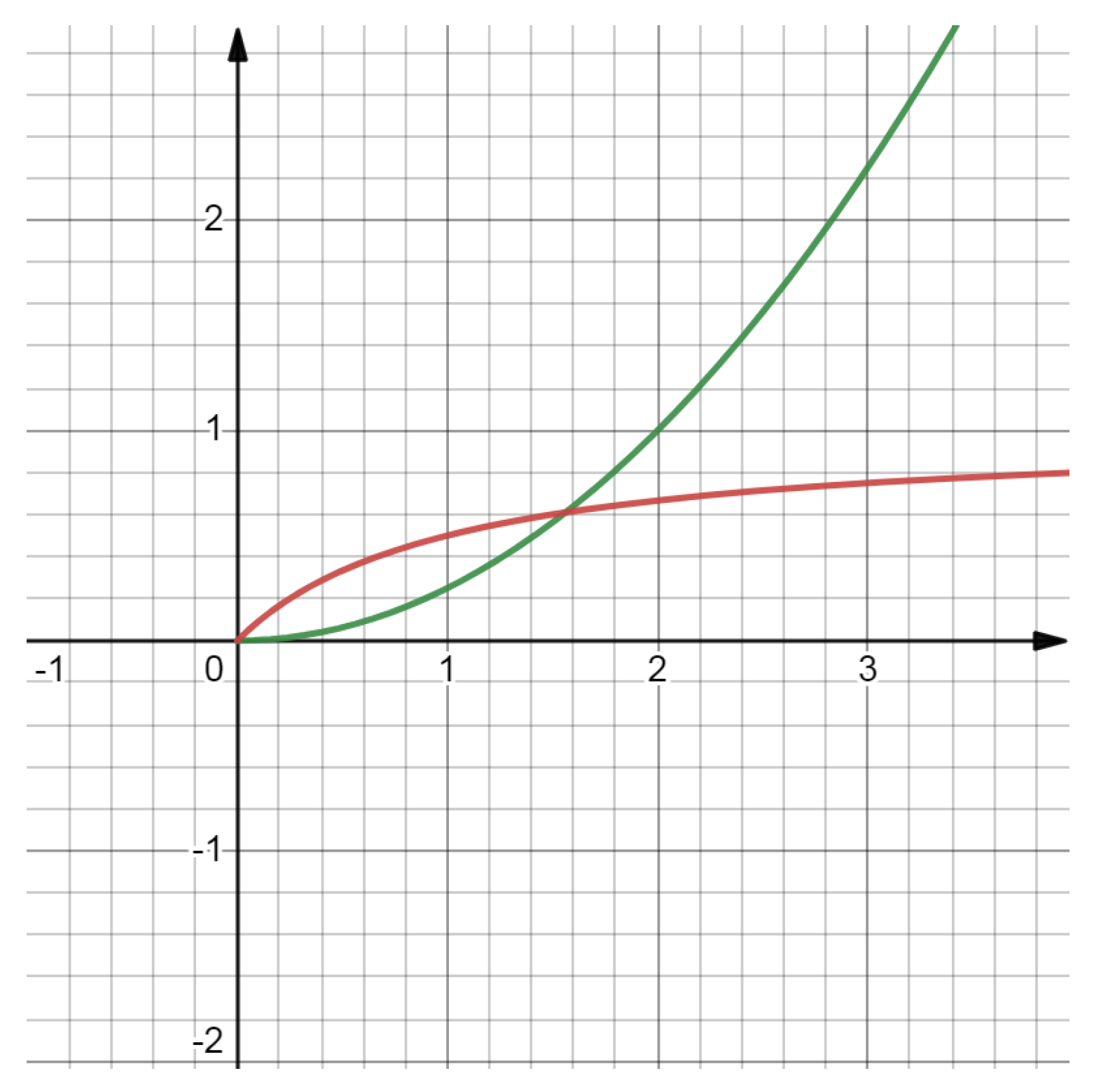
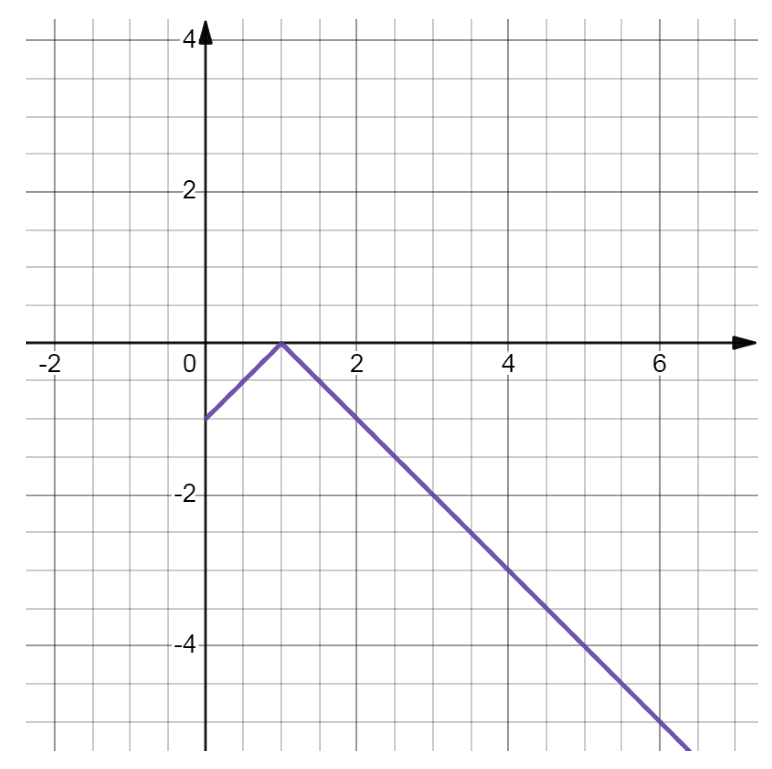
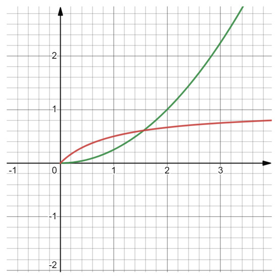
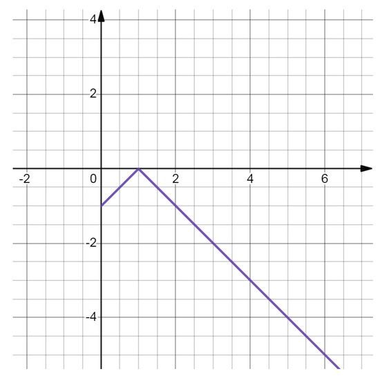
The above result is seen in the following Figure 1 and Figure 2. Therefore, $(\overline{x},\overline{\alpha },\overline{\mu },\overline{\nu })$ is a quasi ε-weak saddle point of the problem (NRMFP).

Figure 1. The illustration of $\mathcal{L}(x,\overline{\alpha },\overline{\mu },\overline{\nu })+\epsilon \parallel x-\overline{x}\parallel -\mathcal{L}(\overline{x},\overline{\alpha },\overline{\mu },\overline{\nu })$.

Figure 2. The illustration of $\mathcal{L}(\overline{x},\overline{\alpha },\mu ,\nu )-\epsilon \parallel \mu -\overline{\mu }\parallel$.

Theorem 3.

In the problem (NRMFP), suppose that $\overline{x}\in \mathcal{F}$ is a quasi-weak ε-efficient solution of the problem (NRMFP) and Theorem 1 is satisfied. If $(f,h,g)$ is an approximate convex function at $\overline{x}$, then $(\overline{x},\overline{\alpha },\overline{\mu },\overline{\nu })\in \mathcal{F}\times ({\mathbb{R}}_{+}^l\backslash \{0\})\times {\mathbb{R}}_{+}^n\times gphV$ is a quasi $\overline{\alpha }\epsilon$-weak saddle point, where $\overline{\alpha }\epsilon =({\overline{\alpha }}_1{\epsilon }_1,\cdots {\overline{\alpha }}_l{\epsilon }_l)$.

Proof. 

Firstly, we verify (10) holds. Since $\overline{x}$ is a quasi-weak $\epsilon$-efficient solution of the NRMFP, it follows from Theorem 1 that

$$\begin{array}{c}\hfill 0\in \sum _{i=1}^l{\overline{\lambda }}_i(\partial f_i(\overline{x})-\frac{f_i(\overline{x})}{h_i(\overline{x})}\partial h_i(\overline{x}))+\sum _{j=1}^n{\overline{\mu }}_j{\partial }_x{g}_{{\overline{t}}_j}(\overline{x},{\overline{v}}_j)+\sum _{i=1}^l{\overline{\alpha }}_i{\epsilon }_i\mathbb{B},\end{array}$$

$${\overline{\mu }}_j{g}_{{\overline{t}}_j}(\overline{x},{\overline{v}}_j)=0,\forall j=1,\cdots ,n.$$

Therefore, there exist ${\overline{\xi }}_i\in \partial f_i(\overline{x})$, ${\overline{\eta }}_i\in \partial h_i(\overline{x})$, ${\overline{\delta }}_j\in {\partial }_x{g}_{{\overline{t}}_j}(\overline{x},{\overline{v}}_j)$, and ${\overline{b}}_i\in \mathbb{B}$ such that

$$0=\sum _{i=1}^l{\overline{\lambda }}_i({\overline{\xi }}_i-\frac{f_i(\overline{x})}{h_i(\overline{x})}{\overline{\eta }}_i)+\sum _{j=1}^n{\overline{\mu }}_j{\overline{\delta }}_j+\sum _{i=1}^l{\overline{\alpha }}_i{\epsilon }_i{\overline{b}}_i.$$

Due to ${\overline{b}}_i\in \mathbb{B}$, for $x\in \mathcal{F}$, $⟨{\overline{b}}_i,x-\overline{x}⟩\le \parallel x-\overline{x}\parallel$, we have

$$⟨\sum _{i=1}^l{\overline{\lambda }}_i({\overline{\xi }}_i-\frac{f_i(\overline{x})}{h_i(\overline{x})}{\overline{\eta }}_i)+\sum _{j=1}^n{\overline{\mu }}_j{\overline{\delta }}_j,x-\overline{x}⟩+\sum _{i=1}^l{\overline{\alpha }}_i{\epsilon }_i\parallel x-\overline{x}\parallel \ge 0.$$

(12)

Suppose that $(\overline{x},\overline{\alpha },\overline{\mu },\overline{\nu })$ is not a quasi $\epsilon$-weak saddle point of the problem (NRMFP); then, there exists $\widehat{x}\in \mathcal{F}$ such that

$$\mathcal{L}(\widehat{x},\overline{\alpha },\overline{\mu },\overline{\nu })+\overline{\alpha }\epsilon \parallel \widehat{x}-\overline{x}\parallel -\mathcal{L}(\overline{x},\overline{\alpha },\overline{\mu },\overline{\nu })\in -{\mathbb{R}}_{++}^l.$$

From (9), we deduce

$$\overline{\alpha }(\frac{f(\widehat{x})}{h(\widehat{x})}-\frac{f(\overline{x})}{h(\overline{x})})+\frac{1}{l}\sum _{j=1}^n{\overline{\mu }}_j(g_{{\overline{t}}_j}(\widehat{x},{\overline{v}}_j)-g_{{\overline{t}}_j}(\overline{x},{\overline{v}}_j))e+\overline{\alpha }\epsilon \parallel \widehat{x}-\overline{x}\parallel \in -{\mathbb{R}}_{++}^l.$$

Thus,

$${\overline{\alpha }}_i(\frac{f_i(\widehat{x})}{h_i(\widehat{x})}-\frac{f_i(\overline{x})}{h_i(\overline{x})})+\frac{1}{l}\sum _{j=1}^n{\overline{\mu }}_j(g_{{\overline{t}}_j}(\widehat{x},{\overline{v}}_j)-g_{{\overline{t}}_j}(\overline{x},{\overline{v}}_j))+{\overline{\alpha }}_i{\epsilon }_i\parallel \widehat{x}-\overline{x}\parallel <0,i=1,\cdots ,l.$$

(13)

Since $(f,h,g)$ is an approximate convex function at $\overline{x}$, there exist $\overline{{\xi }_i}\in \partial f_i(\overline{x})$, ${\overline{\eta }}_i\in \partial h_i(\overline{x})$ and ${\overline{\delta }}_j\in {\partial }_x{g}_{{\overline{t}}_j}(\overline{x},{\overline{v}}_j)$ such that

$$\frac{f_i(\widehat{x})}{h_i(\widehat{x})}-\frac{f_i(\overline{x})}{h_i(\overline{x})}\ge \frac{1}{h_i(\overline{x})}(⟨\overline{{\xi }_i},\widehat{x}-\overline{x}⟩-\frac{f_i(\overline{x})}{h_i(\overline{x})}⟨{\overline{\eta }}_i,\widehat{x}-\overline{x}⟩),i=1,\cdots ,l,$$

$$g_{{\overline{t}}_j}(\widehat{x},{\overline{v}}_j)-g_{{\overline{t}}_j}(\overline{x},{\overline{v}}_j)\ge ⟨{\overline{\delta }}_j,\widehat{x}-\overline{x}⟩,j=1,\cdots ,n.$$

Let $\frac{{\overline{\alpha }}_i}{h_i(\overline{x})}={\overline{\lambda }}_i,i=1,\cdots ,l$, and then together with (13) we have

$${\overline{\lambda }}_i⟨({\overline{\xi }}_i-\frac{f_i(\overline{x})}{h_i(\overline{x})}{\overline{\eta }}_i),\widehat{x}-\overline{x}⟩+\frac{1}{l}⟨\sum _{j=1}^n{\overline{\mu }}_j{\overline{\delta }}_j,\widehat{x}-\overline{x}⟩+{\overline{\alpha }}_i{\epsilon }_i\parallel \widehat{x}-\overline{x}\parallel <0,i=1,\cdots ,l.$$

Then, we obtain

$$⟨\sum _{i=1}^l{\overline{\lambda }}_i({\overline{\xi }}_i-\frac{f_i(\overline{x})}{h_i(\overline{x})}{\overline{\eta }}_i),\widehat{x}-\overline{x}⟩+⟨\sum _{j=1}^n{\overline{\mu }}_j{\overline{\delta }}_j,\widehat{x}-\overline{x}⟩+\sum _{i=1}^l{\overline{\alpha }}_i{\epsilon }_i\parallel \widehat{x}-\overline{x}\parallel <0,$$

which contradicts (12).

Next, we prove (11) holds. Since ${\overline{\mu }}_j{g}_{{\overline{t}}_j}(\overline{x},{\overline{v}}_j)=0$, for any ${\mu }_j\ge 0,(t_j,v_j)\in (gphV),i=1,\cdots ,l$, we have ${\mu }_j{g}_{t_j}(\overline{x},v_j)\le 0$; hence,

$$\begin{array}{c}\hfill \sum _{j=1}^n{\overline{\mu }}_j{g}_{{\overline{t}}_j}(\overline{x},{\overline{v}}_j)-\sum _{j=1}^n{\mu }_j{g}_{t_j}(\overline{x},v_j)\ge 0.\end{array}$$

That is,

$$\begin{array}{ccc}& & -\overline{\alpha }\epsilon \parallel {\mu }_j-{\overline{\mu }}_j\parallel \leqq (0,\cdots ,0)\leqq \overline{\alpha }(\frac{f(\overline{x})}{h(\overline{x})}-\frac{f(\overline{x})}{h(\overline{x})})+\hfill \\ & & \frac{1}{l}\sum _{j=1}^n{\overline{\mu }}_j{g}_{{\overline{t}}_j}(\overline{x},{\overline{v}}_j)e-\overline{\alpha }(\frac{f(\overline{x})}{h(\overline{x})}-\frac{f(\overline{x})}{h(\overline{x})})-\frac{1}{l}\sum _{j=1}^n{\mu }_j{g}_{t_j}(\overline{x},v_j)e,\hfill \end{array}$$

which implies that

$$\mathcal{L}(\overline{x},\overline{\alpha },\mu ,\nu )-\overline{\alpha }\epsilon \parallel {\mu }_j-{\overline{\mu }}_j\parallel \leqq \mathcal{L}(\overline{x},\overline{\alpha },\overline{\mu },\overline{\nu }).$$

The next Theorem 4 shows that a quasi $\overline{\alpha }\epsilon$-weak saddle point is a quasi-weak $\epsilon$-efficient solution of the problem (NRMFP). □

Theorem 4.

In the problem (NRMFP), if $(\overline{x},\overline{\alpha },\overline{\mu },\overline{\nu })\in \mathcal{F}\times {\mathbb{R}}_{++}^l\times {\mathbb{R}}_{+}^n\times gphV$ is a quasi $\overline{\alpha }\epsilon$-weak saddle point and $\overline{x}$ is an optimal solution of the problem $max{\sum }_{j=1}^n{\overline{\mu }}_j{g}_{{\overline{t}}_j}(x,{\overline{v}}_j)$, then $\overline{x}$ is a quasi-weak ε-efficient solution, where $\overline{\alpha }\epsilon =({\overline{\alpha }}_1{\epsilon }_1,\cdots {\overline{\alpha }}_l{\epsilon }_l)$.

Proof. 

Since $(\overline{x},\overline{\alpha },\overline{\mu },\overline{\nu })$ is a quasi $\overline{\alpha }\epsilon$-weak saddle point of the problem (NRMFP), it follows from (10) that

$$\begin{array}{ccc}& & \overline{\alpha }(\frac{f(x)}{h(x)}-\frac{f(\overline{x})}{h(\overline{x})})+\frac{1}{l}\sum _{j=1}^n{\overline{\mu }}_j{g}_{{\overline{t}}_j}(x,{\overline{v}}_j)e+\overline{\alpha }\epsilon \parallel x-\overline{x}\parallel \hfill \\ & & -\overline{\alpha }(\frac{f(\overline{x})}{h(\overline{x})}-\frac{f(\overline{x})}{h(\overline{x})})-\frac{1}{l}\sum _{j=1}^n{\overline{\mu }}_j{g}_{{\overline{t}}_j}(\overline{x},{\overline{v}}_j)e\notin -{\mathbb{R}}_{++}^l,\forall x\in \mathcal{F}.\hfill \end{array}$$

(14)

Because $\overline{x}$ is an optimal solution of the problem $max{\sum }_{j=1}^n{\overline{\mu }}_j{g}_{{\overline{t}}_j}(x,{\overline{v}}_j)$, it holds that

$$\sum _{j=1}^n{\overline{\mu }}_j{g}_{{\overline{t}}_j}(x,{\overline{v}}_j)-\sum _{j=1}^n{\overline{\mu }}_j{g}_{{\overline{t}}_j}(\overline{x},{\overline{v}}_j)\le 0,\forall x\in \mathcal{F}.$$

(15)

Together with (14) and (15), we obtain

$$\overline{\alpha }(\frac{f(x)}{h(x)}-\frac{f(\overline{x})}{h(\overline{x})})+\overline{\alpha }\epsilon \parallel x-\overline{x}\parallel \notin -{\mathbb{R}}_{++}^l,\forall x\in \mathcal{F}.$$

Note that $\overline{\alpha }\in {\mathbb{R}}_{++}^l$, and we obtain

$$(\frac{f(x)}{h(x)}-\frac{f(\overline{x})}{h(\overline{x})})+\epsilon \parallel x-\overline{x}\parallel \notin -{\mathbb{R}}_{++}^l,\forall x\in \mathcal{F}.$$

Hence, $\overline{x}$ is a quasi-weak $\epsilon$-efficient solution of the problem (NRMFP). □

5. Conclusions

We have established a necessary condition for robust approximate quasi-weak efficient solutions of a problem (NUMFP) based on the properties of the Gerstewitz’s function. We have also introduced two kinds of generalized convex function pairs for the problem (NUMFP), and under their assumptions we have presented sufficient conditions and saddle point theorems for robust approximate quasi-weak efficient solutions.

It would be meaningful to further investigate the proper efficient solutions, duality theorems and some special applications for the problem (NUMFP), such as multiobjective optimization problems and minimax optimization problems. Indeed, ref. [4] has discussed duality theorems and special applications for a nonsmooth semi-infinite multiobjective optimization problem, respectively. Therefore, the further works seem feasible.

References

- Khantree, C.; Wangkeeree, R. On quasi approximate solutions for nonsmooth robust semi-infinite optimization problems. Carpathian J. Math. 2019, 35, 417–426. [Google Scholar] [CrossRef]
- Kanzi, N.; Nobakhtian, S. Nonsmooth semi-infinite programming problems with mixed constraints. J. Math. Anal. Appl. 2009, 351, 170–181. [Google Scholar] [CrossRef]
- Sun, X.K.; Teo, K.L.; Zeng, J. Robust approximate optimal solutions for nonlinear semi-infinite programming with uncertainty. Optimization 2020, 69, 2109–2129. [Google Scholar] [CrossRef]
- Pham, T.H. On Isolated/Properly Efficient Solutions in Nonsmooth Robust Semi-infinite Multiobjective Optimization. Bull. Malays. Math. Sci. Soc. 2023, 46, 73. [Google Scholar] [CrossRef]
- Chuong, T.D. Nondifferentiable fractional semi-infinite multiobjective optimization problems. Oper. Res. 2016, 44, 260–266. [Google Scholar] [CrossRef]
- Mishra, S.K.; Jaiswal, M. Optimality and duality for nonsmooth multiobjective fractional semi-infinite programming problem. Adv. Nonlinear Var. Inequalities 2013, 16, 69–83. [Google Scholar]
- Antczak, T. Sufficient optimality conditions for semi-infinite multiobjective fractional programming under (Φ,ρ)-V-invexity and generalized (Φ,ρ)-V-invexity. Filomat 2017, 30, 3649–3665. [Google Scholar] [CrossRef]
- Pan, X.; Yu, G.L.; Gong, T.T. Optimality conditions for generalized convex nonsmooth uncertain multi-objective fractional programming. J. Oper. Res. Soc. 2022, 1, 1–18. [Google Scholar] [CrossRef]
- Dem’yanov, V.F.; Vasil’ev, L.V. Nondifferentiable Optimization. In Optimization Software; Inc. Publications Division: New York, NY, USA, 1985. [Google Scholar]
- Han, W.Y.; Yu, G.L.; Gong, T.T. Optimality conditions for a nonsmooth uncertain multiobjective programming problem. Complexity 2020, 2020, 1–8. [Google Scholar] [CrossRef]
- Long, X.J.; Huang, N.J.; Liu, Z.B. Optimality conditions, duality and saddle points for nondifferentiable multiobjective fractional programs. J. Ind. Manag. Optim. 2017, 4, 287–298. [Google Scholar] [CrossRef]
- Kuroiwa, D.; Lee, G.M. On robust multiobjective optimization. J. Nonlinear Convex. Anal. 2012, 40, 305–317. [Google Scholar]
- Ben-Tal, A.; Ghaoui, L.E.; Nemirovski, A. Robust Optimization; Princeton University Press: Princeton, NJ, USA, 2009; pp. 16–64. [Google Scholar]
- Caristi, G.; Ferrara, M. Necessary conditions for nonsmooth multiobjective semi-infinite problems using Michel-Penot subdifferential. Decis. Econ. Financ. 2017, 40, 103–113. [Google Scholar] [CrossRef]
- Kabgani, A.; Soleimani-damaneh, M. Characterization of (weakly/properly/robust) efficient solutions in nonsmooth semi-infinite multiobjective optimization using convexificators. Optimization 2018, 67, 217–235. [Google Scholar] [CrossRef]
- Clarke, F.H. Optimization and Nonsmooth Analysis; Wiley: New York, NY, USA, 1983; pp. 46–78. [Google Scholar]
- Fakhar, M.; Mahyarinia, M.R.; Zafarani, J. On nonsmooth robust multiobjective optimization under generalized convexity with applications to portfolio optimization. Eur. J. Oper. Res. 2018, 265, 39–48. [Google Scholar] [CrossRef]
- Lee, G.M.; Kim, G.S.; Dinh, N. Optimality Conditions for Approximate Solutions of Convex Semi-Infinite Vector Optimization Problems. Recent Dev. Vector Optim. 2012, 1, 275–295. [Google Scholar]
- Chen, J.W.; Köbis, E.; Yao, J.C. Optimality Conditions and Duality for Robust Nonsmooth Multiobjective Optimization Problems with Constraints. J. Optim. Theory Appl. 2019, 265, 411–436. [Google Scholar] [CrossRef]
- Gerth, C.; Weidner, P. Nonconvex separation theorems and some applications in vector optimization. J. Optim. Theory Appl. 1990, 67, 297–320. [Google Scholar] [CrossRef]
- Han, Y. Connectedness of the approximate solution sets for set optimization problems. Optimization 2022, 71, 4819–4834. [Google Scholar] [CrossRef]
- Rockafellar, R.T. Convex Analysis; Princeton University Press: Princeton, NJ, USA, 1997; pp. 10–32. [Google Scholar]
- Tung, N.M.; Van Duy, M. Constraint qualifications and optimality conditions for robust nonsmooth semi-infinite multiobjective optimization problems. 4OR 2022, 21, 151–176. [Google Scholar] [CrossRef]
Disclaimer/Publisher’s Note: The statements, opinions and data contained in all publications are solely those of the individual author(s) and contributor(s) and not of MDPI and/or the editor(s). MDPI and/or the editor(s) disclaim responsibility for any injury to people or property resulting from any ideas, methods, instructions or products referred to in the content. |
© 2023 by the authors. Licensee MDPI, Basel, Switzerland. This article is an open access article distributed under the terms and conditions of the Creative Commons Attribution (CC BY) license (https://creativecommons.org/licenses/by/4.0/).