General Exact Schemes for Second-Order Linear Differential Equations Using the Concept of Local Green Functions

Abstract

In this paper, we introduce a special system of linear equations with a symmetric, tridiagonal matrix, whose solution vector contains the values of the analytical solution of the original ordinary differential equation (ODE) in grid points. Further, we present the derivation of an exact scheme for an arbitrary mesh grid and prove that its application can completely avoid other errors in discretization and numerical methods. The presented method is constructed on the basis of special local green functions, whose special properties provide the possibility to invert the differential operator of the ODE. Thus, the newly obtained results provide a general, exact solution method for the second-order ODE, which is also effective for obtaining the arbitrary grid, Dirichlet, and/or Neumann boundary conditions. Both the results obtained and the short case study confirm that the use of the exact scheme is efficient and straightforward even for ODEs with discontinuity functions.

1. Introduction

Consider the linear second order inhomogeneous ordinary differential equation (ODE):

$$Lu\left(x\right)=-\frac{d}{dx}\left(\kappa \left(x\right)\frac{d}{dx}u\left(x\right)\right)+q\left(x\right)u\left(x\right)=f\left(x\right)(0<x<\ell )$$

(1)

where $\kappa \left(x\right)\ge {\kappa }_0>0$ is a positive, arbitrary function, $q\left(x\right)$ and $f\left(x\right)$ are continuous functions and the function $u\left(x\right)$ is the solution of ODE on the finite closed interval $[0,\ell ]$.

The use of boundary value problem (BVP) with Equation (1) for modeling physical phenomena is very rare in the relevant literature. A large part of the possible implicit application areas are the initial value problems (IVPs) prescribed by Equation (1) with constant coefficients. BVPs including the coefficients of the resistance (R), capacity (C) and inductance (L) can be used to model RLC circuits [1]. It is also well known that the IVP for Equation (1) is also used in harmonic analysis, where the coefficients are the spring constant, damping and mass [2]. Another group of applications consist of reaction diffusion equations, which, however, even in the simplest case, contain some nonlinear terms [3]. The third major field of science where equations such as Equation (1) can be found is the Sturm–Liouville theory [4]. In this case, although BVPs are solved for non-constant coefficient ODEs, equations can be interpreted as eigenvalue problems, and solutions are also known in special cases [4]. It follows that the BVPs defined by Equation (1) are a special group of ODEs. Perhaps the most well-known of these is the so-called Cauchy–Euler equation [5], where $\kappa \left(x\right)=x$, $q\left(x\right)=1/x$ and $f\left(x\right)=0$.

Although the solutions of the mathematical problems mentioned above are well known, since several mathematical methods have been developed for their production, solutions for non-constant coefficient equations are known only in special cases (for example, the Cauchy–Euler equation [5]). Common methods for solving non-constant coefficient IVPs are the constant variation method, the method of undetermined coefficients, etc. [5].

The BVPs with Equation (1) are usually solved using well-known numerical methods, such as the finite difference method (FDM) [6], the finite volume method (FVM) [7] and the boundary element method (BEM) [8], by approximating the analytical solution of the ODE. Among the classical numerical methods for solving second-order differential equations, the finite element method (FEM) is presently the most widely used [9]. Nothing better illustrates the challenges of BVP defined by Equation (1) than the fact that, even in recent years, we can find publications where the authors researched methods for solving the non-constant coefficient problem [10,11,12].

This research is motivated by two main research directions. One of these directions is the study of symbolic approaches related to non-linear ODEs and systems, the so-called reaction–diffusion, cross-diffusion equations [13,14]. Further, the research group is ambitious in studying other types of non-linear ODEs, which are still intensively researched today [15,16,17]. The second research area is the inverse problems involving second-order differential equations, which are also non-linear mathematical problems [18]. Still, compared to the classical differential equation solvers, they require a completely different handling, since the functions to be determined are the coefficients of the differential equation [19,20,21]. All these research activities are supported by a solid foundation in exact schemes, which, as effective and robust mathematical methods, provide new perspectives for basic research.

Finding and then applying an analytical solution to solve the physical problems minimizes the additional errors induced by mathematical techniques. These efforts have already motivated many researchers who, as a result of their work, have presented some higher-order schemes for first- and second-order differential equations, as were presented in [22]. Other authors have published papers about using the beneficial properties of the Bessel equation [5] to solve homogenous equations with a second-order ODE in order to obtain the analytic solution [23]. In the case of singular secondary ODEs, solvability is still the subject of mathematical studies. Kiguradze et al. [24,25,26] published several related studies that thoroughly examine the difficulties of these mathematical problems to be solved.

This research also aims to develop a new analytical solving techniques to solve the BVPs in case of Equation (1). During our research work, we developed an exact solution technique that uses the inverse of the differential operator to solve the ODE. The methods we have deployed propose schemes that provide the values for the exact solution (We define the exact solution as the value of the analytical solution at any given location.) of Equation (1) at arbitrarily chosen grid points. The specific properties of the exact schemes are the main novelty of the presented research, with the introduced strength of their application compared to other alternative methods. In fact, there are two possible implementations. In the first case, without a mesh, we can use them to define symbolically the analytical solution itself. In the second case, using a mesh, we produce the values of the analytical solution in terms of grid points, without needing to determine the analytical solution itself [27]. The main advantage of this characteristic is its robustness and efficiency, which makes it irrelevant for the method how many grid points are chosen inside the domain, since the calculated values will always be the values of the analytical solution in grid points [27]. Compared with alternative solution methods, the use of exact schemes also leads to the solution of a linear system of equations with outstanding properties, still the matrix and the right-hand side of the system of equations are constructed with special functions, and the integration leads to the stability required to solve the linear system of equations. All these beneficial properties are guaranteed by the so-called local green functions, whose concept was presented by Vizvari et al. [27]. Local Green functions differ from global green functions in the following. While global green functions can be used to symbolically represent the analytical solution of the ODE, on the other hand, the local green functions are defined on the mesh intervals with the same properties as global green functions and they are used to form the system of linear equations that are generated with the exact scheme.

The application concept of the local Green functions [27] opens the possibility to develop a mathematical method deriving a recursive formula which allows us to compute the values of the analytic solution in grid points using simple linear algebraic methods. In the self-adjoint case, when $q\left(x\right)=0$ for Equation (1), it has already been shown that integral functions of $\frac{1}{\kappa \left(x\right)}$ can be used to derive exact schemes using the apparatus of the FEM [27]. Using the electrical analogy, these local Green functions are integral functions of the material’s resistance, more precisely the resultant resistance of the material under investigation. In this paper, we also intend to use strictly positive test functions that generate the exact schemes based on the FEM apparatus for Equation (1) [9]. However, compared to the FEM, local green functions have the ability to invert the differential operator of the ODE as a result of performing the necessary partial integration. Based on the previous results [27], the local green functions have the same properties as the integrals of $\frac{1}{\kappa \left(x\right)}$; however, in this case, the local green functions are the results of solving a special initial value problem, since this guarantees the existence of the necessary and important properties that the exact scheme exploits. These facts complicate the results published in the previous work [27], since the solution of the initial value problem for a homogeneous equation can only be solved by using symbolic techniques, since here the goal is to generate functions. After all, the implementation of the exact scheme is possible even by fully numerical methods, since the use of local green functions and the necessary mathematical manipulations lead to discrete values of the analytical solution. The robustness and efficiency of the application of local green functions and exact schemes are best demonstrated by the solvability of ODEs with discontinuity functions and/or singular points, which will be presented in detail in the case studies.

Thus, the research of exact schemes is an important aspect in the domain of mathematical physics, and increasing the accuracy of such schemes is a continuous challenge for researchers. Furthermore, increasing the accuracy also increases the complexity and computational burden of the schemes, resulting in difficulties in applicability. However, our proposed schemes can overcome these limitations, as they provide the exact solution at an arbitrary location independent from the space discretization. Based on this fact, our research team have developed exact schemes for the symmetric, self-adjoint case ($q\left(x\right)=0$), that also work robustly for Dirichlet and mixed boundary conditions [27]. In this paper, as a continuation of our research work [27] and as a generalization of the self-adjoint case ($q\left(x\right)\ne$0), we present our latest results in the field of exact schema research work. In the following sections, we will introduce the application of the exact scheme to Equation (1).

This paper is structured as follows. The first section is the introduction, and the second section presents the exact schemes developed for two cases. The first subsection introduces the concept of local green functions, the second subsection defines the exact scheme with the Dirichlet boundary condition [5] prescribed in both endpoints, and the third subsection shows the handling of mixed boundary conditions, where Dirichlet at one and Neumann boundary condition [5] at the other endpoint are prescribed. The third section introduces a brief case study with discontinuous function $\kappa \left(x\right)$. From these results, the fourth section draws the conclusions and establishes the future work.

2. The Exact Schemes

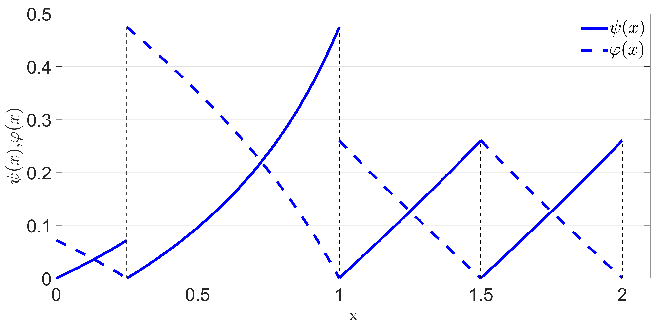
2.1. The Concept of Local Green Functions

As a first step in the concept of local green functions and by obtaining the solution of the initial value problems in Equations (3) and (4), we define ($2n$) non-negative functions on different subintervals. The exact scheme is generated based on a special symmetric system of the local Green functions. Now, let us consider an arbitrary discretization of the interval $[0,\ell ]$ into $(n+1)$ subintervals:

$$x_0=0<x_1<\cdots <x_{i-1}<x_i<x_{i+1}<\cdots <x_{n-1}<x_n<x_{n+1}=\ell$$

(2)

where $x_i$ is the $i^{th}$ grid point in interval $[0,\ell ]$ ($i=0\cdots n+1$). Using these discretization, the local green functions are defined as the solutions of the initial value problems described in Equations (3) and (4):

$$\{\begin{array}{}\text{(3a)}& L{\psi }_{i-1}\left(x\right)=0\hfill \text{(3b)}& {\psi }_{i-1}\left(x_{i-1}\right)=0\hfill \text{(3c)}& \kappa \left(x_{i-1}\right)\frac{d}{dx}{\psi }_{i-1}\left(x_{i-1}\right)=1\hfill \end{array}$$

on interval $x\in I_{i-1}=[x_{i-1},x_i]$ and

$$\{\begin{array}{}\text{(4a)}& L{\phi }_i\left(x\right)=0\hfill \text{(4b)}& {\phi }_i\left(x_{i+1}\right)=0\hfill \text{(4c)}& \kappa \left(x_{i+1}\right)\frac{d}{dx}{\phi }_i\left(x_{i+1}\right)=-1\hfill \end{array}$$

on interval $x\in I_i=[x_i,x_{i+1}]$, where $i=1,2,\cdots ,n$. Based on this, in order to produce the exact scheme, we need a positive monotonically increasing function (${\psi }_{i-1}\left(x\right)$) and a positive, but monotonically decreasing function (${\phi }_i\left(x\right)$), which we have defined as a solution to the initial value problem corresponding to a homogeneous equation and the appropriate initial conditions. From the derivatives listed in Equations (3) and (4), it is clear that the test functions ${\psi }_i$ increase monotonically and ${\phi }_i$ decreases symmetrically on the interval of their domain $[x_i,x_{i+1}]$ for all $i=1,2,\cdots ,n-1$. On the first interval $[x_0,x_1]$, only the test function ${\psi }_0$ is considered; and on the last interval $[x_n,x_{n+1}]$, we define only the test function ${\phi }_n$ similar to the function in the FEM [9]. Based on the equalities in (3) and (4), these test functions can be considered as local green functions [27], which have the following useful property:

Theorem 1

(Symmetry of local green functions). Consider the $[x_i,x_{i+1}]$ subinterval of the partition (2) of interval $[0,\ell ]$. Let ${\psi }_i\left(x\right)$ and ${\phi }_i\left(x\right)$ be the test functions defined on subinterval $[x_i,x_{i+1}]$ based on (3) and (4). The test functions ${\psi }_i\left(x\right)$ and ${\phi }_i\left(x\right)$ are equal at the appropriate endpoints of the $[x_i,x_{i+1}]$ interval, i.e.,:

$${\psi }_i\left(x_{i+1}\right)={\phi }_i\left(x_i\right)=:\frac{1}{a_i}$$

(5)

where $i=1,2,\cdots ,(n-1)$ and $a_i$ is the $i^{th}$ coefficient of the constructed system of linear equations.

Proof 

To prove the Theorem 1, in the first step, multiply Equation (1) by ${\psi }_i\left(x\right)$ and in the second step by ${\phi }_i\left(x\right)$, subtract them from each other and integrate the difference on interval $[x_i,x_{i+1}]$ with respect to x (using the properties presented in the Equations (3a) and (4a)):

$$\begin{array}{cc}\hfill 0& ={\int }_{x_i}^{x_{i+1}}\left({\psi }_i\left(x\right)L{\phi }_i\left(x\right)-{\phi }_i\left(x\right)L{\psi }_i\left(x\right)\right)dx\hfill \\ \hfill & =-{\int }_{x_i}^{x_{i+1}}{\psi }_i\left(x\right){\left(\kappa \left(x\right){\phi }_i^{\prime }\left(x\right)\right)}^{\prime }dx+{\int }_{x_i}^{x_{i+1}}{\psi }_i\left(x\right)q\left(x\right){\phi }_i\left(x\right)dx\hfill \\ \hfill & +{\int }_{x_i}^{x_{i+1}}{\phi }_i\left(x\right){\left(\kappa \left(x\right){\psi }_i^{\prime }\left(x\right)\right)}^{\prime }dx-{\int }_{x_i}^{x_{i+1}}{\phi }_i\left(x\right)q\left(x\right){\psi }_i\left(x\right)dx\hfill \end{array}$$

(6)

where the prime (${}^{\prime }$) denotes the derivative with respect to x. After simplification and applying integration by parts on the right-hand side, the following form is obtained:

$$\begin{array}{cc}\hfill 0& =-{\psi }_i\left(x_{i+1}\right)\kappa \left(x_{i+1}\right){\phi }_i^{\prime }\left(x_{i+1}\right)+{\psi }_i\left(x_i\right)\kappa \left(x_i\right){\phi }_i^{\prime }\left(x_i\right)\hfill \\ \hfill & +{\phi }_i\left(x_{i+1}\right)\kappa \left(x_{i+1}\right){\psi }_i^{\prime }\left(x_{i+1}\right)-{\phi }_i\left(x_i\right)\kappa \left(x_i\right){\psi }_i^{\prime }\left(x_i\right)\hfill \end{array}$$

(7)

Taking advantage of the special properties of the test functions (Equations (3b), (4b), (3c) and (4c)), the formula is simplified to:

$$0={\psi }_i\left(x_{i+1}\right)-{\phi }_i\left(x_i\right)(i=1,2,\cdots ,n)$$

(8)

This proves Theorem 1. □

Having introduced the symmetric concept of local green functions, the properties presented in Equations (3) and (4) and Theorem 1 allow us to construct the exact schemes as follows.

2.2. Dirichlet Boundaries

In the case of Dirichlet boundaries [5], the values of the solution at the endpoints are obtained as follows:

$${\mathfrak{B}}_D=\left\{u\left(0\right)=\alpha ,u(\ell )=\beta \right\}$$

(9)

where ${\mathfrak{B}}_D$ is the set of Dirichlet boundary conditions [5].

The scheme that is used to obtain exact solutions to the Dirichlet problem in Equation (1) is described by the following theorem:

Theorem 2

(Exact Dirichlet scheme). If ${\psi }_{i-1}\left(x\right)$ and ${\phi }_i\left(x\right)$ are the test functions [9] satisfying the Equation (3), the Equation (4), respectively, and Theorem 1, the solution vector from following the exact scheme yields to the values of the analytical solution of Equation (1) at the grid points with boundary conditions in Equation (9). Equations (3) and (4) are special IVPs defined based on the homogeneous equation corresponding to the original ODE (Equation (1)).

Let us consider a system of $n\ge 3$ linear equations:

$$\left\{\begin{array}{cc}{b}_1{u}_1-a_1{u}_2& =a_0\alpha +a_0{G}_0+a_1{H}_1\hfill \\ -a_{i-1}{u}_{i-1}+b_i{u}_i-a_i{u}_{i+1}& =a_{i-1}{G}_{i-1}+a_i{H}_i\hfill \\ -a_{n-1}{u}_{n-1}+b_n{u}_n& =a_n\beta +a_{n-1}{G}_{n-1}+a_n{H}_n\hfill \end{array}\right.$$

(10)

with indexes $i=2,3,\cdots ,(n-1)$. The solution vector of Equation (10) $U={(u_1,u_2,\cdots ,u_n)}^T$ leads to the same values as the solution $u\left(x\right)$ of the second-order ODE (1) with boundary conditions (9) at the interior grid points (2) without any error; that is, $u\left(x_i\right)=u_i$. The matrix of the system of linear equations constructed by recursion (Equation (10)) is a tridiagonal, symmetric, diagonally dominant (if $q\left(x\right)\ne 0$), $n\times n$ matrix, whose inverse exists in all cases.

The coefficients in Equation (10) are defined as

$$a_{i-1}=\frac{1}{{\psi }_{i-1}\left(x_i\right)}=\frac{1}{{\phi }_i\left(x_{i-1}\right)}$$

(11)

$$b_i=a_{i-1}\left(1+{\int }_{x_{i-1}}^{x_i}q\left(x\right){\psi }_{i-1}\left(x\right)dx\right)+a_i\left(1+{\int }_{x_i}^{x_{i+1}}q\left(x\right){\phi }_i\left(x\right)dx\right)$$

(12)

$$G_{i-1}={\int }_{x_{i-1}}^{x_i}f\left(t\right){\psi }_{i-1}\left(t\right)dt$$

(13)

$$H_i={\int }_{x_i}^{x_{i+1}}f\left(t\right){\phi }_i\left(t\right)dt$$

(14)

where $i=1,2,\cdots ,n$.

Proof 

In the first step, we multiply the ODE (1) by ${\psi }_{i-1}\left(x\right)$ and integrate it over $I_{i-1}$:

$${\int }_{x_{i-1}}^{x_i}Lu\left(x\right){\psi }_{i-1}\left(x\right)dx={\int }_{x_{i-1}}^{x_i}f\left(x\right){\psi }_{i-1}\left(x\right)dx=G_{i-1}.$$

(15)

After applying partial integration, the following expression is derived using the properties of ${\psi }_{i-1}$ and multiplying with $a_{i-1}$ (based on Equation (3)):

$$-\kappa \left(x_i\right)u^{\prime }\left(x_i\right)+a_{i-1}(u\left(x_i\right)\kappa \left(x_i\right){\psi }_{i-1}^{\prime }\left(x_i\right)-u\left(x_{i-1}\right))=a_{i-1}{G}_{i-1}.$$

(16)

Similarly, we multiply ODE (1) by ${\phi }_i\left(x\right)$ and integrate it over $I_i$ to obtain

$${\int }_{x_i}^{x_{i+1}}Lu\left(x\right){\phi }_i\left(x\right)dx={\int }_{x_i}^{x_{i+1}}f\left(x\right){\phi }_i\left(x\right)dx=H_i.$$

(17)

By applying partial integration, the following relation is obtained using the properties of ${\phi }_i$ and multiplying with $a_i$ (based on Equation (4)):

$$\kappa \left(x_i\right)u^{\prime }\left(x_i\right)-a_i(u\left(x_{i+1}\right)+u\left(x_i\right)\kappa \left(x_i\right){\phi }_i^{\prime }\left(x_i\right))=a_i·H_i.$$

(18)

The fundamental recursive formula is obtained by adding Equation (16) and Equation (18), and using the equalities

$$\kappa \left(x_i\right){\psi }_{i-1}^{\prime }\left(x_i\right)=1+{\int }_{x_{i-1}}^{x_i}q\left(x\right){\psi }_{i-1}\left(x\right)dx$$

(19)

and

$$\kappa \left(x_i\right){\phi }_i^{\prime }\left(x_i\right)=-1-{\int }_{x_i}^{x_{i+1}}q\left(x\right){\phi }_i\left(x\right)dx$$

(20)

obtaining from $L{\psi }_{i-1}\left(x\right)=0$ and $L{\phi }_i\left(x\right)=0$, respectively, we obtain:

$$-a_{i-1}u\left(x_{i-1}\right)+b_{i}u\left(x_i\right)-a_{i}u\left(x_{i+1}\right)=a_{i-1}{G}_{i-1}+a_i{H}_i.$$

(21)

If we substitute $i=1,2,3,\cdots ,n$ and $u\left(0\right)=\alpha$, $u(\ell )=\beta$, we obtain Equation (10) in Theorem 2. It follows that:

$$u\left(x_i\right)=u_i(i=1,2,...,n)$$

(22)

where $u\left(x_i\right)$ is the value of the analytical solution of the Equation (1) in the $i^{th}$ mesh point and $u_i$ is the $i^{th}$ element of the solution vector U. □

2.3. Exact Scheme for Dirichlet and Neumann Boundaries

In this case, we obtain the solution of the ODE (Equation (1)) using the following boundary conditions:

$${\mathfrak{B}}_{DN}=\left\{u\left(0\right)=\alpha ,\kappa (\ell )u^{\prime }(\ell )=\delta \right\}.$$

(23)

Owing to the definition of the boundary conditions in Equation (23), the Dirichlet scheme cannot be used directly to obtain the values of the exact solution. However, the value of $u(\ell )$ can be calculated using $\beta$ by defining the Neumann-to-Dirichlet transformation. Consider that the same manipulations lead to the identity (16), albeit on the entire interval $[0,\ell ]$. In this case, we obtain:

$$\begin{array}{cc}\hfill & -\kappa (\ell )u^{\prime }(\ell )+\frac{1}{{\psi }_0(\ell )}\left[u(\ell )\left(1+{\int }_0^{\ell }q\left(x\right){\psi }_0\left(x\right)dx\right)-u\left(0\right)\right]=\frac{1}{{\psi }_0(\ell )}{\int }_0^{\ell }f\left(t\right){\psi }_0\left(t\right)dt.\hfill \end{array}$$

(24)

After the substitution $\kappa (\ell )u^{\prime }(\ell )=\delta$, $u\left(0\right)=\alpha$ and isolating $u(\ell )$ from Equation (24), the Neumann boundary condition $\kappa (\ell )u^{\prime }(\ell )=\delta$ is transformed into the Dirichlet boundary value $u(\ell )$, which can be substituted directly in the result presented in Theorem 2. The result of the isolation is

$${\displaystyle u(\ell )=\frac{{\displaystyle \alpha +{\psi }_0(\ell )\delta +{\int }_0^{\ell }f\left(t\right){\psi }_0\left(t\right)dt}}{{\displaystyle 1+{\int }_0^{\ell }q\left(x\right){\psi }_0\left(x\right)dx}}.}$$

(25)

3. Case Studies with Discontinuous $\mathit{\kappa }\left(\mathit{x}\right)$ and Singular ODE

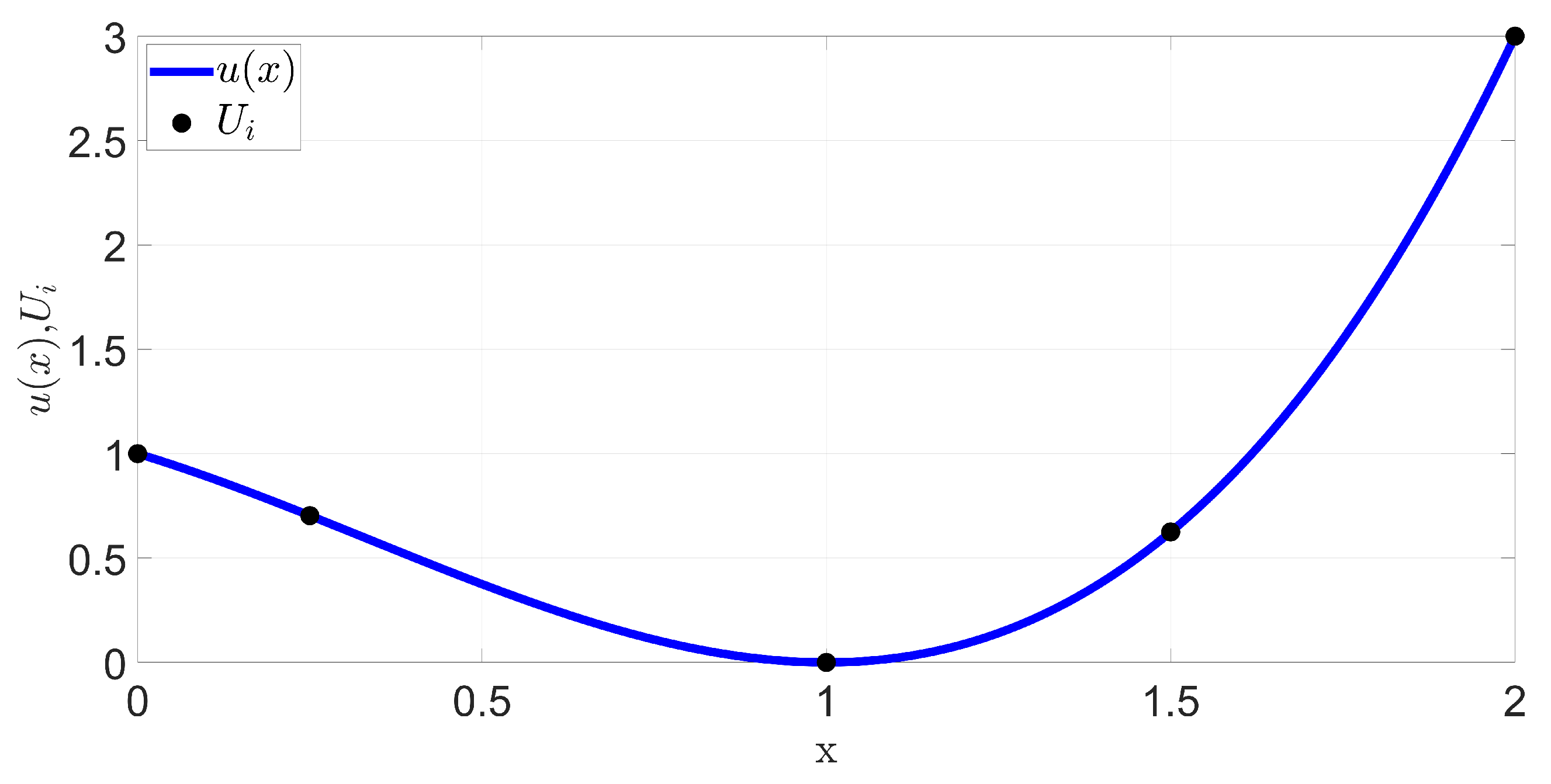
3.1. Implementation of the Exact Scheme to Solve Case Studies

In this section, we demonstrate the effectiveness and robustness of the proposed exact scheme in the case of a discontinuous $\kappa \left(x\right)$ and a regular singular ODE, that appear in several physical and mathematical problems based on Equation (1). However, before solving the case studies, consider generally the application of the exact scheme in a step-wise sequence:

1.

After defining the ODE to be solved and the necessary boundary conditions (Dirichlet problem, mixed problem), based on Equation (2), we perform an arbitrary partition of the interval $[0,\ell ]$. The indexes of the nodes are: $i=0,1,\cdots ,n-1,n,n+1$, where 0 and $n+1$ are the indices of the boundary points.

2.

Solving the initial value problems described with the Equations (3) and (4), we obtain the local Green functions ${\psi }_{i-1}\left(x\right)$ and ${\phi }_i\left(x\right)$, respectively ($i=1,2,\cdots ,n$).

3.

Based on Equations (11)–(14), we calculate all the coefficient values of the $a_{i-1}$, $b_i$, $G_{i-1}$ and $H_i$, respectively ($i=1,2,\cdots ,n$).

4.

Boundary conditions are also easily managed:

• For Dirichlet boundary conditions, we use the substitution defined in Equation (9),
• For mixed boundary conditions, we apply the Neumann to Dirichlet transformation based on the Equation (25) in order to calculate the potential value at the boundary point where the Neumann boundary condition is defined.

5.

Construct the linear system of equations defined in Equation (10), using the coefficient values and boundary conditions calculated before, and solve it by inverting the tridiagonal matrix.

6.

The elements of the vector obtained in this way are equal to the values of the analytic solution of the ODE defined in the first step taken in the grid points, according to the boundary conditions (according to Theorem 2).

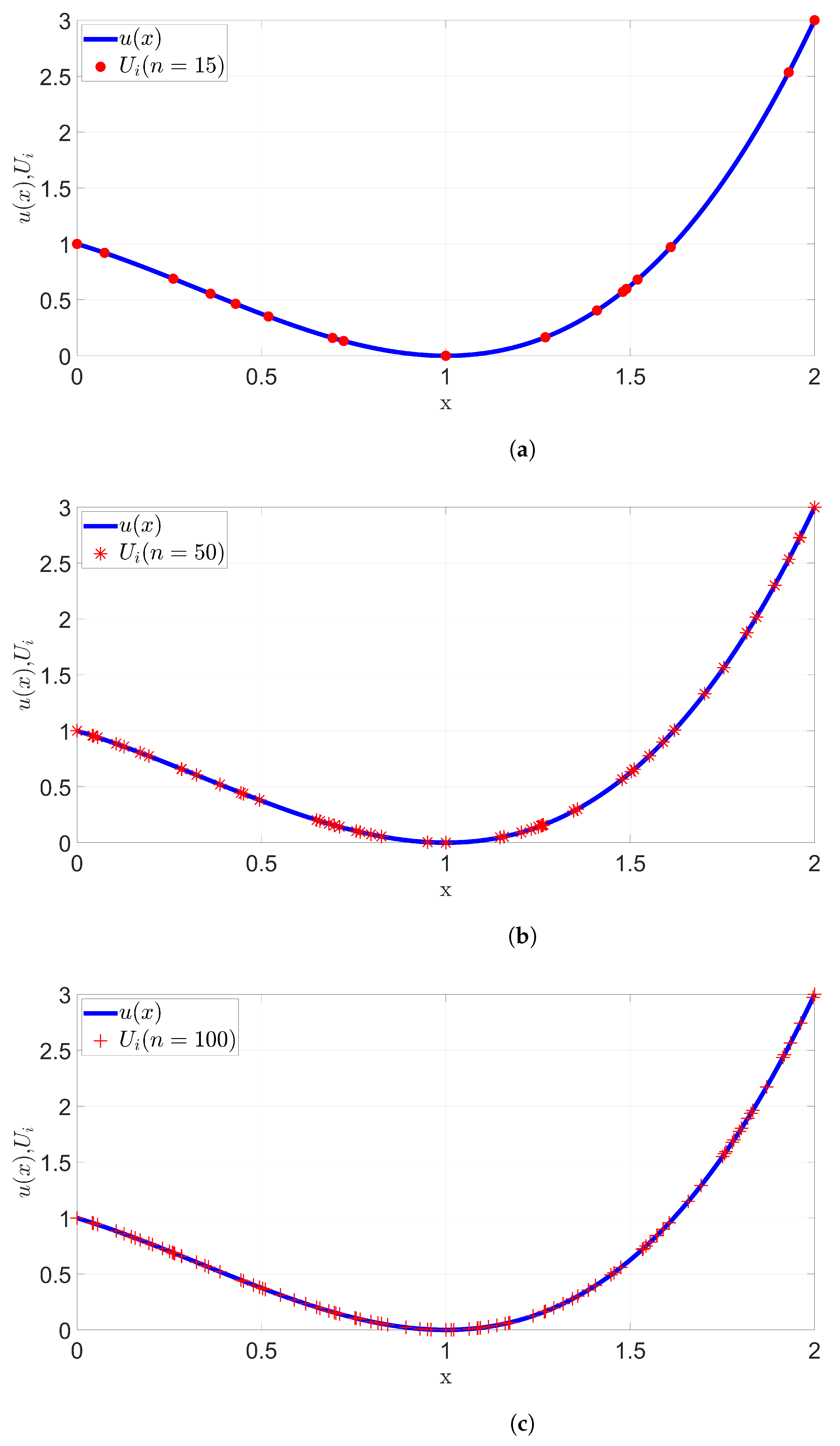
The case studies presented in this work have been evaluated symbolically and numerically using the MAPLE software package in order to be able to show the local green functions in a symbolic way.

3.2. A Case Study for Discontinuous $\kappa \left(x\right)$ with Increasing Mesh Resolution

First, we solve a Dirichlet and then a Dirichlet–Neumann problem using a mesh grid, wherein one of the grid points is provided at the breakpoint of the $\kappa \left(x\right)$ function. Let the functions in Equation (1) be a $q\left(x\right)=2$ constant,

$$\kappa \left(x\right)=\left\{\begin{array}{cc}{(x-2)}^2\hfill & \mathrm{if}x\le 1\hfill \\ 2\hfill & \mathrm{if}1<x\hfill \end{array}\right.$$

(26)

and

$$f\left(x\right)=\left\{\begin{array}{cc}-10x^3+40x^2-40x+6\hfill & \mathrm{if}x\le 1\hfill \\ 2x^3-2x^2-14x+6\hfill & \mathrm{if}1<x\hfill \end{array}\right.$$

(27)

discontinuous functions. The solution of a problem prescribed in this manner is

$$u\left(x\right)={(x-1)}^2(x+1)$$

(28)

on the interval $x\in [0,2]$ with

$${\mathfrak{B}}_{DN}=\left\{u\left(0\right)=1,u\left(2\right)=3\right\}$$

(29)

boundary conditions.

In this case study, our goal is to show the efficiency and robustness of the exact scheme by solving an ODE with $\kappa \left(x\right)$, $f\left(x\right)$ (presented in the Equations (26) and (27)) and constant $q\left(x\right)$ functions for several mesh partitions with increasing resolution. Consider the mesh point coordinates in the interval $[0,2]$ as follows:

$$\mathbf{x}=[0,\frac{1}{4},1,\frac{3}{2},2]$$

(30)

The values of $u\left(x\right)$ are determined using Theorem 2 in the grid points of the mesh. For the partitioning described in Equation (30), we divide the domain into 4 subintervals, i.e., $n+1=4$, hence we define the values of the analytic solution at $n=3$ points. The point of interest is $x_2=1$, which is exactly the breakpoint of $\kappa \left(x\right)$, where the analytic solution can also be determined using the exact scheme.

Consider first the mesh in Equation (30), which is defined based on instructions in Section 3.1 (point 1). According to point 2 in Section 3.1, Equations (3) and (4), the obtained local Green functions are defined in the Equation (31).

$${\psi }_0=\frac{1}{12}\frac{x\left(x^2-6x+12\right)}{{\left(-2+x\right)}^2}$$

(31a)

$${\psi }_1=\frac{1}{588}\frac{\left(4x-1\right)\left(16x^2-92x+169\right)}{{\left(-2+x\right)}^2}$$

(31b)

$${\psi }_2=\frac{1}{4}\left(e^{-1+x}-e^{1-x}\right)$$

(31c)

$${\psi }_3=-\frac{1}{4}\left(e^{-x+3/2}-e^{-3/2+x}\right)$$

(31d)

$${\phi }_1=-\frac{1}{588}\frac{\left(4x-1\right)\left(16x^2-92x+169\right)}{{\left(-2+x\right)}^2}$$

(31e)

$${\phi }_2=-\frac{1}{3}\frac{\left(-1+x\right)\left(x^2-5x+7\right)}{{\left(-2+x\right)}^2}$$

(31f)

$${\phi }_3=\frac{1}{4}\left({\mathrm{e}}^{-x+3/2}-{\mathrm{e}}^{-3/2+x}\right)$$

(31g)

$${\phi }_4=-\frac{1}{4}\left({\mathrm{e}}^{-2+x}+{\mathrm{e}}^{-x+2}\right)$$

(31h)

Figure 1 shows the functions in the Equation (31) on interval $[0,2]$.

Figure 1 illustrates the properties of the local green functions ${\psi }_{i-1}$ and ${\phi }_i$. On each interval, ${\psi }_{i-1}$ starts from zero and monotonically increases, according to the method used to generate it, and ${\phi }_i$ starts from the maximum value and monotonically decreases until it reaches zero. In Figure 1, the symmetry property of the local green functions introduced in Theorem 1 is also evident. These properties of the local green functions, explained and exploited in Theorems 1 and 2, provide their physical meaning. To construct the exact schema defined in Theorem 2, the local green functions guarantee continuity boundary conditions in the connection of the subintervals. In fact, given the pair of test functions ${\psi }_{i-1}\left(x\right)$ and ${\phi }_i\left(x\right)$ with finite support on the interval $[x_{i-1},x_{i+1}]$, their zeros and special properties provide the flux elimination necessary to produce the recursive formula shown in Equation (10). Moreover, the continuity boundary conditions in the connection points of the subintervals, for the equality of the values of $u\left(x\right)$, arise from the special properties of the derivatives of the local green functions (Equations (3c) and (4c)), which will be exploited in the proof of Theorem 2.

Once the local green functions are determined, the coefficient values $a_{i-1}$, $b_i$, $G_{i-1}$ and $H_i$ can be calculated from Equations (11)–(14) to construct the linear system of equations described in Equation (10) ($i=2,3$). Based on the Theorem 2, the system in Equation (10) is expressed as follows:

$$\left({\displaystyle \begin{array}{ccc}\frac{268912}{15717}& -\frac{196}{93}& 0\\ -\frac{196}{93}& \frac{4}{93}\frac{109e-16}{e-1}& -\frac{4e^{1/2}}{e-1}\\ 0& -\frac{4e^{1/2}}{e-1}& \frac{4(e+1)}{e-1}\end{array}}\right)\left(\begin{array}{c}{u}_1\\ u_2\\ u_3\end{array}\right)=\left(\begin{array}{c}\frac{252105}{20956}\\ -\frac{5}{496}\frac{147e+248e^{1/2}-147}{e-1}\\ \frac{5}{2}\frac{e+1}{e-1}\end{array}\right).$$

(32)

The values of the solution vector ${(u_1,u_2,u_3)}^T={(45/64,0,5/8)}^T$ (obtained from Equation (32)) are equal to the values of $u\left(x\right)$ that are obtained in points $x_1=1/4$, $x_2=1$ and $x_3=3/2$. The results of the case study are illustrated in Figure 2.

As it can be seen in Figure 2, the values of $u_i$ clearly coincide with the function $u\left(x\right)$. This illustrates, that the results obtained by applying the exact scheme described in Theorem 2 are equal to the values of the solution of ODE at the same grid points.

In the next step, we increase the resolution of the mesh by using the MAPLE random number generator to choose points within the interval $[0,2]$, under the condition that we retain $x=1$ where is the discontinuity of $\kappa \left(x\right)$. Considering all this, by increasing the mesh generation resolution step by step, we solve the ODE defined (in terms of Equations (26) and (27) and $q\left(x\right)=2$) under the boundary conditions in Equation (29) in three different cases:

1.

$n+1=16$ subintervals and the analytic solution is calculated in $n=15$ points,

2.

$n+1=51$ subintervals and the analytic solution is calculated in $n=50$ points,

3.

$n+1=101$ subintervals and the analytic solution is calculated in $n=100$ points.

In the next step, we solve the problem by using the considerations defined in Theorem 2. The solutions are shown in Figure 3.

Figure 3 clearly shows, that although the handling of the exact scheme is very similar to the classical numerical methods, the behavior of the solution is quite different. Comparing the graphs in Figure 3, it can be seen that the calculated potential values highlighted in red are visually identical to the grid point values of the analytical solution, i.e., the points highlighted in red coincide with the corresponding values of the function $u\left(x\right)$ indicated in blue. Moreover, since the aforementioned facts can be observed in all three figures, we can conclude that the outstanding property proved in Theorem 2 is stable regardless of the mesh resolution.

In the last step, we can also solve the same example problem above with the functions $\kappa \left(x\right)$ defined in the Equation (26), $q\left(x\right)=2$, $f\left(x\right)$ defined in the Equation (27) and $u\left(0\right)=1$, and $\kappa \left(2\right)u^{\prime }\left(2\right)=14$ mixed boundary conditions, since these can be defined by $u\left(x\right)$. Subsequently, using the Dirichlet-to-Neumann transformation (Equation (24)), we can easily verify that $u\left(2\right)=3$. During the application of the Equation (24), the continuity of the solution and flux must be ensured to determine ${\psi }_0\left(x\right)$. Our statement can easily be verified by substituting into the formula of the Dirichlet-to-Neumann transformation and then isolating $u\left(2\right)$ from the formula.

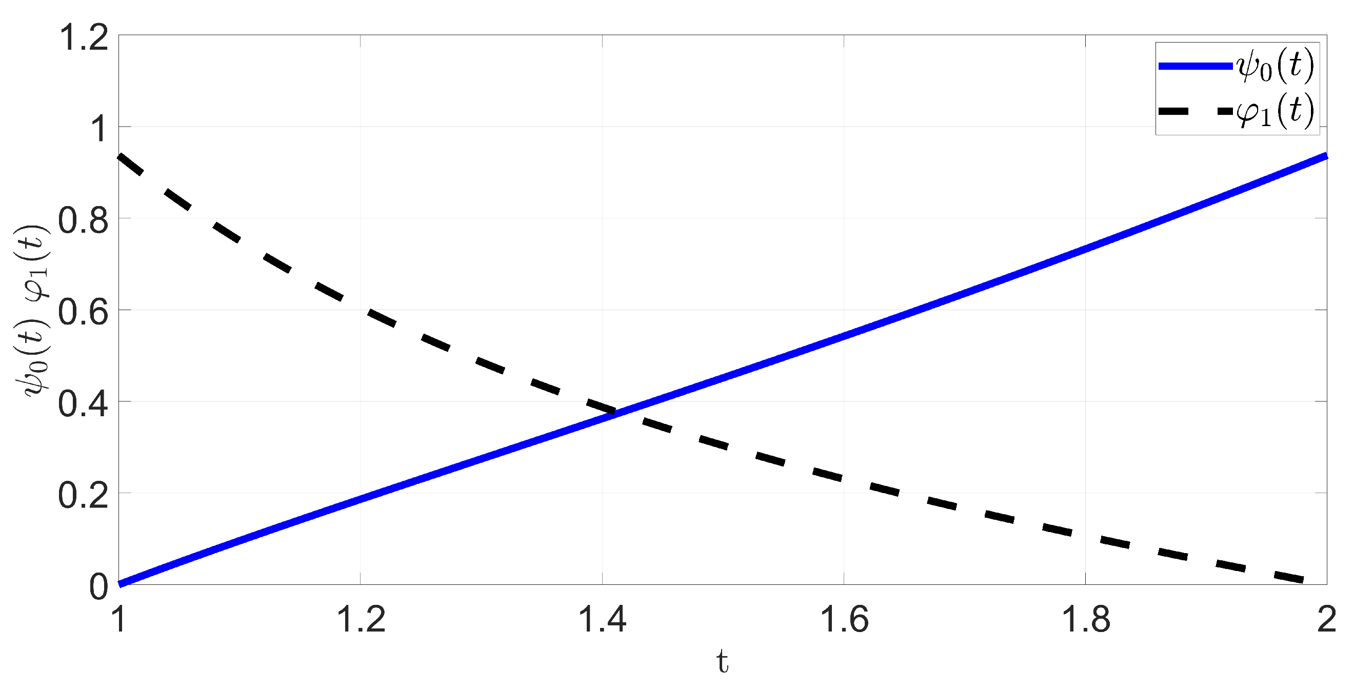
3.3. Case Study for a Singular ODE with a Piecewise Source Term

In this section, we demonstrate the effectiveness and robustness of the proposed exact scheme in the case of a regular singular ODE, which appears in several physical and mathematical problems based on Equation (1).

$$Lu\left(x\right)=-\frac{d}{dx}\left(x\frac{d}{dx}u\left(x\right)\right)+\frac{m^2}{x}u\left(x\right)=f\left(x\right)(0<x<\infty )$$

(33)

where $\kappa \left(x\right)=x$, $q\left(x\right)=\frac{m^2}{x}$, $m\in \mathbb{R},m\ne 0$ and the source term is a noncontinuous function at $x=1/2$ (in the Equation (34)).

$$f\left(x\right)=\left\{\begin{array}{cc}x,\hfill & \mathrm{if}x<\frac{1}{2}\hfill \\ {\displaystyle \frac{1}{x},}\hfill & \mathrm{if}\frac{1}{2}\le x\hfill \end{array}\right.$$

(34)

Equation (33) is a second order Cauchy–Euler type, singular-regular differential equation that has singularities at $x=0$ and $x\to \infty$. The aim of our case study is to show that the mathematical method presented in this paper is suitable for the effective treatment of singularities in addition to creating a solution for ODE Equation (33) with the boundary conditions defined in Equation (35). Furthermore, the exact scheme also handles the behavior of the source term robustly. In particular, the non-differentiable property of $f\left(x\right)$ does not cause any problems for the implementation of the method. Although the function $f\left(x\right)$ is non-differentiable, its integrals still exist; thus, the necessary calculations can be performed. We will examine how $u\left(x\right)$ behaves at the singular points of ODE (Equation (33)). To perform this, we will add new mesh points $a,b$ to exclude singularities and then obtain function $u\left(x\right)$ on the new mesh by using the results presented in Theorem 2. Next, we will examine how the solution can be modified into a form in which the solution also exists at the singular points of the ODE by taking the limits $a\to 0^{+},b\to \infty$.

In order to obtain the solution ($u\left(x\right)$) to Equation (33), we choose the Dirichlet boundary conditions as follows:

$${\mathfrak{B}}_D=\left\{u\left(a\right)=\alpha ,u\left(b\right)=\beta \right\}.$$

(35)

where $0<a\le 1/2$ and $1/2\le b<\infty$. The shape functions are

$${\psi }_0\left(t\right)=\frac{1}{2m}\left(\frac{t^m}{a^m}-\frac{t^{-m}}{a^{-m}}\right)$$

(36)

and

$${\phi }_1\left(t\right)=-\frac{1}{2m}\left(\frac{t^m}{b^m}-\frac{t^{-m}}{b^{-m}}\right)$$

(37)

Since functions ${\psi }_0\left(t\right)$ and ${\phi }_1\left(t\right)$ are solutions to Equations (3) and (4), respectively, they have the following properties: ${\psi }_0\left(a\right)=0$, ${\phi }_1\left(b\right)=0$ and ${\psi }_0^{\prime }\left(a\right)=\frac{1}{a}$ and ${\phi }_1^{\prime }\left(b\right)=-\frac{1}{b}$.

Figure 4 shows functions ${\psi }_0\left(t\right)$ and ${\phi }_1\left(t\right)$ with substitutions $a=1$, $b=2$ and $m=2$.

The local green functions in Figure 4 have the same properties as the functions in Figure 1, except that here the test function pair ${\psi }_0$ and ${\phi }_1$ are the only pairs on the entire interval $[a,b]$. Obviously, this difference does not affect either the mathematical properties of the functions, or their physical properties according to the continuity boundary conditions.

After obtaining $a_0$, $a_1$, $b_1$, $G_0$ and $H_1$ from ${\psi }_0\left(t\right)$ and ${\phi }_1\left(t\right)$ using the Equations (11)–(14) in Theorem 2, the fundamental recursive formula (Equation (10)) for $n=1$ inner point, and $x_0=x_{i-1}=a,x_1=x,x_{i+1}=x_2=b$ is simplified in the form in the Equation (38).

$$-a_0\alpha +b_{1}u\left(x\right)-a_1\beta =a_0{G}_0+a_1{H}_1.$$

(38)

After isolating $u\left(x\right)$ from the Equation (38) and a necessary simplification is carried out, the solution of the ODE (in Equation (33)) with the corresponding boundary conditions (in Equation (35)) is given by Equation (39).

$$\begin{array}{cc}\hfill u\left(x\right)& =\frac{a^m(b^{2m}-x^{2m})}{x^m(b^{2m}-a^{2m})}\alpha +\frac{b^m(x^{2m}-a^{2m})}{x^m(b^{2m}-a^{2m})}\beta +{\int }_a^{b}G(x,t)f\left(t\right)dt\hfill \end{array}$$

(39)

where

$$G(x,t)=\frac{1}{2m(b^{2m}-a^{2m})}\left\{\begin{array}{cc}{\displaystyle \frac{(b^{2m}-x^{2m})(t^{2m}-a^{2m})}{x^m{t}^m}}\hfill & a\le t\le x\le b\hfill \\ \\ {\displaystyle \frac{(b^{2m}-t^{2m})(x^{2m}-a^{2m})}{t^m{x}^m}}\hfill & a\le x\le t\le b\hfill \end{array}\right.$$

(40)

In the next step, we examine how the solution function $u\left(x\right)$ behaves at the singular points of the original ODE. The solution considers that the singular points are obtained by taking the limits $a\to 0^{+},b\to \infty$. We also consider the properties of the $f\left(x\right)$ to evaluate improper integrals. If $a\to 0^{+}$, the limit of $u\left(x\right)$ can be obtained from Equations (39) and (40) as follows when $m>0$:

$$\begin{array}{cc}\hfill \underset{a\to 0^{+}}{lim}u\left(x\right)& =\frac{x^m}{b^m}\beta +{\int }_0^{x}f\left(t\right)\left(\frac{(b^{2m}-x^{2m})t^m}{2m{x}^m{b}^{2m}}\right)dt\hfill \\ \hfill & +{\int }_x^{b}f\left(t\right)\left(\frac{(t^{2m}-b^{2m})x^m}{2m{t}^m{b}^{2m}}\right)dt\hfill \end{array}$$

(41)

Equation (41) is a significantly simplified form of Equation (39), which shows that the substitution has eliminated the $u\left(0\right)=\alpha$ Dirichlet boundary condition. Furthermore, it can be seen that at this point, when taking the limit $b\to \infty$, the convergence of improper integrals is fulfilled only for certain functions $f\left(x\right)$. In our case study, we chose a source term that fulfills the following condition:

$${\int }_0^{\infty }\frac{\left|f\right(t\left)\right|}{t^m}dt<\infty ,$$

(42)

The equation for free space is obtained as:

$$u_0\left(x\right)=\underset{b\to \infty }{lim}\left(\underset{a\to 0^{+}}{lim}u\left(x\right)\right)={\int }_0^{x}f\left(t\right){\left(\frac{t}{x}\right)}^{m}dt+{\int }_x^{\infty }f\left(t\right){\left(\frac{x}{t}\right)}^{m}dt$$

(43)

Now, we can substitute $f\left(x\right)$ (Equation (34)) into (43) and evaluate the integrals. Since $f\left(x\right)$ is piecewise, the solution will be (if $0<m\ne 2$).

$$u_0\left(x\right)=\left\{\begin{array}{cc}{\displaystyle \frac{x^2}{m^2-4}-\frac{2^m(8-3m)x^m}{8(m-2)m^2}}\hfill & 0\le x<\frac{1}{2}\hfill \\ \\ {\displaystyle \frac{1}{m^2}-\frac{2^{-m}(8+3m)x^{-m}}{8(m+2)m^2}}\hfill & \frac{1}{2}\le x\hfill \end{array}\right.$$

(44)

It is easy to notice that $u_0\left(x\right)$ satisfies the original ODE (Equation (33)). It is interesting to note that in the case of $m=2$, the denominator of the solution (at interval $0\le x<\frac{1}{2}$) becomes zero. It is also noticeable that the numerator of the same function also becomes zero for $m=2$. Therefore, instead of substitution, we can take the limit, which when evaluated with the L’Hospital rule, leads to the following result:

$$u_0\left(x\right)=\left\{\begin{array}{cc}{\displaystyle -\frac{1}{16}{x}^2(-9+4ln\left(2x\right))}\hfill & 0\le x<\frac{1}{2}\hfill \\ \\ {\displaystyle \frac{1}{4}-\frac{7}{256x^2}}\hfill & \frac{1}{2}\le x\hfill \end{array}\right.$$

(45)

Function $u_0\left(x\right)$ is bounded in the singular points of ODE, because

$$u_0\left(0^{+}\right)=0$$

(46)

and

$$\underset{x\to \infty }{lim}{u}_0\left(x\right)=\frac{1}{m^2}$$

(47)

is constant to any m. Figure 5 shows the graph of $u_0\left(x\right)$ for $m=1,2,3,4$.

As shown in Figure 5 and in Equations (44) and (45), function $u_0\left(x\right)$ is continuous and differentiable at $x=\frac{1}{2}$, even in the case of a discontinuous $f\left(x\right)$.

4. Conclusions

The application of the proposed scheme provides the opportunity to generate the values of the analytical solution that is obtained in grid points. This method can be easily implemented in different software environments (such as MATLAB, Maple, and Mathematica); thus, many physical problems can be modeled to avoid errors that are caused by the numerical approximations when using arbitrary grids. Currently, the most critical issue in the application of this scheme is to obtain the solution of a homogeneous equation, which may be challenging. Therefore, in future generalizations, we will consider the importance of providing a solution to this problem to complete the scope of the application areas. Furthermore, we generalize the concept presented in this paper by the application of the Sturm–Liouville theory, focusing on the symmetry of the local green functions and the gained advantageous properties.

The application of the exact scheme to Sturm–Liouville problems will represent a milestone in the research, that will complete the study of linear second-order ODEs. As a consequence, we will be able to concentrate our research activities on the symbolic treatment of nonlinear ODEs and inverse problems, as the main two motivating areas of the research group.

References

1. Regmi, R.P. Application of differential equation in L-R and C-R circuit analysis by classical method. Janapriya J. Interdiscip. Stud. 2017, 5, 114–123. [Google Scholar] [CrossRef] [Green Version]
2. Tai-Ran, H. Applied Engineering Analysis; John Wiley and Sons Ltd.: Hoboken, NJ, USA, 2018; ISBN 1119071208. [Google Scholar]
3. Simpson, M.J.; Lythe, G. (Eds.) Exact Solutions of Linear Reaction-Diffusion Processes on a Uniformly Growing Domain: Criteria for Successful Colonization. PLoS ONE 2015, 10, e0117949. [Google Scholar]
4. Al-Gwaiz, M. Sturm-Liouville Theory and Its Applications; Springer: London, UK, 2008; ISBN 978-1-84628-972-9. [Google Scholar]
5. Strang, G. Differential Equations and Linear Algebra; Wellesley-Cambridge Press: Cambridge, UK, 2015; ISBN 0980232791. [Google Scholar]
6. LeVeque, R.J. Finite Difference Methods for Ordinary and Partial Differential Equations; Society for Industrial and Applied Mathematics: Philadelphia, PA, USA, 2007; ISBN 978-0-89871-629-0. [Google Scholar]
7. Adison, H. Principles and Practice of Finite Volume Method; Clanrye International: New York, NY, USA, 2015; ISBN 978-1632404176. [Google Scholar]
8. Sauter, S.; Schwab, C. Boundary Element Methods; Springer: Berlin/Heidelberg, Germany, 2010; ISBN 978-3-540-68093-2. [Google Scholar]
9. Pepper, D.W.; Heinrich, J.C. The Finite Element Method; CRC Press: Boca Raton, FL, USA, 2017; ISBN 978-1498738606. [Google Scholar]
10. Anulo, A.A. Numerical Solution of Linear Second Order Ordinary Differential Equations with Mixed Boundary Conditions by Galerkin Method. Math. Comput. Sci. 2017, 2, 66–78. [Google Scholar] [CrossRef] [Green Version]
11. Cao, D. An Exponential Spline Difference Scheme for Solving a Class of Boundary Value Problems of Second-Order Ordinary Differential Equations. Discret. Dyn. Nat. Soc. 2020, 2020, 1–16. [Google Scholar] [CrossRef]
12. Mamadu, J.E.; Njoseh, I.N. Tau-Collocation Approximation Approach for Solving First and Second Order Ordinary Differential Equations. J. Appl. Math. Phys. 2016, 4, 383–390. [Google Scholar] [CrossRef] [Green Version]
13. Svantnerne Sebestyen, G.; Farago, I.; Horvath, R.; Kersner, R.; Klincsik, M. Stability of patterns and of constant steady states for a cross-diffusion system. J. Comput. Appl. Math. 2016, 293, 208–216. [Google Scholar] [CrossRef]
14. Kersner, R.; Klincsik, M.; Zhanuzakova, D.T. A competition system with nonlinear cross-diffusion: Exact periodic patterns. Rev. Real Acad. Cienc. Exactas Fis. Nat. Ser. A. Mat. 2022, 116, 187. [Google Scholar] [CrossRef]
15. Kaur, K.; Singh, G. An Efficient Non-Standard Numerical Scheme Coupled with a Compact Finite Difference Method to Solve the One-Dimensional Burgers’ Equation. Axioms 2023, 12, 593. [Google Scholar] [CrossRef]
16. Vrabel, R. Lower and Upper Solution Method for Semilinear, Quasi-Linear and Quadratic Singularly Perturbed Neumann Boundary Value Problems. Axioms 2023, 12, 154. [Google Scholar] [CrossRef]
17. Shukla, A.; Vedula, P. A hybrid classical-quantum algorithm for solution of nonlinear ordinary differential equations. Appl. Math. Comput. 2023, 442, 127708. [Google Scholar] [CrossRef]
18. Sari, Z.; Klincsik, M.; Odry, P.; Tadic, V.; Toth, A.; Vizvari, Z. Lumped Element Method Based Conductivity Reconstruction Algorithm for Localization Using Symmetric Discrete Operators on Coarse Meshes. Symmetry 2023, 15, 1008. [Google Scholar] [CrossRef]
19. Uhlmann, G. 30 Years of Calderón’s Problem, Seminaire Laurent Schwartz—EDP et Applications, Cellule MathDoc/CEDRAM, Séminaire Laurent Schwartz—EDP et Applications. 2012, pp. 1–25. Available online: http://eudml.org/doc/275764 (accessed on 24 June 2023).
20. Bondarenko, N.P. Inverse Spectral Problems for Arbitrary-Order Differential Operators with Distribution Coefficients. Mathematics 2021, 9, 2989. [Google Scholar] [CrossRef]
21. Argun, R.; Gorbachev, A.; Lukyanenko, D.; Shishlenin, M. On Some Features of the Numerical Solving of Coefficient Inverse Problems for an Equation of the Reaction-Diffusion-Advection-Type with Data on the Position of a Reaction Front. Mathematics 2021, 9, 2894. [Google Scholar] [CrossRef]
22. Samarskii, A.A. The Theory of Difference Schemes; CRC Press: Boca Raton, FL, USA, 2001; ISBN 0-82470468-1. [Google Scholar]
23. Delkhosh, M. The Conversion a Bessel’s Equation to a Self-Adjoint Equation and Applications. World Appl. Sci. J. 2011, 15, 1687–1691. [Google Scholar]
24. Kiguradze, I.T.; Shekhter, B.L. Singular boundary-value problems for ordinary second-order differential equations. J. Sov. Math. 1988, 43, 2340–2417. [Google Scholar] [CrossRef]
25. Kiguradze, T. On solvability and unique solvability of two-point singular boundary value problems. Nonlinear Anal. Theory Methods Appl. 2009, 71, 789–798. [Google Scholar] [CrossRef]
26. Kiguradze, I.T.; Kiguradze, T.I. Conditions for the well-posedness of nonlocal problems for second-order linear differential equations. Differ. Equ. 2011, 47, 1414–1425. [Google Scholar] [CrossRef]
27. Vizvari, Z.; Sari, Z.; Klincsik, M.; Odry, P. Exact schemes for second-order linear differential equations in self-adjoint cases. Adv. Differ. Equ. 2020, 2020, 497. [Google Scholar] [CrossRef]
Figure 1. Graphs of local green functions ψ 0 ( x ) , ψ 1 ( x ) , ψ 2 ( x ) , and ψ 3 ( x ) (with solid lines) and φ 1 ( x ) , φ 2 ( x ) , φ 3 ( x ) , and φ 4 ( x ) (with dotted lines) (defined in the Equation (31) using the partitioning in Equation (30)) on the interval [ 0 , 2 ] ( n = 3 ).
Axioms 12 00633 g001
Figure 2. The results of the case study: u ( x ) is denoted with blue line, while u i , the result obtained in the i t h grid point, is denoted with black dots.
Axioms 12 00633 g002
Figure 3. Solving the case study with discontinuous κ ( x ) (in terms of Equations (26) and (27) and q ( x ) = 2 ) for different mesh resolutions ((a) n = 15 , (b) n = 50 , (c) n = 100 ).
Axioms 12 00633 g003
Figure 4. Graph of local green functions ψ 0 ( t ) and φ 1 ( t ) if a = 1 , b = 2 and m = 2 .
Axioms 12 00633 g004
Figure 5. The solution u 0 ( x ) (in Equation (44)) of the case study for a singular ODE with a piecewise source term ( m = 1 , 2 , 3 , 4 ).
Axioms 12 00633 g005
Disclaimer/Publisher’s Note: The statements, opinions and data contained in all publications are solely those of the individual author(s) and contributor(s) and not of MDPI and/or the editor(s). MDPI and/or the editor(s) disclaim responsibility for any injury to people or property resulting from any ideas, methods, instructions or products referred to in the content.