Abstract
In this research, we propose fourth-order non-uniform Hermitian differencing with a fifth-order adaptive time integration method for pricing system of free boundary exotic power put options consisting of the option value, delta sensitivity, and gamma. The main objective for implementing the above scheme is to carefully account for the irregularity in the locality of the left corner point after fixing the free boundary. Specifically and mainly, we stretch the performance of our proposed method threefold. First, we exploit the non-uniform fourth-order Hermitian scheme to locally concentrate space grid points arbitrarily close to the left boundary. Secondly, we further leverage the adaptive nature of the embedded time integration method, which allows optimal selection of a time step based on the space grid point distribution and regional variation. Thirdly, we introduce a fourth-order combined Hermitian scheme, which requires fewer grid points for computing the near boundary point of the delta sensitivity and gamma. Another novelty is how we approximate the optimal exercise boundary and its derivative using a fifth-order Robin boundary scheme and fourth-order combined Hermitian scheme. Our proposed method consistently achieves reasonable accuracy with very coarse grids and little runtime across the numerical experiments. We further compare the results with existing methods and the ones we obtained from the uniform space grid.
Keywords:
power options; optimal exercise boundary; compact finite difference scheme; 5(4) Dormand–Prince embedded pairs MSC:
65N06; 65M50; 35R35
1. Mathematical Model
In this research, we propose a high-order non-uniform space and adaptive time stepping scheme for pricing a system of free fixed-boundary exotic power put options pricing models. Specifically, the high-order schemes in space and time are obtained from the non-uniform fourth-order Hermitian differencing and Runge–Kutta adaptive time integration based on 5(4) Dormand–Prince embedded pairs [1]. We formulate our solution framework as a free boundary problem which approximates, simultaneously, the optimal exercise boundary, option value, and Greeks. To this end, we first revisit the original Black–Scholes equation. Let us consider non-dividend-paying put options written on an underlying asset with price , strike price K, and time-to-maturity T; the free boundary partial differential equation is then given as
The asset price is driven by geometric Brownian motion , given as
Here, is a standard Brownian motion. represents the volatility, and r is the interest rate. Let us consider as a new underlying asset, with m representing the power of the option value. Applying Itô’s formula, and under risk-neutral probability , we then obtain
with the governing differential equation given as below as
In this context, . Kim [2] classified power options as standard power options, capped power options, and powered options. For standard power options, the payoff is given as
Here, . For the capped power options, we also have the following
Here, , and L represents a pre-defined, capped level. For the powered option, we also provide the following:
Lee et al. [3] and Topper [4] described an option representing the payoff in (7) as symmetric power options. Heynen and Kat [5] further presented power options with a more generalized payoff given as
Here, we focus on the power payoff function presented in the work of Nwozo and Fadugba [6] and Lee [7], which is as follows
This is similar to the standard power options in (5), except that K is fixed with . It is also known as an asymmetric power option [4]. Lee et al. [3] and Wang [8] described a generalization of such options in (9) as polynomial options, given as
Power options are high-risk, high-reward options. They leverage a magnified position compared to vanilla options due to the non-linear nature of the payoff. Small changes in the asset price can lead to a substantial change in the price of the option based on the power term m. Therefore, for a security that it is expected to rise or fall, the call option holder is bound to incur substantial gains or losses [9,10]. As described in the work of Kim [2] and Huang et al. [9], power options are widely traded in the financial market and have been issued in some countries in the form of polynomial power options [5] and capped FX power options [4].
In the American style framework with , the governing differential equation in (4) is then reduced to a free boundary partial differential equation as shown below
The boundary and the initial condition are further given as shown below
To fix the free boundary and remove the convective term that could further introduce error, we then implement a Landau transformation and further take the derivative as given below
Hence, the transformed system of nonlinear American options pricing model consisting of option value, delta sensitivity, and gamma is given below
When and , we need to substitute the left boundary values of the option value with the first derivative in time and space to (17), from which we obtain
Several authors have proposed methods for solving exotic power options in both European- and American-style frameworks using both integral and differential solution forms. Okelola et al. [10] solved the power options model in the European framework using the Lie group method. Heynen and Kat [5] presented power options in the European framework with a more generalized polynomial payoff. The authors then considered standard power options, generalized power options, and parabola options. Kim [2] solved the power options in the European framework based on the regime switching model. Rao [11] solved the Asian power options under fractional Brownian motion. Esser [12] derived a compact formulation for general payoff and applied it to standard power options, powered options, and capped power options under stochastic volatility. Kim et al. [13] solved the exotic power options under the Heston volatility model. Blenman et al. [14] solved a power exchange options written on a zero-coupon bond in a stochastic interest rate framework. Ha et al. [15] solved a time power option under stochastic volatility.
Lee [7] numerically solved a non-dividend-paying American-style power option PDE model as a free boundary problem with a second-order finite difference scheme. To the best of our knowledge, only this author has attempted to solve such an exotic option PDE model as a free boundary problem with a low-order scheme. Our main objective here is to propose a high-order, fast, stable, and accurate non-uniform and adaptable numerical scheme that solves a system of American-style exotic power option pricing models as a free boundary problem. These systems of free boundary PDEs will solve the option value, delta sensitivity, gamma, and optimal exercise boundary simultaneously. To the best of our knowledge, we are the first to propose such a high-order scheme, non-uniform in space and adaptive in time, for solving systems of free boundary exotic power option pricing PDEs that simultaneously approximate the option value, Greeks, and the free boundary.
The remaining sections of this work are organized as follows. In Section 2, we introduce a fourth-order non-uniform compact finite difference scheme and fifth-order adaptive time integration based on 5(4) Dormand–Prince, Runge–Kutta embedded pairs [1] for solving the free boundary exotic power options pricing problem on a locally refined space grid. We verify the performance of this non-uniform and adaptive scheme and present our numerical results in Section 3. We further compare with the existing method and conclude our study in Section 4.
2. Numerical Methods
In this section, we present the numerical methods for computing the value function, Greeks, and the optimal exercise feature of the American power put options. The numerical computation was carried out in the domain . Here, we replace the infinite space domain with the far-field boundary . This is because, for the put options, the value function vanishes rapidly as we move further away from the right boundary (out of the money). The space–time grid and its node points are described below
We further label the numerical approximation of the option price, delta sensitivity, gamma, and the optimal exercise boundary as , , and , with
Stable treatment of the variation at the left corner point and computation of the optimal exercise boundary and its derivative with precision are at the heart of this research work, and both objectives are intertwined. Moreover, the precise computation of the optimal exercise boundary and its first derivative will influence the accuracy of the option value and the hedge sensitivity. The secondary intention here is to understand how we can use a few grid points to achieve greater accuracy by feeding more of those grid points to the locality of the left corner point. To this end, we seek some leverage and control in the locality of the left corner point of the grid such that we can manipulate the space grid distribution in that neighborhood and further allow the fifth-order time integration method based on Dormand–Prince, Runge–Kutta embedded pairs [1] to select the optimal time step at each time level that adapts well to the regional variation and space grid distribution. The adaptive attribute of the embedded time stepping plays well in our favor here by allowing us to initialize our proposed method with arbitrary time steps and fixed step sizes h, thus circumventing the stability challenge associated with explicit time integration schemes. The strategic implementation is described fully in the subsections of this section.
2.1. Fourth-Order Non-Equidistant Hermitian Differencing on a Locally Refined Grid
In this subsection, we present a high-order numerical scheme that enables grid refinement about the locality of the left corner point by introducing local mesh refinement results in a non-uniform grid. Hence, the conventional fourth-order compact scheme is no longer applicable. To this end, we introduce the non-equidistant fourth-order Hermitian differencing presented in the work of Shukla and Zhong [16] and Shukla et al. [17] for discretizing interior nodes as given below
with
Refining grids in the locality of the optimal exercise boundary point gives us some advantages, which will be described below. It allows us to use more nodal points very close to when computing the optimal exercise boundary. We will exploit this feature in a more strategic way in this subsection.
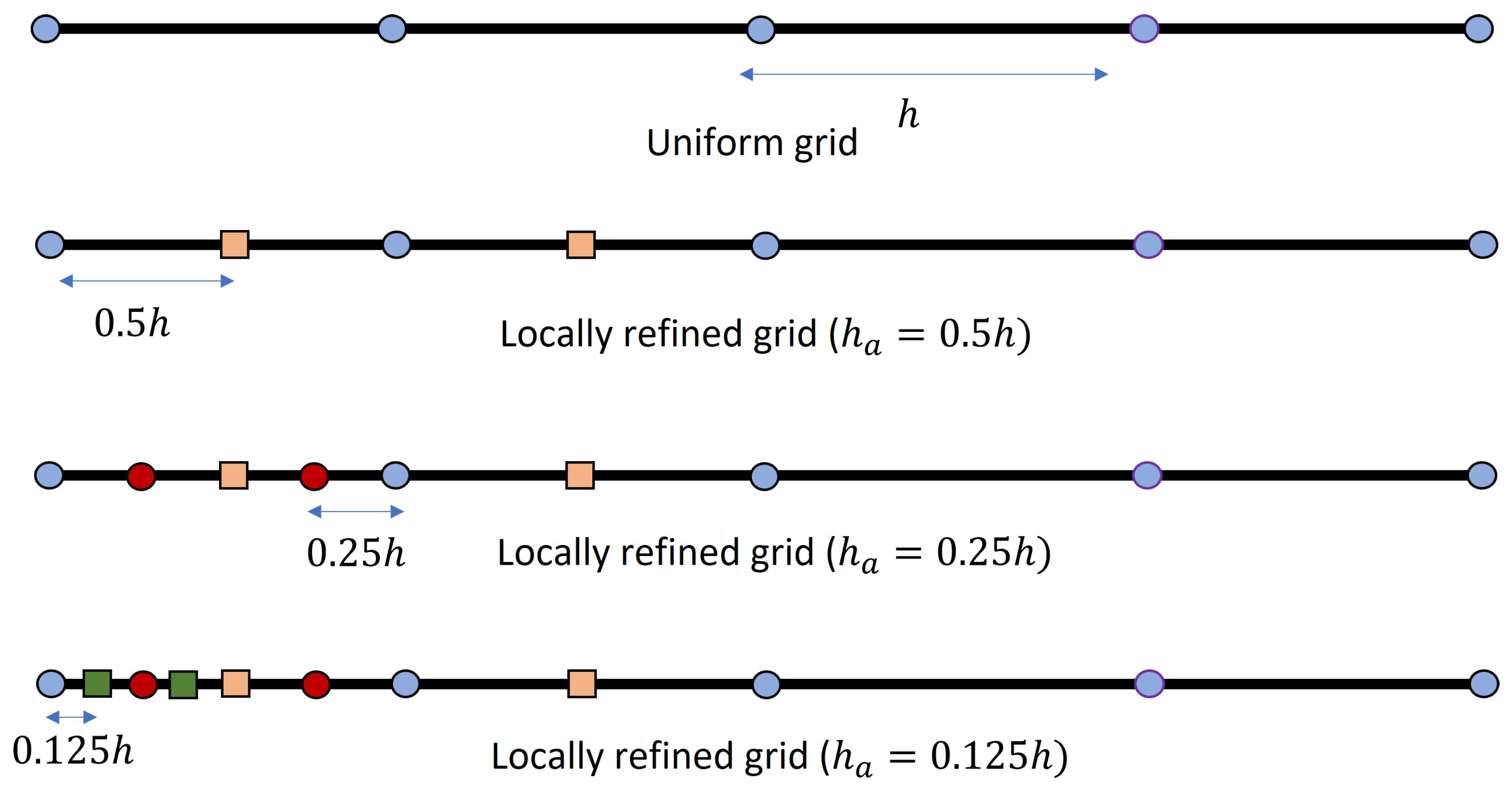
Here, we will first establish a uniform grid and then manually add a few extra grid points very close to the left boundary point. We will use the near-left boundary grid points to initialize the first derivative of the optimal exercise boundary and further compute the optimal exercise boundary and its first derivative after each successive function evaluation stage with the fifth-order Runge–Kutta embedded time integration method based on Dormand–Prince pairs. This implementation will both allow us to use points very close to the left boundary to approximate the optimal exercise boundary and its derivative and enable a locally refined grid in the left corner, where inherent irregularities and variation reside. Here, we delicately add these few grid points in such a way that the points we use for computing the free boundary and the near boundary discrete values are both very refined and equidistant, even though the grid is globally non-uniform. For a description, please see Figure 1. For a similar implementation for solving the options pricing problem with a high-order compact scheme, please see the work of Chen et al. [18] and Lee and Sun [19].
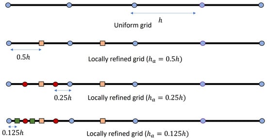
Figure 1.
Uniform and locally refined space grids ().
For the near boundary scheme, i.e, , we will consider fourth-order combined compact finite difference schemes for approximating the solution of the option value as given below
We point out that the fourth-order, one-sided, non-combined compact scheme given below
can also be used as the near boundary scheme for the option value as presented in the work of Zhao and Corless [20] and Nwankwo and Dai [21]. However, we observe that, for uniform implementation, the fourth-order combined compact scheme in (33) provides more reasonable accuracy, although the discrepancy when compared with (34) is not substantial. We imagine that the reason could be that we use fewer grid points for approximation. The availability of discrete solutions for hedge sensitivity also works in our favor here. Moreover, for the non-uniform grid, we are trying to avoid using more grid points to account for the near boundary scheme based on the slight uniformity we achieve near the left boundary. Any selected grid points for accounting for the near boundary value must fall within the local uniform domain, even though our space grid is globally non-uniform. Hence, in the Section 3, we consider only (33). Furthermore, for the delta sensitivity, we use a different fourth-order near boundary combined compact finite difference scheme by considering the following lemma
Lemma 1.
Assume that ; we have
Proof.
We observed after deriving this fourth-order combined compact scheme in (35) that the latter had already been presented and used in the work of Abrahamsen and Fornberg [22] and, as such, we recognized the need to acknowledge their work here. The high-order scheme in (35) allows us to use the discrete value of the option value to approximate the near boundary value of delta, thereby reducing sensitivity. Moreover, fewer nodal values of the higher derivatives are used when deriving the near boundary scheme for the delta sensitivity, as shown in (35). It is worth mentioning that, for the delta sensitivity, the novel near-boundary fourth-order combined compact scheme in (35) is much more suitable and provides a more accurate result when compared with (34). In the uniform case, the condition number of the discrete matrix system generated with (34) is larger when compared with (35). Similarly, the near boundary value for the gamma is approximated as follows
More importantly, we present below a high-order Robin boundary scheme for approximating the optimal exercise boundary and its derivative after each function evaluation stage with the high-order embedded time integration method. To this end, we consider the following lemma
Lemma 2.
Assume that ; we have
Proof.
Let , 1,2,3. To prove the lemma in (40), we first present the Taylor series expansion around as follows
Multiplying (41) by 8 and subtracting from (42), we obtain
Multiplying (42) by and subtracting from (43), we obtain
Multiplying (44) by and subtracting from (42) with some re-arrangement, we obtain (40), and the proof is completed. □
The high-order scheme above will enable us to approximate the optimal exercise boundary and its first derivative in time with better precision. If we consider value matching, smooth pasting, and the implied second derivative boundary conditions
we obtain
For simplicity, let
Hence,
Equation (50) approximates the optimal exercise boundary after each function evaluation based on Runge–Kutta embedded pairs that are described in the following subsection. Equation (50) is also used to formulate an analytical approximation for initializing and further correcting the first derivative of the optimal exercise boundary. To this end, we take the derivative of (48) with respect to time and obtain the following
Due to the time-dependent coefficient present in our model, the first derivative of the optimal exercise boundary needs to be computed with precision, especially very close to the expiration. Here, we derive a novel high-order analytical approximation for the initialization (prediction) of the first derivative of the optimal exercise boundary at each time level, which will be subsequently corrected from the solutions of the Runge–Kutta pairs at each stage of function evaluation using (51). To this end, we recall the fourth-order combined compact finite difference presented as given below
For simplicity, let
Furthermore, considering the PDE governing the fixed free boundary American options, we obtain the following
Further simplification reveals that
with
It is important to observe that establishing a system of free boundary PDEs consisting of the option value and hedge sensitivity is very useful here. Not only does it enable us to deal with the convective term that could further introduce error and allow simple implementation of the fourth-order compact scheme, but we also use the discrete solution of the delta sensitivity for predicting the initial value of the first derivative of the optimal exercise boundary for each time level. Furthermore, computing the Greeks simultaneously with the option value and optimal exercise boundary using a fourth-order compact operator presents some benefits that could be substantial if the computational cost is very low. We hope to demonstrate extensively in the Section 3 that our implementation holds such an advantage. For the rest of the interior points for the option value and delta sensitivity, we use the same fourth-order compact scheme presented in (29). Hence,
with , , , , , , and , given as:
With the discrete matrix system above, we then obtain the semi-discrete system for the option value and hedge sensitivity as follows
Remark 1.
It is worth acknowledging here the recent work of [23], where the authors implemented a high-order non-uniform Hermitian scheme for solving the fractional Black–Scholes model. The non-uniform high-order scheme proposed by the authors in their paper can also be used in this research work.
2.2. 5(4) Dormand–Prince, Runge–Kutta Embedded Time Integration Method
As mentioned in the previous subsection, at each time level (and more importantly, when ), the first derivative of the optimal exercise boundary is initialized (predicted) as given below.
- Preliminary stage:The numerical procedure for the implementation of adaptive time stepping at each time level based on the 5(4) Dormand–Prince, Runge–Kutta embedded time integration method is described below.
- First stage:
- Second stage:
Third stage:
Fourth stage:
Fifth stage:
Sixth stage:
Seventh stage:
Here, , , and are obtained from the fifth-order Runge–Kutta integration scheme, which will represent the numerical approximation of the optimal exercise boundary, option value, and hedge sensitivity. Moreover, , , and are fourth-order accurate in time and will be used in conjunction with the solution from the fifth-order scheme to establish an error threshold for the selection of the optimal time step based on the regional variation and grid point distribution. For brevity, we skip further explanation. Please see the work of Nwankwo and Dai [21,24,25], where the author describes the implementation of these embedded pair(s) for solving the American options pricing model that involves coupled systems of diffusive–convective–reaction PDEs on a uniform space grid.
3. Numerical Experiment
In this section, we investigate the efficiency of our implementation and compare its performance with some of the existing methods in the literature, as well as with the results obtained with the uniform fourth-order compact scheme and 5(4) Dormand–Prince embedded pairs. Numerical experiments were carried out on a workstation with a 12th Gen Intel(R) Core(TM) i7-12700H at 2.30 GHz on a 64-bit Windows 11 operating system. Furthermore, the MATLAB programming language was used for numerical experiments and visualization. For convenience, we label our methods as follows
- DPC-Uniform: Fourth-order compact scheme with 5(4) Dormand–Prince embedded pairs on an equidistant space grid;
- DPC-Loc1: Fourth-order compact scheme with 5(4) Dormand–Prince embedded pairs on a locally refined space grid ().
- DPC-Loc2: Fourth-order compact scheme with 5(4) Dormand–Prince embedded pairs on a locally refined space grid ().
- DPC-Loc3: Fourth-order compact scheme with 5(4) Dormand–Prince embedded pairs on a locally refined space grid ().
In all the examples in this section, we conduct our experiment with very coarse grids. is the minimum step size we use for computing our numerical solutions. Furthermore, , , and represent the smallest step size in the space grid, which represents the step size of the local uniform domain close to the left corner point in the non-uniform grids for DPC-Loc1, DPC-Loc2, and DPC-Loc3, respectively. The reason for conducting our experiment with a very coarse grid is to better understand if there are significant impacts our mesh refinement strategies could have on the solution accuracy, optimal time selection, and computational speed.
3.1. Investigating Solution Accuracy on Both Uniform and Non-Equidistant Space Grids with Unit Power Terms
In this subsection, we first consider a case for the power put option where the power term . When , we are simply investigating the vanilla American put options pricing problem. Here, we want to verify the performance of the presented method in terms of solution accuracy and computational runtime on both uniform and non-equidistant space grids with adaptive time stepping techniques. With a non-equidistant grid, we investigate the impact of local refinement and coordinate transformation on the solution accuracy and runtime in seconds using very coarse grids. To this end, we first consider the example presented in the work of Nwankwo and Dai [21] with the parameter shown in Table 1.

Table 1.
First numerical data.
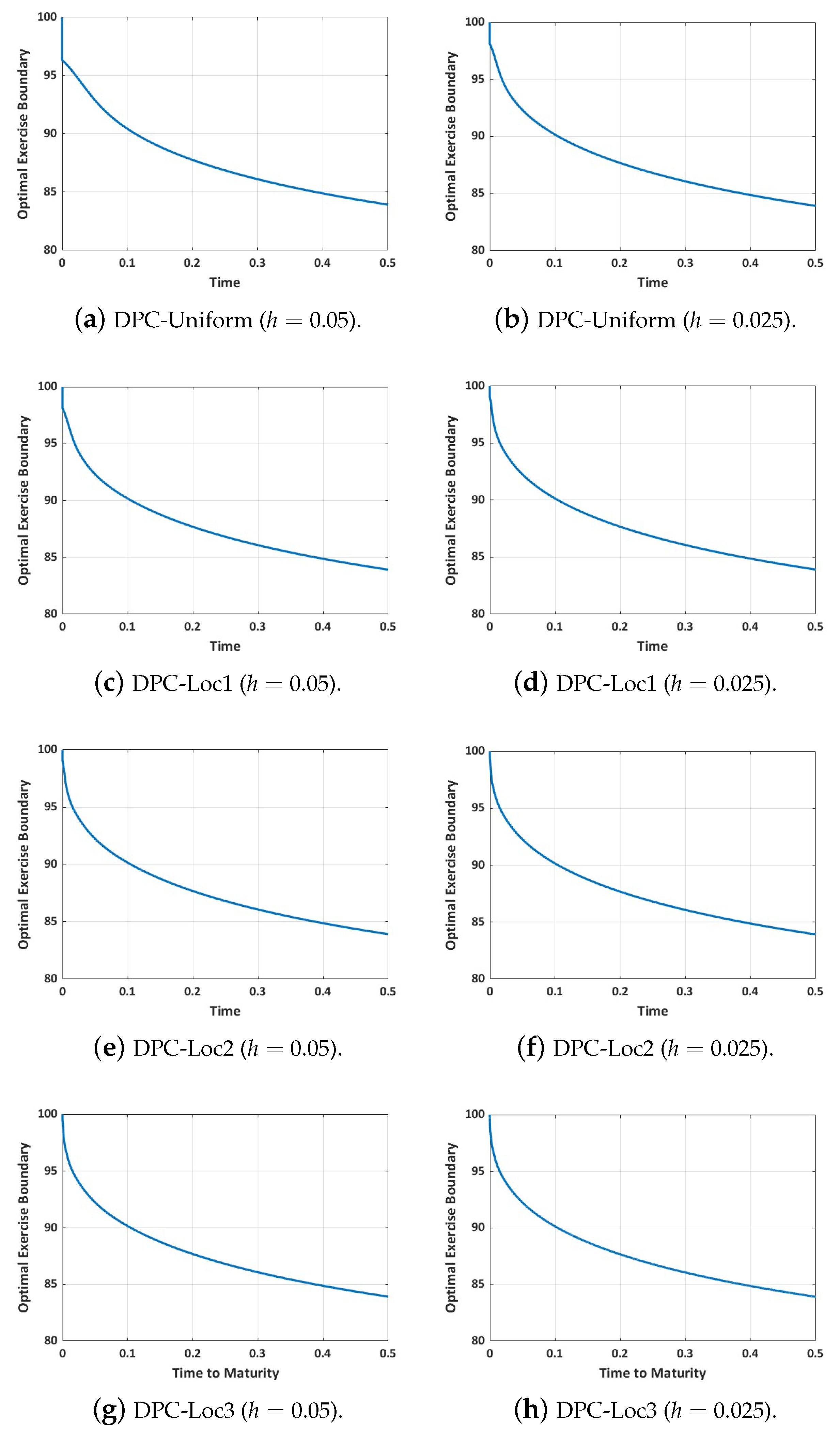
Here, we will use the numerical data above to investigate the solution accuracy of the optimal exercise boundary using both uniform and non-equidistant grids. Our experiment for this example is conducted on very coarse grids ( and ). The plot profile of the optimal exercise display is shown in Figure 2. In Table 2 and Table 3, we present the numerical approximation when with a runtime in seconds. Here, the runtime in seconds is defined as the time required to run the whole code from initialization to visualization. The benchmark solution is obtained from a sixth-order compact finite difference scheme with a third-order Runge–Kutta adaptive time integration method and free boundary improvement [25]. A step size of is used to obtain the benchmark value.
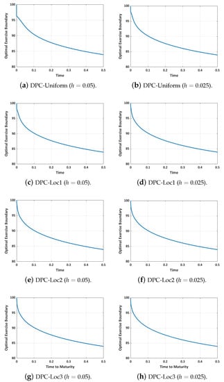
Figure 2.
Plot of the optimal exercise boundary with uniform and non-uniform Hermitian scheme .

Table 2.
Comparing the optimal exercise boundary and runtime in seconds (). is the benchmark value.

Table 3.
Comparing the runtime in seconds.
We observe from Figure 2 the importance of the local mesh refinement as it improves accuracy close to the left corner point where and . In Figure 2, for instance, with a uniform grid, when , the optimal exercise boundary is not very smooth close to the payoff. However, with locally refined grids, especially with DPC-Loc2 and DP-Loc3, we observe that the optimal exercise boundary is very smooth with , thus establishing the importance of refining the grid at the left corner point. Moreover, the scheme with a locally refined grid, as shown in Table 4, presents the most accurate result when compared with the one obtained from the uniform grid. Another advantage of the local mesh refinement as presented here is that only a few grid points are introduced while retaining the uniformity of the grid in most regions.

Table 4.
Initializing with varying initial time step and fixed step size ( and ).
Next, we establish that our proposed methods can be implemented with arbitrary step sizes and time steps, which is an important feature of the Runge–Kutta embedded time integration method. To this end, we fix and initialize with varying initial time steps and . We display the result in Table 4.
We observe from Table 4 that our proposed method is well-adapted to fixed step size h and to varying initial time step , and that this provides consistent and reasonable approximation for both large and small time steps. This is because the time integration scheme selects an optimal time step at each time level adaptively based on regional variation and grid point distribution. Hence, the choice of initialization for the time step does not matter and has no significant implication.
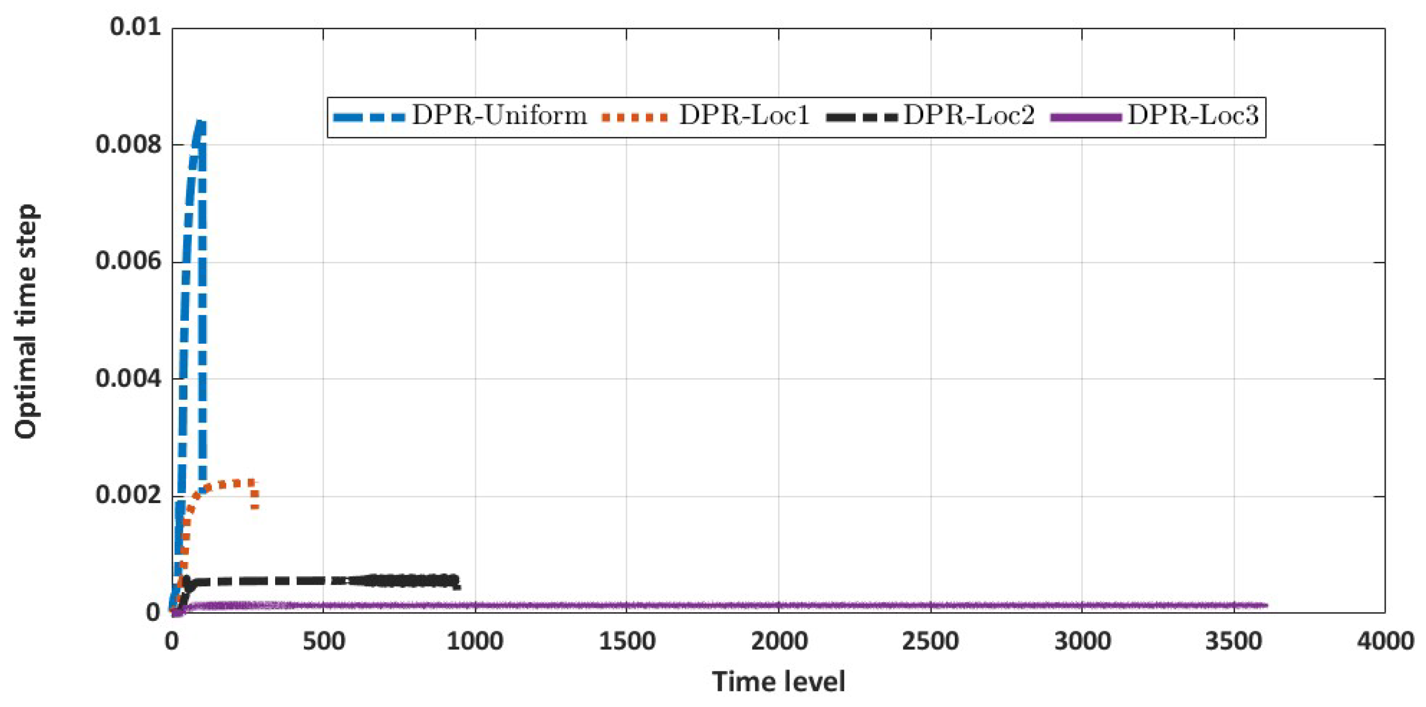
Finally, for this example, to better understand the impact of the grid distribution on the optimal time selection at each time level, we display the time stepping profile based on the uniform and non-equidistant grid distribution in Figure 3 with a step size of and . We observe that the time stepping is very small close to the payoff, which is expected based on the adaptability of our numerical scheme and the inherent irregularity that is more pronounced close to the payoff. Furthermore, we observe from Figure 3 that if we introduce more grid points in the locality of the left corner point, as can be observed from DPC-Loc1, DPC-Loc2, and DPC-Loc3, the time step for a fixed time level is smaller when compared with the uniform space grid distribution. However, from Table 3, we observe that the overall impact on the total runtime is insignificant when compared with the solution accuracy.
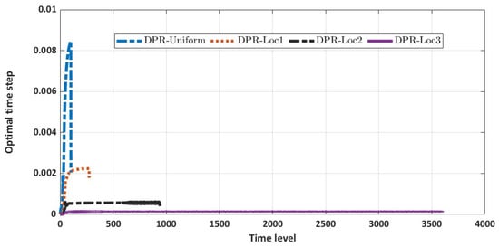
Figure 3.
Plot of the optimal time stepping for each time level ( and ).
In the second example, we will focus on option value and delta sensitivity. Here, we consider the example in the work of Bunch and Johnson [26] and Gutiérrez [27] with the following parameters displayed in Table 5.

Table 5.
Second numerical data.
The benchmark value used in their work was obtained from the binomial tree method with 10,000 steps. Here, we consider the numerical solution of the option value and delta sensitivity with a very coarse grid () and compare the performance of the uniform and non-equidistant space-grid implementation with the benchmark value. We display the results in Table 6 and Table 7.

Table 6.
Comparing the option value with varying strike price (, ).

Table 7.
Comparing the delta sensitivity with varying strike price (, ).
From Table 6 and Table 7, we observe reasonable solution accuracy for both the option value and delta sensitivity when compared with the binomial method. The interesting part is that reasonable solution accuracy was obtained with the non-equidistant space grid, which is closer to the benchmark value when compared with the results from the uniform grid. Achieving such solution accuracy on very coarse grids as described in Table 6 and Table 7 further validates the importance of our local mesh refinement strategy.
Remark 2.
It is worth mentioning that the approximation in the first and second examples involves only two system of PDEs in (17) and (18) consisting of the option value and delta sensitivity. The error threshold for selecting the optimal time step is established with the difference in the solution of the optimal exercise boundary, option value, and delta sensitivity for these examples based on the Runge–Kutta pairs. Moreover, the reported runtime in seconds only accounts for both PDEs. In the last example below, we consider the three systems of PDEs in (17)–(19) when accounting for gamma.
In this last example for this subsection, we investigate the importance of our proposed method in approximating gamma. Consider the example in the work of Tangman et al. [28] given in Table 8.

Table 8.
Third numerical data.
The differential and semi-discrete equations in (17), (18), (59), and (60) governing the option value and delta sensitivity are not coupled with that of their gamma counterpart. Hence, the investigation for gamma is done separately in this example. Here, we include the three PDEs in (17)–(19) and the three semi-discrete PDEs in (59)–(61). For the error threshold, which we establish for the optimal time step at each time level, we use maximum error obtained from the difference of the solutions of the optimal exercise boundary, option value, delta sensitivity, and gamma from the Runge–Kutta pairs as follows:
Here, . The optimal time step is selected if and if the true solutions are , , , and are selected. We observe that including the error from gamma in establishing the optimal time step ensures a stable and non-oscillatory solution for gamma. The important part, as we see in the result below, is that we can achieve reasonable solution accuracy with a large tolerance and very coarse grids, provided we include the error term from gamma when accounting for the optimal time step. Our main interest for this last example is to understand if we can achieve reasonable accuracy and little computational runtime with our local grid refinement. Furthermore, we also want to investigate how the local grid refinement impacts the solution accuracy and runtime in seconds. Here, our runtime in seconds includes the time it takes to run the whole code (approximate the early exercise boundary, option value, delta sensitivity, and gamma), excluding initialization to visualization.
To this end, we present the solution accuracy of the gamma obtained with our proposed method and compare our result from the non-equidistant space grid with the binomial tree method [29], which serves as benchmark value. For the non-equidistant grid, we consider DPC-Loc2. The binomial tree method is obtained with 15,001 steps as reported in the work of Tangman et al. [28]. Because of the high accuracy we observed from the gamma solution, we only consider very coarse grids with , , and . The results are displayed in Table 9, Table 10 and Table 11.

Table 9.
Gamma solution with DPC-Loc1 ().

Table 10.
Gamma solution with DPC-Loc2 ().

Table 11.
Gamma solution with DPC-Loc3 ().
The importance of our local mesh refinement is very visible in Table 9, Table 10 and Table 11. We observe that our solution accuracy is very close to the benchmark with a very coarse grid. More importantly, however, as we introduce few more grid points to the grid from DPC-Loc1-DPC-Loc3, the solution accuracy improve substantially. It is easy to see that we have achieved a result that is the same in most cases as the benchmark value, even with a very coarse grid () using DPC-Loc3. This important gain will be very useful in high-dimensional models due to space complexity. In general, very little computational time is required to approximate the early exercise boundary, option value, delta sensitivity, and gamma simultaneously with the locally refined grid.
Finally, to see the importance of including the error term in the optimal time step equation presented in (63)–(65), we call the implementation in the latter Scenario 1. For Scenario 2, we remove the error term for gamma from (63)–(65) and compute the gamma. To ensure an adequate result comparison for Scenario 2, we compute the result with very small and very large . The results are displayed in Table 12 and Table 13.

Table 12.
Gamma solution with DPC-Loc3 ().

Table 13.
Gamma solution with DPC-Loc3 ().
From Table 12 and Table 13, we observe that the solution accuracy for Scenario 2 is quite unreasonable with when compared with Scenario 1. However, the result of Scenario 2 starts stabilizing as we reduce the tolerance, which can be observed with . Moreover, increasing the tolerance will impact the computational cost. Hence, we can conclude that, to enable better estimation of the optimal exercise boundary, option value, delta sensitivity, and gamma from the three systems of PDEs consisting of the option value, delta sensitivity, and gamma, it might be ideal to include the error term associated with the four solutions as described in (63)–(65).
3.2. Investigating Solution Accuracy on Both Uniform and Non-Equidistant Space Grids with an Arbitrary Power Term
Here, we consider the power put options pricing problem with an arbitrary power term m and also consider the three systems of fixed free boundary PDEs in (17)–(19) and their discrete systems in (59)–(61). We verify the performance of our proposed method for solving such a model. By implementing an adaptive scheme, we have circumvented the stability challenges. We now focus more on understanding how varying m impacts the adaptive selection of time steps and the local mesh refinement strategy while presenting the numerical solutions. We carry out the whole experiment here with DPC-Loc2 because it presented more optimality in terms of computational time and solution accuracy in the previous subsection. Further, our experiment here is done with a very coarse grid and .
Few research studies exist that solve free boundary power options. Consider the example in the work of Lee [7] with the parameters as described in Table 14 below.

Table 14.
Fourth numerical data.
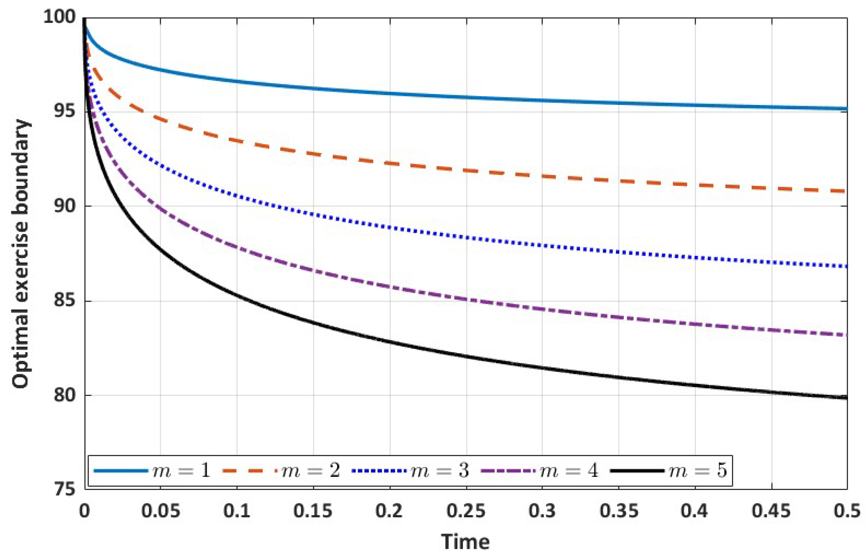
First, we compute the optimal exercise boundary for varying power term 1, 2, 3, 4, and 5, similar to the one presented in Lee’s [7] paper, and display the results in Figure 4. We observe that, for a fixed time, the optimal exercise boundary decreases as the power term m increases. This is further reflected in the value of the optimal exercise boundary with varying power term m as presented in Table 15. Our plot also closely resembles the one presented in the work of Lee [7].
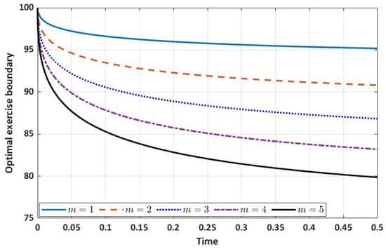
Figure 4.
Optimal exercise boundary with varying power term m.

Table 15.
Optimal exercise boundary with varying power term m (, ).
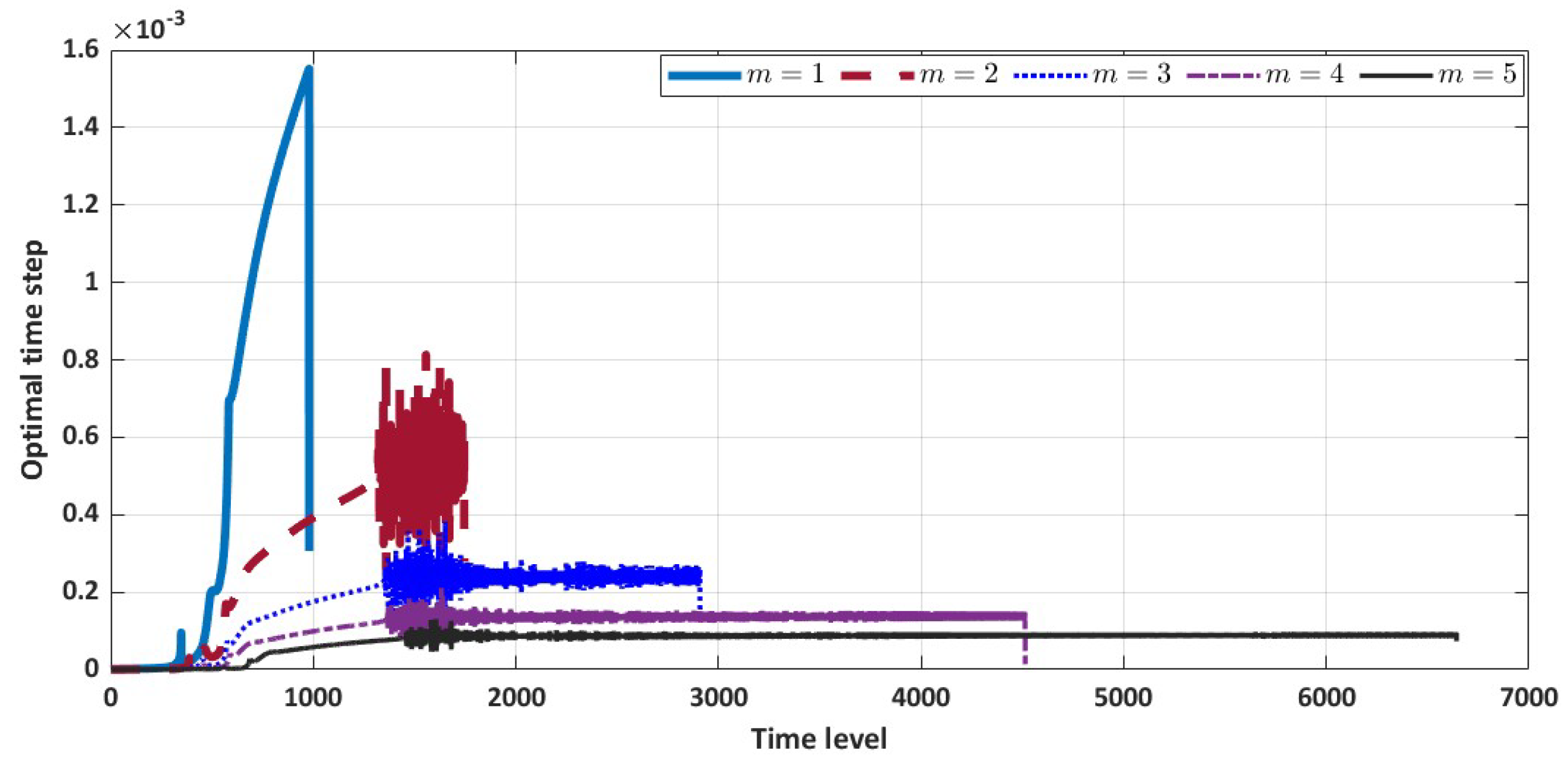
Next, we present the plot profile of the time step versus time level for each considered power term m. The plot is displayed in Figure 5. The optimal time step at each time level decreases substantially as the power term increases. This is expected because of the associated with the diffusive term. This power term m may impact the stability condition if a non-adaptive scheme is implemented.
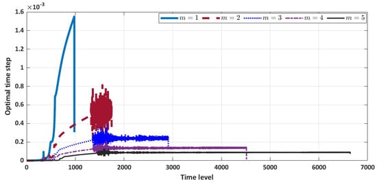
Figure 5.
Optimal time step for each time level with varying power m (, ).
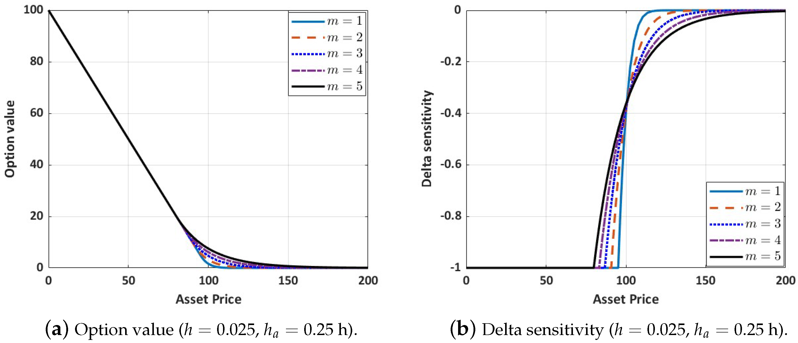
Finally, we display the plot profile and the numerical solutions of the option value and delta sensitivity for each power term m, as presented in Figure 6. For a fixed asset price, Figure 6 shows that the option value increases as the power term m increases. This is also reflected in the numerical solution presented in Table 16. Lee [7] describes that this feature given by the exotic options provides the buyer with the possibility of receiving a reasonably higher payoff than its vanilla counterpart. Moreover, in the money, the delta sensitivity decreases as the power term increases. Furthermore, out of the money, delta sensitivity increases as the power term increases. This is fully described in Table 17. Additionally, the numerical solution for gamma at some interpolated grid points is also listed in Table 18.
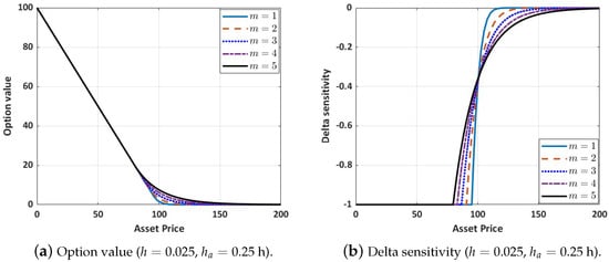
Figure 6.
Option value and delta sensitivity with varying power term m.

Table 16.
Option values with varying power term m (, ).

Table 17.
Delta sensitivity with varying power term m (, ).

Table 18.
Gamma with varying power term m (, ).
4. Conclusions
We have proposed a high-order adaptive numerical scheme for approximating a free boundary exotic power put options pricing problem on a non-uniform space grid for which a locally adopted mesh refinement strategy is implemented. Our proposed implementation leverages some advantages. By selecting time steps adaptively at each time level, we circumvent the stability challenges in an explicit time integration scheme, which could be more pronounced here due to the coefficient of the diffusive term. This is because the coefficient of the diffusive term involves , which can substantially vary and impact any stability criterion. However, the adaptive nature of our proposed method worked in our favor here. More importantly, by refining our space grid locally and allowing time steps to be adaptively selected based on regional variation and space grid distribution, the solution accuracy in the neighborhood of the left corner point, where large variation, discontinuity, and even singularity exist in the pricing model, was substantially improved.
The importance of our implementation can further be observed in the manner in which we recover highly accurate results with very coarse grids using the locally refined grid strategy at each time level. This gain will be very useful in a high-dimensional pricing model due to space complexity. We have already established in the numerical experiment that, even with a very coarse grid (), a reasonable solution accuracy was achieved with gamma when we concentrated more of the grid points in the locality of the left corner point.
In our future work, we hope to further extend our proposed method to include a suite of space grid stretching strategies and, possibly, a pure high-order adaptive space–time scheme for pricing free boundary Asian stochastic volatility models and other non-standard options. In the context of a pure high-order adaptive space–time scheme, the grid points in both the space and time grids will be dynamically selected and updated.
Author Contributions
Conceptualization, C.N. and W.D.; methodology, C.N.; software, C.N.; validation, C.N.; formal analysis, C.N.; investigation, C.N.; resources, C.N.; data curation, C.N.; writing—original draft preparation, C.N.; writing—review and editing, W.D.; visualization, C.N.; supervision, W.D.; project administration, W.D. All authors have read and agreed to the published version of the manuscript.
Funding
This research received no external funding.
Data Availability Statement
Not applicable.
Acknowledgments
The first author is funded in part by an NSERC Discovery Grant.
Conflicts of Interest
The authors declare no conflict of interest.
Code Availability
The MATLAB code for this work is freely available in GitHub through this link: https://github.com/Ifenonso/exotic/blob/main/Dormand_Prince_Refined_space_Adaptive_time_Exotic_Power_Options.m, (accessed on 8 June 2023).
References
- Dorm, J.R.; Prince, P.J. A family of embedded Runge-Kutta formulae. J. Comput. Appl. Math. 1980, 6, 19–26. [Google Scholar]
- Kim, J. Pricing of power options under the regime-switching model. J. Appl. Math. Inform. 2014, 32, 665–673. [Google Scholar] [CrossRef]
- Lee, Y.; Kim, Y.; Lee, J. Pricing various types of power options under stochastic volatility. Symmetry 2020, 12, 1911. [Google Scholar] [CrossRef]
- Topper, J. Finite element modeling of exotic options. In Operations Research Proceedings 1999; Springer: Berlin/Heidelberg, Germany, 2000; pp. 336–341. [Google Scholar]
- Heynen, R.C.; Kat, H.M. Pricing and hedging power options. Financ. Eng. Jpn. Mark. 1996, 3, 253–261. [Google Scholar] [CrossRef]
- Nwozo, C.R.; Fadugba, S.E. Mellin transform method for the valuation of some vanilla power options with non-dividend yield. Int. J. Pure Appl. Math. 2014, 96, 79–104. [Google Scholar] [CrossRef]
- Lee, J.K. A simple numerical method for pricing American power put options. Chaos Solitons Fractals 2020, 139, 110254. [Google Scholar] [CrossRef]
- Wang, J.Y.; Wang, C.J.; Dai, T.S.; Chen, T.C.; Liu, L.C.; Zhou, L. Efficient and robust combinatorial option pricing algorithms on the trinomial lattice for polynomial and barrier options. Math. Probl. Eng. 2022, 2022, 5843491. [Google Scholar] [CrossRef]
- Huang, C.S.; O’Hara, J.G.; Mataramvura, S. Highly efficient Shannon wavelet-based pricing of power options under the double exponential jump framework with stochastic jump intensity and volatility. Appl. Math. Comput. 2022, 414, 126669. [Google Scholar] [CrossRef]
- Okelola, M.O.; Govinder, K.S.; O’Hara, J.G. Solving a partial differential equation associated with the pricing of power options with time-dependent parameters. Math. Methods Appl. Sci. 2015, 38, 2901–2910. [Google Scholar] [CrossRef]
- Rao, B.P. Pricing geometric Asian power options under mixed fractional Brownian motion environment. Phys. A Stat. Mech. Its Appl. 2016, 446, 92–99. [Google Scholar]
- Esser, A. General valuation principles for arbitrary payoffs and applications to power options under stochastic volatility. Financ. Mark. Portf. Manag. 2003, 17, 351. [Google Scholar] [CrossRef]
- Kim, J.; Kim, B.; Moon, K.S.; Wee, I.S. Valuation of power options under Heston’s stochastic volatility model. J. Econ. Dyn. Control. 2012, 36, 1796–1813. [Google Scholar] [CrossRef]
- Blenman, L.P.; Bueno-Guerrero, A.; Clark, S.P. Pricing and hedging bond power exchange options in a stochastic string term-structure model. Risks 2022, 10, 188. [Google Scholar] [CrossRef]
- Ha, M.; Kim, D.; Ahn, S.; Yoon, J.H. The valuation of timer power options with stochastic volatility. J. Korean Soc. Ind. Appl. Math. 2022, 26, 296–309. [Google Scholar]
- Shukla, R.K.; Zhong, X. Derivation of high-order compact finite difference schemes for non-uniform grid using polynomial interpolation. J. Comput. Phys. 2005, 204, 404–429. [Google Scholar] [CrossRef]
- Shukla, R.K.; Tatineni, M.; Zhong, X. Very high-order compact finite difference schemes on non-uniform grids for incompressible Navier–Stokes equations. J. Comput. Phys. 2007, 224, 1064–1094. [Google Scholar] [CrossRef]
- Chen, Y.; Xiao, A.; Wang, W. An IMEX-BDF2 compact scheme for pricing options under regime-switching jump-diffusion models. Math. Methods Appl. Sci. 2019, 42, 2646–2663. [Google Scholar] [CrossRef]
- Lee, S.T.; Sun, H.W. Fourth-order compact scheme with local mesh refinement for option pricing in jump-diffusion model. Numer. Methods Partial. Differ. Equations 2012, 28, 1079–1098. [Google Scholar] [CrossRef]
- Zhao, J.; Corless, R.M. Compact finite difference method for integro-differential equations. Appl. Math. Comput. 2006, 177, 271–288. [Google Scholar] [CrossRef]
- Nwankwo, C.; Dai, W. An adaptive and explicit fourth order Runge–Kutta–Fehlberg method coupled with compact finite differencing for pricing American put options. Jpn. J. Ind. Appl. Math. 2021, 38, 921–946. [Google Scholar] [CrossRef]
- Abrahamsen, D.; Fornberg, B. Solving the Korteweg-de Vries equation with Hermite-based finite differences. Appl. Math. Comput. 2021, 401, 126101. [Google Scholar] [CrossRef]
- Dimitrov, Y.M.; Vulkov, L.G. High order finite difference schemes on non-uniform meshes for the time-fractional Black-Scholes equation. arXiv 2016, arXiv:1604.05178. [Google Scholar]
- Nwankwo, C.; Dai, W. On the efficiency of 5 (4) RK-embedded pairs with high order compact scheme and Robin boundary condition for options valuation. Jpn. J. Ind. Appl. Math. 2022, 39, 753–775. [Google Scholar] [CrossRef]
- Nwankwo, C.; Dai, W. Sixth-order compact differencing with staggered boundary schemes and 3 (2) Bogacki-Shampine pairs for pricing free-boundary options. arXiv 2022, arXiv:2207.14379. [Google Scholar]
- Bunch, D.S.; Johnson, H. The American put option and its critical stock price. J. Financ. 2000, 55, 2333–2356. [Google Scholar] [CrossRef]
- Gutiérrez, Ó. American option valuation using first-passage densities. Quant. Financ. 2013, 13, 1831–1843. [Google Scholar] [CrossRef]
- Tangman, D.Y.; Gopaul, A.; Bhuruth, M. A fast high-order finite difference algorithm for pricing American options. J. Comput. Appl. Math. 2008, 222, 17–29. [Google Scholar] [CrossRef]
- Leisen, D.P.; Reimer, M. Binomial models for option valuation-examining and improving convergence. Appl. Math. Financ. 1996, 3, 319–346. [Google Scholar] [CrossRef]
Disclaimer/Publisher’s Note: The statements, opinions and data contained in all publications are solely those of the individual author(s) and contributor(s) and not of MDPI and/or the editor(s). MDPI and/or the editor(s) disclaim responsibility for any injury to people or property resulting from any ideas, methods, instructions or products referred to in the content. |
© 2023 by the authors. Licensee MDPI, Basel, Switzerland. This article is an open access article distributed under the terms and conditions of the Creative Commons Attribution (CC BY) license (https://creativecommons.org/licenses/by/4.0/).

