Article

RPCGB Method for Large-Scale Global Optimization Problems

by
Abderrahmane Ettahiri
1,* and
Abdelkrim El Mouatasim
2
1
Laboratory LABSI, Faculty of Sciences Agadir (FSA), Ibnou Zohr University, B.P. 8106, Agadir 80000, Morocco
2
Department of Mathematics and Management, Faculty of Polydisciplinary Ouarzazate (FPO), Ibnou Zohr University, B.P. 284, Ouarzazate 45800, Morocco
*
Author to whom correspondence should be addressed.
Axioms 2023, 12(6), 603; https://doi.org/10.3390/axioms12060603
Submission received: 25 April 2023 / Revised: 15 June 2023 / Accepted: 16 June 2023 / Published: 18 June 2023

Abstract

:
In this paper, we propose a new approach for optimizing a large-scale non-convex differentiable function subject to linear equality constraints. The proposed method, RPCGB (random perturbation of the conditional gradient method with bisection algorithm), computes a search direction by the conditional gradient, and an optimal line search is found by a bisection algorithm, which results in a decrease of the cost function. The RPCGB method is designed to guarantee global convergence of the algorithm. An implementation and testing of the method are given, with numerical results of large-scale problems that demonstrate its efficiency.

1. Introduction

Non-convex optimization is a type of mathematical optimization problem in which the objective function to be optimized is not convex. Unlike convex optimization problems, non-convex problems can have multiple local optima, which can make it difficult to find the global optimum. Non-convex optimization has many applications in various fields, including finance (portfolio optimization, risk management, and option pricing) [1,2,3], computer vision (image segmentation, object recognition) [4,5], signal processing (compressed sensing, channel estimation, and equalization) [6,7,8], engineering (control systems, optimization of structures) [9,10], machine learning [11,12,13,14], and damage characterization [15] based on deep neural networks and the YUKI algorithm [16].
To solve non-convex optimization problems, two broad classes of techniques have been developed: deterministic and stochastic methods [17]. Deterministic methods include gradient-based methods, which rely on computing gradients of the objective function, and which can be sensitive to the choice of initialization and can converge to local optima. On the other hand, stochastic methods use randomness to explore the search space and can be less sensitive to initialization and more likely to find the global optimum.
Several reasons make stochastic methods more appropriate for non-convex optimization problems. Stochastic methods avoid getting stuck in local optima or saddle points, as they explore the search space more thoroughly. Additionally, complex non-convex optimization problems often have a large number of variables, making gradient-based methods computationally expensive. In contrast, stochastic methods can scale better to high-dimensional problems. Stochastic methods can also be more robust to noise and uncertainty in the problem formulation.
Scientific studies have shown the effectiveness of stochastic methods in solving non-convex optimization problems. One of the most widely studied deterministic methods that has been extended with random perturbations is gradient descent. For example, a study by Pogu and Souza de Cursi (1994) [18] compared the performance of deterministic gradient descent and stochastic gradient descent on a variety of non-convex optimization problems and found that stochastic gradient descent was more robust and could converge to better solutions. Another study by Mandt et al. (2016) [19] investigated the use of random perturbations in the context of Bayesian optimization and found that it could lead to better exploration of the search space and improved optimization performance. In addition to stochastic gradient descent, other deterministic methods have also been extended with random perturbations. For example, a study by Nesterov and Spokoiny (2017) [20] proposed a variant of the conjugate gradient method that adds random noise to the search direction at each iteration and showed that it could improve the convergence rate and solution quality compared to the standard conjugate gradient method. Another study by Songtao Lu et al. (2019) [21] proposed a variant of the projected gradient descent method that added random perturbations to the method, and they demonstrated its effectiveness in solving non-convex optimization problems.
We consider non-convex optimization problems with linear equality or inequality constraints of the form
m i n f ( x ) s . t A x b ν x μ
where f : R n R  is a continuously differentiable function, A is an m × n matrix with rank m, b is an m-vector, and the lower and upper bound vectors, ν and μ , may contain some infinite components; and
m i n f ( x ) s . t A x = b
where A R m × n , b R m , and f : R n R  is a continuously differentiable, non-convex objective function.
One possible numerical method to solve problem (1) is the conditional gradient with bisection (CGB) method. This method generates a sequence of feasible points { x t } t 0 , starting with an initial feasible point x 0 . A new feasible point x t + 1 is obtained from x t for each t > 0 , using an operator Q t (details can be found in Section 3). The iterations can be expressed as follows:
x t + 1 = Q t ( x t ) , t 0 .
In this paper, we present a new approach for solving large-scale non-convex optimization problems by using a modified version of the conditional gradient algorithm that incorporates stochastic perturbations. The main contribution of this paper is to propose the RPCGB algorithm, which is an extension of a method previously presented in [22] that was designed for small- and medium-scale problems. The RPCGB algorithm was developed to deal with large-scale global optimization problems and aims to determine the global optimum.
This method involves replacing the sequence of vectors { x t } t 0 with a sequence of random vectors { X t } t 0 , and the iterations are modified as follows:
X t + 1 = Q t ( X t ) + P t , t 0 ,
where P t is a random variable that is chosen appropriately, which is commonly known as the stochastic perturbation. It is important that the sequence { P t } t 0 converges to zero at a rate slow enough to avoid the sequence { X t } t 0 convergence to local minima. For more details, refer to Section 4.
The paper is structured as follows: Section 3 revisits the principle of the conditional gradient with bisection method, while Section 4 provides details on the random perturbation of the CGB method. Notations are introduced in Section 2, and in Section 5, the results of numerical experiments for non-convex optimization tests with linear constraints are presented for large-scale problems.

2. Notations and Assumptions

We denote by R the set of the real numbers, and E = R n is the n-dimensional real Euclidean space. x T denotes the transpose of x. We denote by x = x T x = ( x 1 2 + + x n 2 ) 1 / 2 the euclidean norm of x, and let
M = { x E | A x = b , x 0 }
and η * = min M f , the lower bound of f on M. Let us introduce
M φ = N φ M ; where N φ = { x E | f ( x ) φ } .
Supposing
φ > η * : m e a s ( M φ ) > 0 ,
φ > η * : M φ is not empty , closed , and bounded ,
f is continuously differentiable on E ,
where m e a s ( M φ ) is the measure of M φ .
As the space E is of finite dimensions, condition (3) holds true if M is bounded or if f is coercive, i.e., lim x + f ( x ) = + . Assumption (3) is satisfied when M comprises a series of neighborhoods of an optimal point x * that possesses a strictly positive measure, meaning x * can be approximated by a sequence of points from the interior of M.
We see that the results of assumptions (3) and (4) are
M = φ > η * N φ , i . e . , x M : φ > η * such that x M φ .
From (3) and (4), one has:
δ 1 = sup f ( x ) : x M φ < + .
Consequently, one deduces
δ 2 = sup d : x M φ < + ,
where d is the direction of conditional gradient method.
Thus,
ρ φ , ε = sup y ( x + α d ) : ( x , y ) M φ × M φ , 0 α ε < + ,
where α and ε are positive real numbers.

3. Conditional Gradient Method

3.1. Conditional Gradient Algorithm

The conditional gradient method, also known as the Frank–Wolfe algorithm, is an iterative optimization algorithm used to find the minimum of a convex function over a convex set. It was introduced by Philip Wolfe and Marguerite Frank in 1956 [23] and is one of the oldest nonlinear constrained optimization techniques. It has recently gained renewed interest due to its projection-free iterations and low memory requirement. This algorithm enables the approximation of a function during each iteration by utilizing the first-order Taylor series expansion.
The algorithm starts with an initial point in the feasible set and iteratively moves towards a direction that minimizes the gradient of the objective function over the feasible set. At each iteration, the algorithm solves a linear optimization problem over the feasible set to find the direction that minimizes the gradient.
The conditional gradient algorithm has several advantages over other optimization methods, including its ability to handle large-scale problems and its ability to find sparse solutions. However, it may converge slowly and may not always find the global minimum. Moving forward, we focus on a problem related to nonlinear programming that involves constraints in the form of linear equalities or inequalities of the form
minimize f ( x ) subject to x M
The search direction is d t : = s t x t , with s t being the optimal solution of a linear programming problem and
x t + 1 = Q t ( x k ) = x t + α k d t .
We ascertain the optimal step by selecting the value of α t that satisfies
f x t + α t d t = min 0 α 1 f x t + α d t .
The conditional gradient algorithm can be summarized as follows (Algorithm 1):
Algorithm 1 Conditional gradient algorithm.
1 Choose an initial point x ( 0 ) M in the feasible set M.
2: for t = 0 , 1 , 2 , , T do
3: Compute s t : = LMO M ( f ( x ( t ) ) ) : = arg min s M f ( x ( t ) ) s
                         ( LMO : Linear minimization oracle)
4: Let d t : = s t x ( t )                 (Conditional gradient direction)
5: Compute g t : = f ( x ( t ) ) , d t           (Conditional gradient gap)
6:  if   g t < ε then return   x ( t )
7: optimal line search step size
        α k arg min α [ 0 , 1 ] f ( x ( k ) + α d k )
8: Update x ( t + 1 ) : = x ( t ) + α k d t
9: end for
10: return x ( T )
For non-convex objectives, the conditional gradient algorithm may not converge to a global minimum, but it can still converge to a stationary point under certain conditions. Simon Lacoste-Julien and his colleagues have shown that the Frank–Wolfe algorithm can converge to a stationary point for non-convex objectives, as shown in [24].

3.2. Bisection Algorithm

In this paper, we employ the bisection algorithm to tackle the unconstrained optimization problem with one variable (8). The method is described in [25]. We refer to the recursive bisection procedure as bis  ( h , θ 1 , θ 2 , ϵ ) , which takes as inputs the h calculation procedure, the [ θ 1 , θ 2 ] interval, and the precision ϵ . The outputs of this procedure are an approximation of x m for the minimizer x * and h m for the minimum value of the h function over the [ θ 1 , θ 2 ] interval.
The recursive procedure iteration involves the application of the subsequent steps.
Step 0: If θ 2 θ 1 ϵ , go to step 1 , otherwise stop.
Step 1: Compute
θ 3 = θ 1 + θ 2 2 , θ 1 = θ 2 + θ 3 2 , θ 2 = θ 3 + θ 2 2 , h ( θ 3 ) , h θ 1 , h θ 2 .
Step 2: If h θ 1 h ( θ 3 ) h θ 2 , set θ 2 = θ 2 If h θ 1 h ( θ 3 ) h θ 2 , set θ 1 = θ 1 .
If h ( θ 3 ) min h θ 1 , h θ 2 , set θ 1 = θ 1 , θ 2 = θ 2 .
Step 3: Execute bis  ( h , θ 1 , θ 2 , ϵ ) with new inputs.

4. RPCGB Method

From [23], when it comes to objective functions that are non-convex, optimization algorithms based on gradients (CGB) cannot guarantee the discovery of the global minimum. Convex functions are the only ones for which CGB methods can find the global minimum. To deal with this issue, we suggest utilizing a suitable random perturbation method. Next, we will demonstrate how RPCGB can converge to a global minimum for non-convex optimization problems.
The sequence of real numbers x t t 0 is replaced by a sequence of random variables X t t 0 involving a random perturbation P t of the deterministic iteration (7). We have X 0 = x 0 ;
t 0 X t + 1 = Q t ( X t ) + P t = X t + α k d t + P t = X t + α t ( d t + P t α t ) ,
P t is independent from ( X t 1 , , X 0 ) , t 1 ,
where α t 0 satisfies Step 7 in the conditional gradient algorithm (Algorithm 1), and
X M Q t ( X ) + P t M .
Equation (9) can be considered a perturbation of the upward direction d t , which is substituted with a new direction D k = d t + P t α t . As a result, iterations (9) become:
X t + 1 = X t + α t D t .
In the literature [18,26,27], general properties can be found to select a sequence suitable for perturbation P t t 0 . Typically, perturbations that satisfy these features are produced using sequences of Gaussian laws.
We define a random vector Z t and use the symbols Φ t and ϕ t to represent its cumulative distribution function and probability density function, respectively.
The conditional probability density function of X t + 1 is represented by f t + 1 , and the conditional cumulative distribution function is designated as F t + 1 ( y | X t = x ) .
F t + 1 ( y | X t = x ) = P ( X t + 1 < y | X t = x ) .
We define a sequence of n-dimensional random vectors Z t t 0 M . Additionally, we also take into account ξ t t 0 , a decreasing sequence of positive real numbers that steadily approaches 0, where ξ 0 is less than or equal to 1.
Let P t = ξ t Z t
F t + 1 ( y | X t = x ) = P ( X t + 1 < y | X t = x ) .
It follows that
F t + 1 ( y | X t = x ) = P Z t < y Q t ( x ) ξ t = Φ t y Q t ( x ) ξ t .
Therefore, we have
f t + 1 ( y | X t = x ) = 1 ξ t n ϕ t y Q t ( x ) ξ t , y M .
Relation (5) shows that
y Q t ( x ) ρ ( φ , ε ) for ( x , y ) M φ × M φ .
We suppose that t h t ( t ) > 0 is a decreasing function defined on R + such that
y M φ ϕ t y Q t ( x ) ξ t h t ( ρ ( φ , ε ) ξ t ) .
For simplicity, let
Z t = 1 M ( Z t ) Z t ,
and Z N ( 0 , 1 ) , where Z is a random variable.
The procedure generates a sequence V t = f ( X t ) . By construction, this sequence is increasing and upper-bounded by η * .
t 0 : η * V t + 1 V t .
Thus, there exists V η * such that
V t V f o r t + .
Lemma 1.
Let P t = ξ t Z t and γ = f ( x 0 ) if Z t is given by (12). Then, there exists > 0 such that
P ( V t + 1 > ω | V t ω ) m e a s ( M γ M ω ) ξ t n h t ρ ( γ , ε ) ξ t > 0 ω ( η * , η * + ] ,
where n = dim ( E ) .
Proof. 
Let M ω = x M | f ( x ) < ω , for ω ( η * , η * + ] .
Since M φ M ^ ω , η * < φ < ω , it can be deduced from (2) that M ^ ω is non-empty and has a strictly positive measure.
If m e a s ( M M ^ ω ) = 0 for any ω ( η * , η * + ] , the result is immediate, since we have f ( x ) = η * on M .
Let us assume that there exists ε > 0 such that m e a s ( M M ^ ω ) > 0 . For ω ( η * , η * + ε ] , we have M ^ ω M ^ ε and m e a s ( M M ^ ω ) > 0 .
P ( X t M ^ ω ) = P ( X t S M ^ ω ) = M M ^ ω P ( X t d x ) > 0 for any ω ( η * , η * + ε ] and, since the sequence V i i 0 is increasing, we also have
X i i 0 M γ .
Thus
P ( X t M ^ ω ) = P ( X t N M ^ ω ) = M γ M ^ ω P ( X t d x ) > 0 for any ω ( η * , α * + ε ] .
Letting ω ( η * , α * + ε ] , we have from (13)
P ( V t + 1 > ω | V t ω ) = P ( X t + 1 M ^ ω | X i M ^ ω , i = 0 , , t ) .
However, the Markov chain produces
P ( X t + 1 M ^ ω | X i M ^ ω , i = 0 , , t ) = P ( X t + 1 M ^ ω | X t M ^ ω ) .
By the conditional probability rule,
P ( X t + 1 M ^ ω | X t M ^ ω ) = P ( X t + 1 M ^ ω , X t M ^ ω ) P ( X t M ^ ω ) .
Moreover,
P ( X t + 1 M ^ ω | X t M ^ ω ) = M M ^ ω P ( X t d x ) M ^ ω f t + 1 ( y | X t = x ) d y .
From (14), we have
P ( X t + 1 M ^ ω | X t M ^ ω ) = M γ M ^ ω P ( X t d x ) M ^ ω f t + 1 ( y | X t = x ) d y ,
and
P ( X t + 1 M ^ ω | X t M ^ ω ) inf x M γ M ^ ω M ^ ω f t + 1 ( y | X t = x ) d y M γ M ^ ω P ( X t d x ) .
Thus
P ( X t + 1 M ^ ω | X t M ^ ω ) inf x M γ M ^ ω M ^ ω f t + 1 ( y | X t = x ) d y .
Taking (10) into account, we have
P ( X t + 1 M ^ ω | X t M ^ ω ) 1 ξ t n inf x M γ M ^ ω M ^ ω ϕ t y Q t ( x ) ξ t d y .
Relation (5) shows that
y Q t ( x ) ρ ( γ , ε ) ,
and (11) yields
ϕ t y Q t ( x ) ξ t h t ρ ( γ , ε ) ξ t .
Hence,
P ( X t + 1 M ^ ω | X t M ^ ω ) 1 ξ t n inf x M γ M ^ ω M ^ ω h t ρ ( γ , ε ) ξ t d y .
P ( X t + 1 M ^ ω | X t M ^ ω ) m e a s ( M γ M ω ) ξ t n h t ρ ( γ , ε ) ξ t .
The following result, which follows from Borel–Catelli’s lemma (as described in [18], for example), is a consequence of the global convergence:
Lemma 2.
Let V t t 0 be a increasing sequence, upper-bounded by η * . Then, there exists V such that V t V for t + . Assume that there exists > 0 such that, for any ω ( α * , α * + ] , there is a sequence of strictly positive real numbers c t ( ω ) t 0 , such that
t 0 : P ( V t + 1 > ω | V t ω ) c t ( ω ) > 0 a n d t = 0 + c t ( ω ) = + .
Then V = η * almost surely.
Proof. 
For instance, see [18,28]. □
Theorem 1.
Assuming x 0 belongs to M, and letting γ = f ( x 0 ) , let the sequence ξ t be non-increasing, and
t = 0 + h t ρ ( γ , ε ) ξ t = + .
Then V = η * almost surely.
Proof. 
Let
c t ( ω ) = m e a s ( M γ M ω ) ξ t n h t ρ ( γ , ε ) ξ t > 0 .
Since the sequence ξ t t 0 is non increasing,
c t ( ω ) m e a s ( M γ M ω ) ξ t n h t ρ ( γ , ε ) ξ t > 0 .
Thus, Equation (15) shows that
t = 0 + c t ( ω ) m e a s ( M γ M ω ) ξ t n t = 0 + h t ρ ( γ , ε ) ξ t = + .
We can conclude that V = η * almost surely by applying Lemmas 1 and 2. □
Theorem 2.
Let Z t be defined by (12) and ξ t by
ξ t = b ^ log ( t + a ^ ) ,
where b ^ > 0 , a ^ > 0 , and t is the iteration number. If x 0 M , then for b ^ large enough, V = η * almost surely.
Proof. 
We have
ϕ t ( Z ) = 1 ( 2 π ) n exp ( 1 2 Z 2 ) = h t ( Z ) > 0 ,
so
h t ρ ( γ , ε ) ξ t = 1 ( 2 π ) n ( t + a ^ ) ρ ( γ , ε ) 2 / 2 b ^ .
For b ^ , such that
0 < ρ ( γ , ε ) 2 2 b ^ < 1 ,
we have
t = 0 + h t ρ ( γ , ε ) ξ t = + ;
furthermore, as per the previous Theorem 2, it can be deduced that V is almost surely equal to η * . □

5. Numerical Results

In this section, we present numerical results of six examples implemented using the CGB method and the perturbed RPCGB method. Our aim is to compare the performance of these two algorithms.
We begin by applying the algorithm to the initial value, which is X 0 = x 0 M . At each step t 0 , X t is known, and we calculate X t + 1 .
k sto denotes the number of perturbations. When k sto = 0 , the method used is the conditional gradient with bisection, without any perturbations (unperturbed conditional gradient with bisection method).
The Gaussian variates used in our experiments are generated using regular generator calls. Specifically, we use
ξ t = b ^ log ( t + 2 ) , where b ^ > 0 .
The definitions of the methods listed in the tables are as follows:
(i)
“CGB”, the method of conditional gradient and bisection;
(ii)
“RPCGB”, the method of random perturbation of conditional gradient and bisection.
The proposed RPCGB algorithm is implemented using the MATLAB programming language. We evaluate the performance of the RPCGB method and compare it with the CGB method for high-dimensional problems. We test the efficacy of these algorithms on several problems [29,30,31,32] with linear constraints, using predetermined feasible starting points x 0 . The results are presented in Table 1, Table 2, Table 3, Table 4, Table 5 and Table 6 and Figure 1, Figure 2, Figure 3, Figure 4, Figure 5 and Figure 6, where n denotes the dimension of the problem under consideration and n c represents the number of constraints. The reported test results include the optimal value f R P C G B * and the number of iterations k i t e r .
The optimal line search process of CGB and RPCGB is found using the bisection method with ϵ = 10 4 . We terminate the iterative process when either the best solution (global solution) is found or the maximum number of iterations has been reached.
All algorithms were run on a TOSHIBA Intel(R) Core(TM) CPU running at 2.40 GHz with 6 GB of RAM, a Core i7 processor, and the 64-bit Windows 7 Professional operating system. The “CPU” column in the table displays the mean CPU time for one run in seconds.
Problem 1.
The Neumaier 3 Problem (NF3) is a mathematical optimization problem introduced by Arnold Neumaier in 2003 (see [29]). The problem is defined as follows:
m i n i m i z e : j = 1 n ( x j 1 ) 2 j = 2 n x j x j 1 s u b j e c t t o : n 2 x j n 2 , j = 1 , , n
Problem 2.
The Cosine Mixture Problem (CM) is an optimization problem introduced by Breiman and Cutler in 1993 (see [29]). The problem is defined as follows:
m i n i m i z e : j = 1 n x j 2 0.1 j = 1 n cos ( 5 π x j ) s u b j e c t t o : 1 x j 1 , j = 1 , , n
Problem 3.
The Inverted Cosine Wave Function or the Cosine Mixture with Exponential Decay Problem. This is a commonly used benchmark problem in global optimization and was introduced by Price et al. in 2006 (see [30]). The problem is defined as follows:
m i n i m i z e : j = 1 n exp ( x j 2 x j + 1 2 0.5 x j x j + 1 8 ) cos ( 4 x j 2 + x j + 1 2 + 0.5 x j x j + 1 ) s u b j e c t t o : 5 x j 5 , j = 1 , , n
Problem 4.
The Epistatic Michalewicz Problem (EM) is a type of optimization problem commonly used as a benchmark in evolutionary computation and optimization. It was introduced by Michalewicz in 1996 (see [29]). The problem is defined as follows:
m i n i m i z e : j = 1 n sin ( y j ) ( sin ( j y j 2 π ) ) 20 s u b j e c t t o : 0 x j π , j = 1 , , n y j = x j cos ( π 6 ) x j + 1 sin ( π 6 ) , j = 1 , 3 , 5 , , n x j sin ( π 6 ) + x j + 1 cos ( π 6 ) , j = 2 , 4 , 6 , , n x j , j = n
Problem 5.
The problem is a mathematical optimization problem used in global optimization which comes from [32] and is defined as follows:
m i n i m i z e : j = 1 n ( x j 2 10 cos ( 2 π x j ) + 10 ) s u b j e c t t o : j = 1 n x j = 0 , 5.12 x j 5.12 , j = 1 , , n
Problem 6.
Rastrigin’s function is a non-convex, multi-modal function commonly used as a benchmark problem in optimization. It was introduced by Rastrigin in 1974 (see [31]) and is defined as:
m i n i m i z e : j = 1 n cos ( 2 π x j sin ( π 20 ) ) s u b j e c t t o : x j x j + 1 = 0.4 j = 1 , , n 1
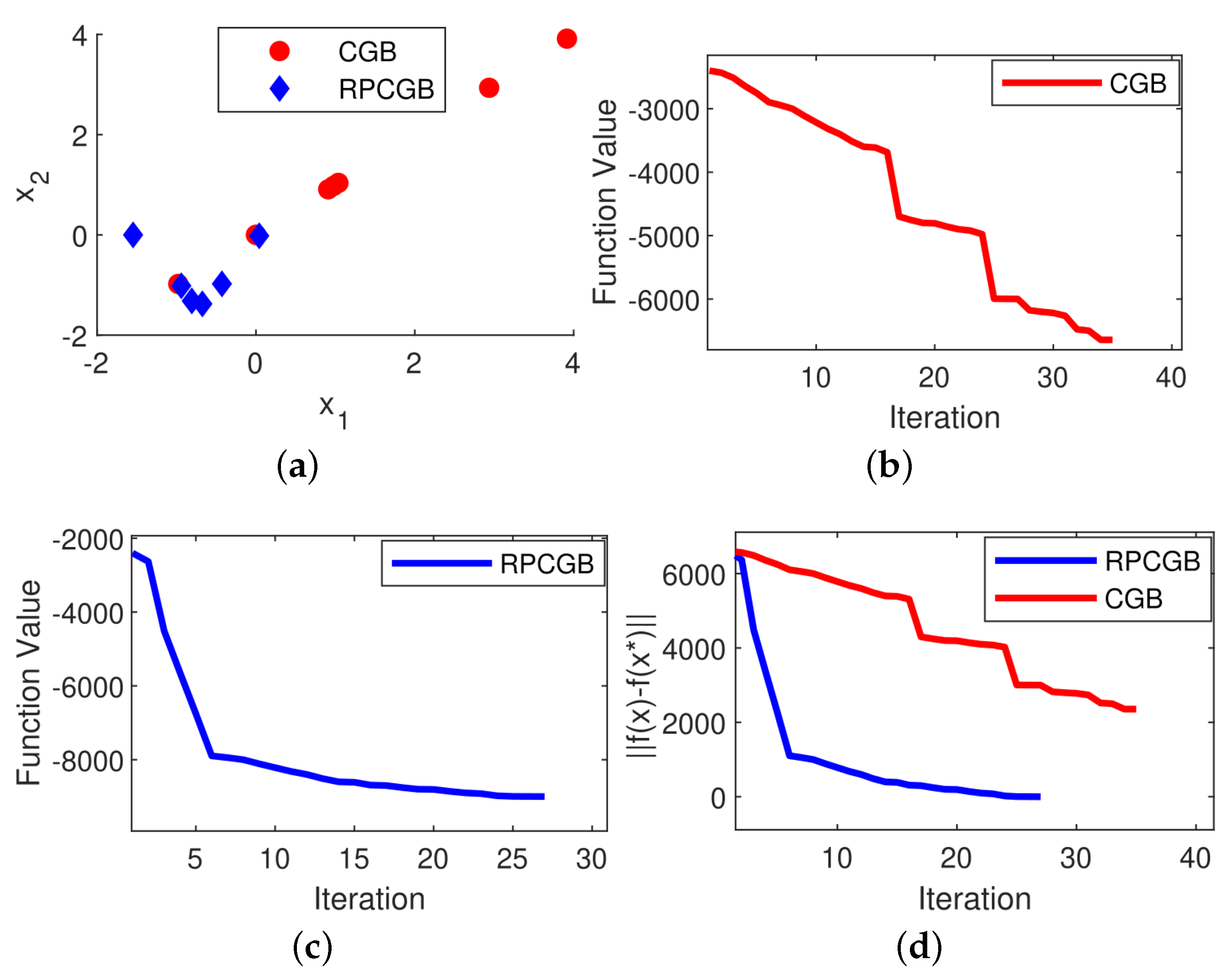
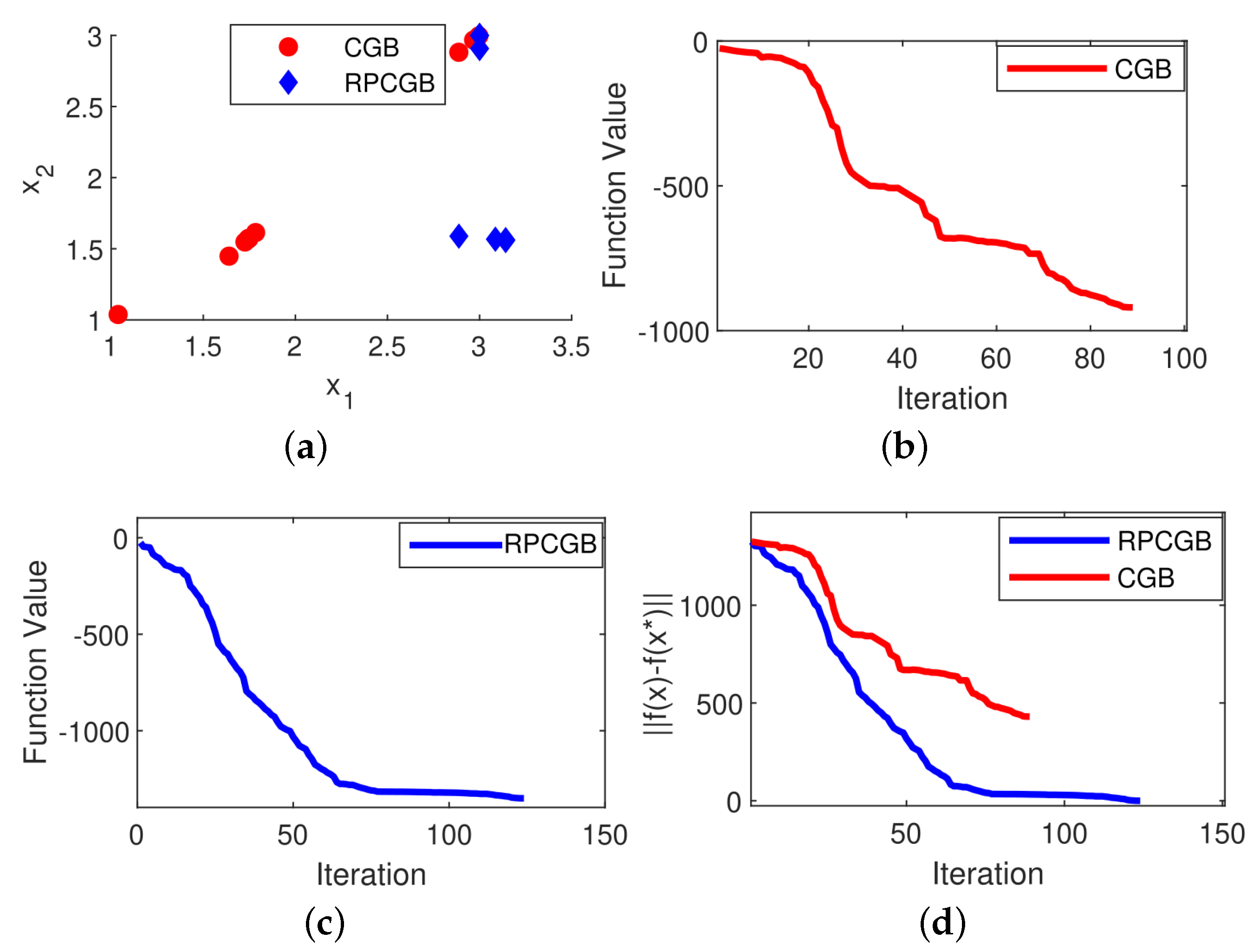
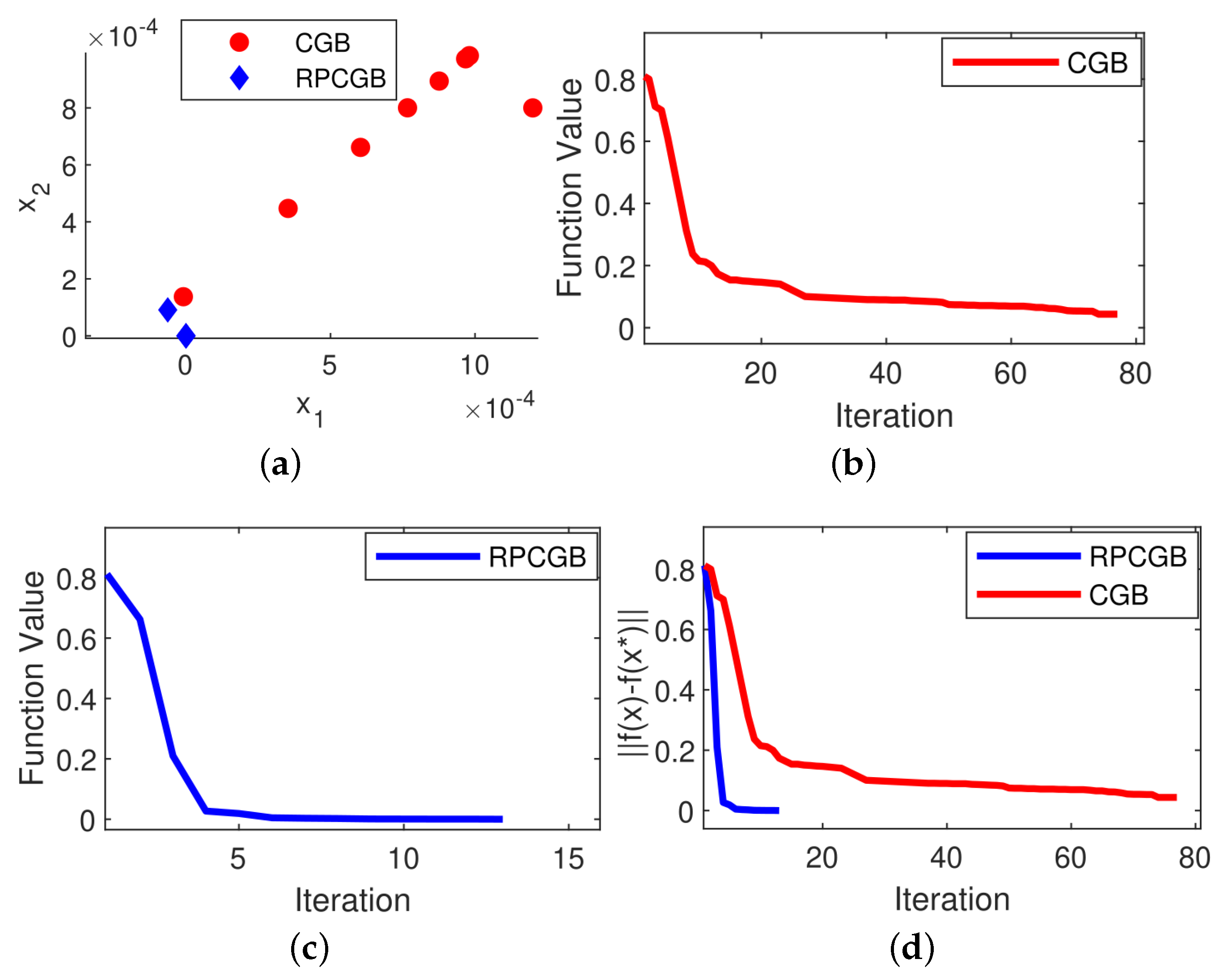
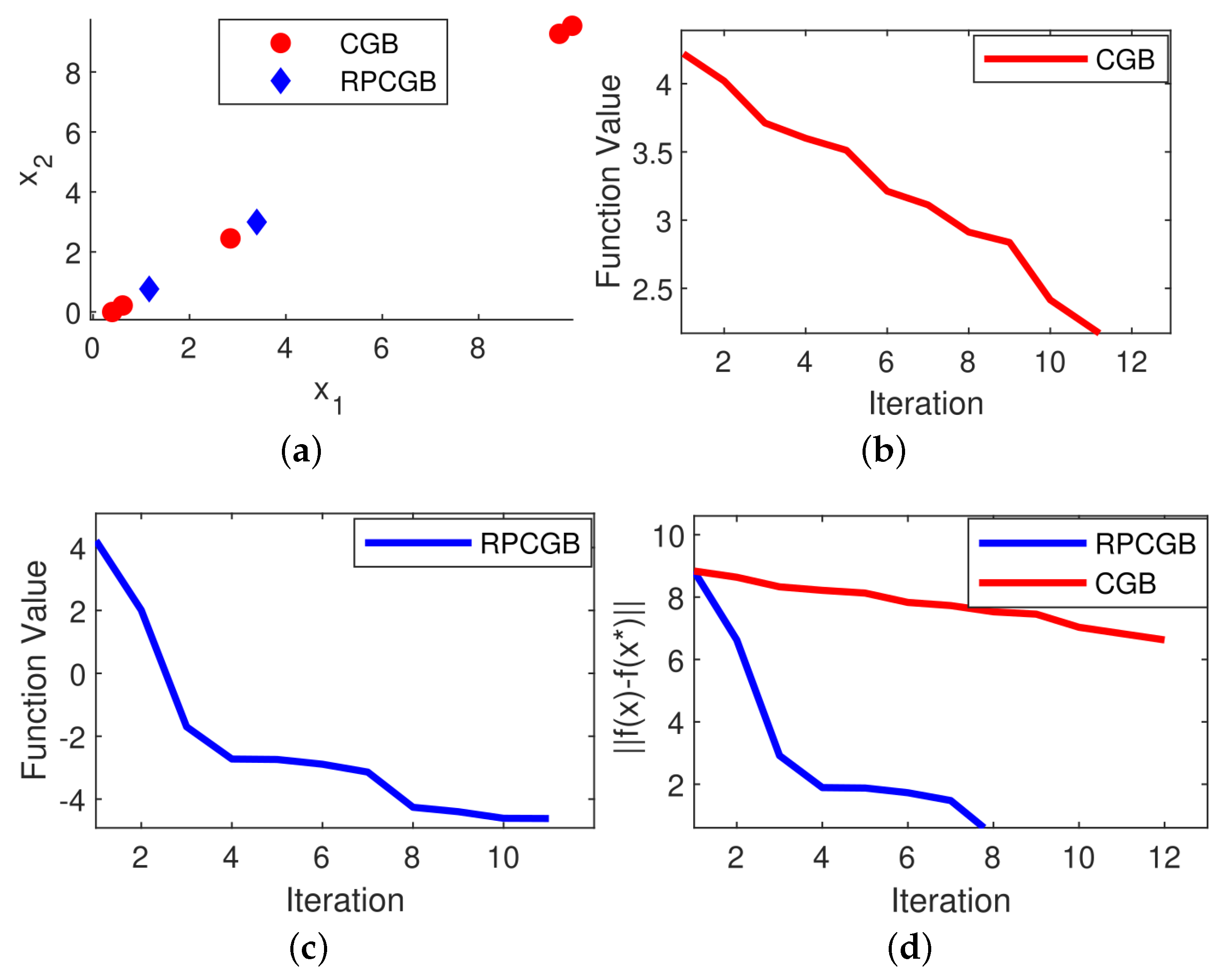
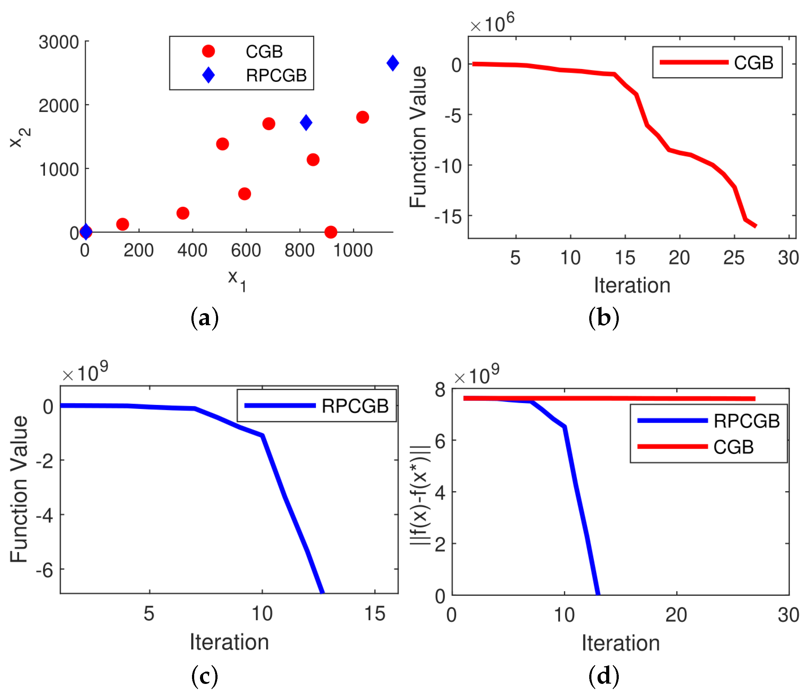
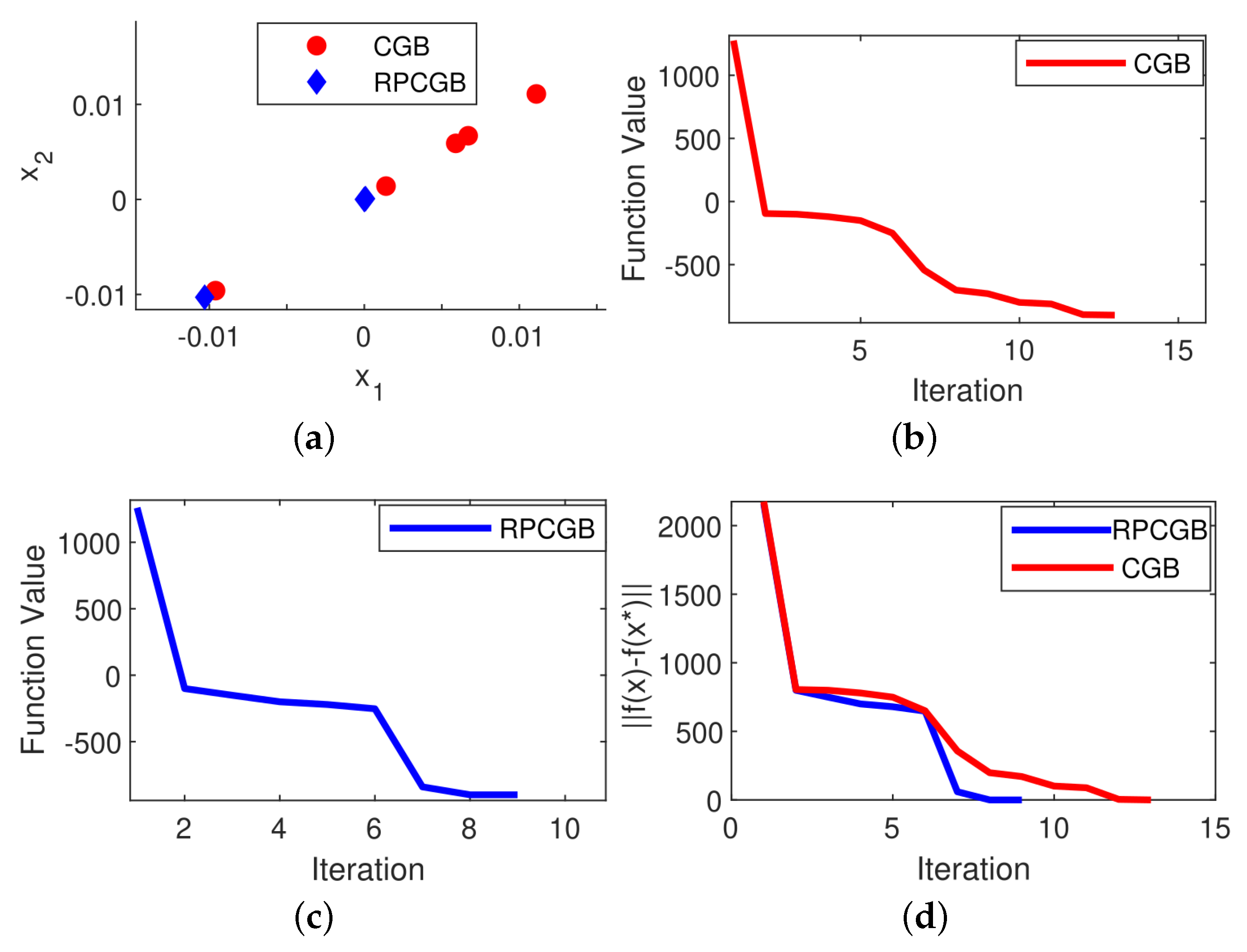
To gain a deeper understanding of the effect of the modifications on the proposed algorithm, we utilized a scatter plot that illustrates the distribution of the algorithm’s solutions in two dimensions for both the CGB and RPCGB algorithms. The goal was to generate scatter plots to depict the distribution of solutions in a 2D space for all problems when using two variables (n = 2). However, we found that for Problems 1 to 3, we were able to obtain the optimal solution value using only one iteration, which made the creation of a scatter plot unnecessary in this case. Thus, we generated a scatter plot of the solution distribution for the case of n = 900. This allowed us to effectively illustrate the distribution of solutions using scatter plots. In each algorithm, the scatter plot was generated at the first iteration and continued up to the limit of the required number of iterations to reach the solution. After analyzing Figure 1, Figure 2, Figure 3, Figure 4, Figure 5 and Figure 6, we concluded that the modified algorithm exhibited a more tightly clustered solution distribution in the scatter plot compared to the original algorithm.
We also present in Figure 1, Figure 2, Figure 3, Figure 4, Figure 5 and Figure 6 the results of plotting the objective function values in each iteration and the convergence performance for the CGB and RPCGB methods with 9000 variables. The plots (d) show that the proposed algorithm performs better than the CGB algorithm, with the majority of cases showing that the suggested algorithm achieves convergence in fewer iterations than the CGB algorithm. However, there is an exception observed in Problem 4, as presented in Figure 4, where the CGB algorithm stops early. This demonstrates that the convergence behavior of optimization algorithms can vary based on the problem being solved. It is worth noting that both algorithms terminated their execution before the 30th iteration, which is because a stopping criterion of approximately ϵ = 10 4 was met. The algorithms cease their iterations upon reaching the optimal solution (the local or global solution) or upon reaching the maximum number of iterations. We observe that the random perturbation has a significant effect on the convergence. This suggests that the changes made to the algorithm led to an improvement in its performance.
The results presented in Table 1, Table 2, Table 3, Table 4, Table 5 and Table 6 demonstrate that the CGB algorithm is capable of obtaining global solutions in certain instances regardless of the number of dimensions, such as Problem 2 (see Table 2). However, in some cases, the CGB algorithm fails to obtain global solutions as the number of dimensions increases, as seen in Problem 3 (see Table 3). In contrast, our RPCGB algorithm can obtain a global solution for all cases, and the computational results indicate that it performs effectively for these high-dimensional problems. These results also indicate that, for larger-dimensions problems, the CGB method necessitates a greater number of iterations to finalize the optimization process, whereas the RPCGB method does not, as evidenced by Problem 5. This difference can be explained by the k sto parameter, which denotes the number of perturbations. If the number of perturbations is raised, then the number of iterations needed to achieve the optimal solution is reduced.
When analyzing the obtained results, it is evident that the perturbed conditional gradient method with bisection algorithm (RPCGB) performs well compared to the conditional gradient algorithm (CGB).

6. Conclusions

In this work, we generalized the RPCGB method to solve large-scale non-convex optimization problems. The algorithms mentioned in this paper, specifically the conditional gradient algorithm, are commonly used optimization techniques for solving convex optimization problems. However, in the case of non-convex optimization problems, these algorithms may converge to a local minimum instead of the global minimum. To overcome this problem, the proposed approach introduces a random perturbation to the optimization problem. Specifically, at each iteration of the algorithm, a random perturbation is added to the Q t operator, which allows the algorithm to escape from local minima and explore the search space more effectively. The bisection algorithm is used to find the optimal step size along the search direction. It involves solving a one-dimensional optimization problem to find the step size that minimizes the objective function. By combining these two algorithms with the random perturbation approach, the proposed method is able to efficiently explore the search space for large-scale non-convex optimization problems under linear constraints and reach a global minimum. The tuning of the parameters k s t o and b ^ is related to the main difficulty in applying random perturbation in practice.
The RPCGB algorithm has the ability to solve various problems, such as control systems, as well as optimization problems in machine learning, robotics, and image reconstruction. There are problems that contain a part that is not smooth. Therefore, in the future, we plan to use the random perturbation of the conditional subgradient method with bisection algorithm to solve non-convex, non-smooth (non-differentiable) programming under linear constraints. Additionally, we intend to use the perturbed conditional gradient method to address non-convex optimization problems in support vector machines (SVM).
Author Contributions

Conceptualization, methodology, software, validation, formal analysis, investigation, writing—original draft preparation, writing—review and editing: A.E. and A.E.M. All authors have read and agreed to the published version of the manuscript.

Funding

This research received no external funding.

Data Availability Statement

Not applicable.

Acknowledgments

The authors would like to thank the referees for their fruitful suggestions, which helped us improve the quality of the paper.

Conflicts of Interest

The authors declare no conflict of interest.

References

  1. Frausto Solis, J.; Purata Aldaz, J.L.; González del Angel, M.; González Barbosa, J.; Castilla Valdez, G. SAIPO-TAIPO and Genetic Algorithms for Investment Portfolios. Axioms 2022, 42, 11. [Google Scholar] [CrossRef]
  2. Kuang, X.; Lamadrid, A.J.; Zuluaga, L.F. Pricing in non-convex markets with quadratic deliverability costs. Energy Econ. 2019, 80, 123–131. [Google Scholar] [CrossRef] [Green Version]
  3. Pang, L.P.; Chen, S.; Wang, J.H. Risk management in portfolio applications of non-convex stochastic programming. Appl. Math. Comput. 2015, 258, 565–575. [Google Scholar] [CrossRef]
  4. Chan, R.; Lanza, A.; Morigi, S.; Sgallari, F. Convex non-convex image segmentation. Numer. Math. 2018, 138, 635–680. [Google Scholar] [CrossRef]
  5. Oh, S.; Woo, H.; Yun, S.; Kang, M. Non-convex hybrid total variation for image denoising. J. Vis. Commun. Image Represent. 2013, 24, 332–344. [Google Scholar] [CrossRef]
  6. Chu, H.; Zheng, L.; Wang, X. Semi-blind millimeter-wave channel estimation using atomic norm minimization. IEEE Commun. 2018, 22, 2535–2538. [Google Scholar] [CrossRef]
  7. Di Martino, F.; Sessa, S. A Multilevel Fuzzy Transform Method for High Resolution Image Compression. Axioms 2022, 11, 551. [Google Scholar] [CrossRef]
  8. Wen, S.; Liu, G.; Chen, Q.; Qu, H.; Wang, Y.; Zhou, P. Optimization of precoded FTN signaling with MMSE-based turbo equalization. In Proceedings of the IEEE International Conference on Communications (ICC), Shanghai, China, 20–24 May 2019; pp. 1–6. [Google Scholar]
  9. Kaveh, A.; Hamedani, K.B. Improved arithmetic optimization algorithm and its application to discrete structural optimization. Structures 2022, 35, 748–764. [Google Scholar] [CrossRef]
  10. Zeng, G.Q.; Xie, X.Q.; Chen, M.R.; Weng, J. Adaptive population extremal optimization-based PID neural network for multivariable nonlinear control systems. Swarm Evolut. Comput. 2019, 44, 320–334. [Google Scholar] [CrossRef]
  11. El Mouatasim, A. Fast gradient descent algorithm for image classification with neural networks. Signal Image Video Process. 2020, 14, 1565–1572. [Google Scholar] [CrossRef]
  12. Nanuclef, R.; Frandi, E.; Sartori, C.; Allende, H. A novel Frank-Wolfe algorithm. Analysis and applications to large-scale SVM training. Inf. Sci. 2014, 285, 66–99. [Google Scholar] [CrossRef] [Green Version]
  13. Zheng, M.; Wang, F.; Hu, X.; Miao, Y.; Cao, H.; Tang, M. A Method for Analyzing the Performance Impact of Imbalanced Binary Data on Machine Learning Models. Axioms 2022, 11, 607. [Google Scholar] [CrossRef]
  14. Berrada, L.; Zisserman, A.; Kumar, M.P. Deep Frank-Wolfe for neural network optimization. In Proceedings of the International Conference on Learning Representations, New Orleans, LA, USA, 6–9 May 2019. [Google Scholar]
  15. Amoura, N.; Benaissa, B.; Al Ali, M.; Khatir, S. Deep Neural Network and YUKI Algorithm for Inner Damage Characterization Based on Elastic Boundary Displacement; Capozucca. Lect. Notes Civ. Eng. 2023, 317, 220–233. [Google Scholar]
  16. Benaissa, B.; Hocine, N.A.; Khatir, S.; Riahi, M.K.; Mirjalili, S. YUKI Algorithm and POD-RBF for Elastostatic and Dynamic Crack Identification. J. Comput. Sci. 2021, 55, 101451. [Google Scholar] [CrossRef]
  17. Moxnes, E. An Introduction to Deterministic and Stochastic Optimization, Analytical methods for Dynamic Modelers; MIT Press: Cambridge, MA, USA, 2015. [Google Scholar]
  18. Pogu, M.; Souza de Cursi, J.E. Global optimization by random perturbation of the gradient method with a fixed parameter. J. Glob. Optim. 1994, 5, 159–180. [Google Scholar] [CrossRef]
  19. Mandt, S.; Hoffman, M.; Blei, D. A variational analysis of stochastic gradient algorithms. In Proceedings of the 33rd International Conference on Machine Learning, New York, NY, USA, 19–24 June 2016; pp. 354–363. [Google Scholar]
  20. Nesterov, Y.; Spokoiny, V. Random gradient-free minimization of convex functions. Found. Comput. Math. 2017, 17, 527–566. [Google Scholar] [CrossRef]
  21. Lu, S.; Zhao, Z.; Huang, K.; Hong, M. Perturbed projected gradient descent converges to approximate second-order points for bound constrained nonconvex problems. In Proceedings of the IEEE International Conference on Acoustics, Speech and Signal Processing (ICASSP), Brighton, UK, 12–17 May 2019; pp. 5356–5360. [Google Scholar]
  22. El Mouatasim, A.; Ettahiri, A. Conditional gradient and bisection algorithms for non-convex optimization problem with random perturbation. Appl. Math. E-Notes 2022, 22, 142–159. [Google Scholar]
  23. Frank, M.; Wolfe, P. An Algorithm for Quadratic Programming. Naval Res. Logist. Q. 1956, 3, 95–110. [Google Scholar] [CrossRef]
  24. Khamaru, K.; Wainwright, M.J. Convergence guarantees for a class of non-convex and non-smooth optimization problems. J. Mach. Learn. Res. 2019, 20, 1–52. [Google Scholar]
  25. Baushev, A.N.; Morozova, E.Y. A multidimensional bisection method for minimizing function over simplex. Lect. Notes Eng. Comput. Sci. 2007, 2, 801–803. [Google Scholar]
  26. El Mouatasim, A.; Ellaia, R.; Souza de Cursi, J.E. Random perturbation of projected variable metric method for linear constraints nonconvex nonsmooth optimization. Int. J. Appl. Math. Comput. Sci. 2011, 21, 317–329. [Google Scholar]
  27. Bouhadi, M.; Ellaia, R.; Souza de Cursi, J.E. Random perturbations of the projected gradient for linearly constrained problems. Nonconvex Optim. Appl. 2001, 487–499. [Google Scholar]
  28. L’Ecuyer, P.; Touzin, R. On the Deng-Lin random number generators and related methods. Stat. Comput. 2003, 14, 5–9. [Google Scholar] [CrossRef] [Green Version]
  29. Ali, M.M.; Khompatraporn, C.; Zabinsky, Z.B. A numerical evaluation of several stochastic algorithms on selected continuous global optimization test problems. J. Glob. Optim. 2005, 31, 635–672. [Google Scholar] [CrossRef]
  30. Aslimani, N.; Ellaia, R. A new chaos optimization algorithm based on symmetrization and levelling approaches for global optimization. Numer. Algorithms 2018, 79, 1021–1047. [Google Scholar] [CrossRef]
  31. Che, H.; Li, C.; He, X.; Huang, T. An intelligent method of swarm neural networks forequalities constrained nonconvex optimization. Neurocomputing 2015, 167, 569–577. [Google Scholar] [CrossRef]
  32. Li, C.; Li, D. An extension of the Fletcher Reeves method to linear equality constrained optimization problem. Appl. Math. Comput. 2003, 219, 10909–10914. [Google Scholar] [CrossRef]
Figure 1. (a) Scatter plot of solution distribution for the CGB and RPCGB algorithms (n = 900). (b) Objective function values over iterations for the CGB method (n = 9000). (c) Objective function values over iterations for the RPCGB method (n = 9000). (d) Convergence performance for the CGB and RPCGB methods with n = 9000 for Problem 1.
Axioms 12 00603 g001
Figure 2. (a) Scatter plot of solution distribution for the CGB and RPCGB algorithms (n = 900). (b) Objective function values over iterations for the CGB method (n = 9000). (c) Objective function values over iterations for the RPCGB method (n = 9000). (d) Convergence performance for the CGB and RPCGB methods with n = 9000 for Problem 2.
Axioms 12 00603 g002
Figure 3. (a) Scatter plot of solution distribution for the CGB and RPCGB algorithms (n = 900). (b) Objective function values over iterations for the CGB method (n = 9000). (c) Objective function values over iterations for the RPCGB method (n = 9000). (d) Convergence performance for the CGB and RPCGB methods with n = 9000 for Problem 3.
Axioms 12 00603 g003
Figure 4. (a) Scatter plot of solution distribution for the CGB and RPCGB algorithms (n = 2). (b) Objective function values over iterations for the CGB method (n = 9000). (c) Objective function values over iterations for the RPCGB method (n = 9000). (d) Convergence performance for the CGB and RPCGB methods with n = 9000 for Problem 4.
Axioms 12 00603 g004
Figure 5. (a) Scatter plot of solution distribution for the CGB and RPCGB algorithms (n = 2). (b) Objective function values over iterations for the CGB method (n = 9000). (c) Objective function values over iterations for the RPCGB method (n = 9000). (d) Convergence performance for the CGB and RPCGB methods with n = 9000 for Problem 5.
Axioms 12 00603 g005
Figure 6. (a) Scatter plot of solution distribution for the CGB and RPCGB algorithms (n = 2). (b) Objective function values over iterations for the CGB method (n = 4000). (c) Objective function values over iterations for the RPCGB method (n = 4000). (d) Convergence performance for the CGB and RPCGB methods with n = 4000 for Problem 6.
Axioms 12 00603 g006
Table 1. The results obtained from the CGB and RPCGB algorithms.
Problem 1Algorithm
CGBRPCGB
n n c k iter CPU f CGB * k iter CPU k sto f RPCGB *
500100090.11−1.06 ×  10 6 90.682−1.61 ×  10 7
900180090.13−3.41 ×  10 6 40.252−6.32 ×  10 7
20004000103.27−1.08 ×  10 7 65.315−3.53 ×  10 8
400080001219.33−5.53 ×  10 7 727.2710−1.48 ×  10 9
600012,0001935.70−1.34 ×  10 7 946.5410−3.35 ×  10 9
900018,0002787.92−1.61 ×  10 7 1391.1610−7.62 ×  10 9
Table 2. The results obtained from the CGB and RPCGB algorithms.
Problem 2Algorithm
CGBRPCGB
n n c k iter CPU f CGB * k iter CPU k sto f RPCGB *
500100040.07−5020.021−50
900180050.09−9020.051−90
2000400070.11−199.9930.091−200
4000800090.19−40040.121−400
600012,000100.37−599.9970.151−600
900018,000130.42−90090.211−900
Table 3. The results obtained from the CGB and RPCGB algorithms.
Problem 3Algorithm
CGBRPCGB
n n c k iter CPU f CGB * k iter CPU k sto f RPCGB *
500100050.05−498.9930.041−499
900180070.07−898.9960.071−898.76
20004000110.12−1475.44110.191−1998.99
40008000180.31−2951.62120.471−3999
600012,000240.79−4427.81190.741−5998.87
900018,000351.03−6642.08270.961−8998.25
Table 4. The results obtained from the CGB and RPCGB algorithms.
Problem 4Algorithm
CGBRPCGB
n n c k iter CPU f CGB * k iter CPU k sto f RPCGB *
50010002311.41−131.814519.5325−176.72
90018002917.06−214.795721.3430−293.51
200040003442.66−417.956971.2630−536.38
400080005667.18−768.227596.0250−1.06 ×  10 3
600012,0007379.63−846.0194110.6370−1.11 ×  10 3
900018,0008999.25−919.85124136.7190−1.35 ×  10 3
Table 5. The results obtained from the CGB and RPCGB algorithms.
Problem 5Algorithm
CGBRPCGB
n n c k iter CPU f CGB * k iter CPU k sto f RPCGB *
500500198.044.71 ×  10 4 149.23701.38 ×  10 11
9009002914.138.51 ×  10 4 1414.25703.05 ×  10 10
200020004233.090.00972645.311504.96 ×  10 10
400040003053.630.01941797.272007.93 ×  10 7
600060005971.470.029119122.543007.93 ×  10 9
900090007792.550.043613153.168007.93 ×  10 5
Table 6. The results obtained from the CGB and RPCGB algorithms.
Problem 6Algorithm
CGBRPCGB
n n c k iter CPU f CGB * k iter CPU k sto f RPCGB *
50049920.09−1.885650.2810−4.0147
900899191.650.703370.3810−4.4432
1000999130.920.1626121.0810−4.6572
20001999211.702.0535817.2440−3.1399
30002999232.960.9158927.5460−3.2145
40003999121.472.00971148.56100−4.6168
Disclaimer/Publisher’s Note: The statements, opinions and data contained in all publications are solely those of the individual author(s) and contributor(s) and not of MDPI and/or the editor(s). MDPI and/or the editor(s) disclaim responsibility for any injury to people or property resulting from any ideas, methods, instructions or products referred to in the content.