Article

Study on the Nonlinear Dynamics of the (3+1)-Dimensional Jimbo-Miwa Equation in Plasma Physics

1
School of Electronics and Information, Guangdong Polytechnic Normal University, Guangzhou 510665, China
2
School of Physics and Electronic Information Engineering, Henan Polytechnic University, Jiaozuo 454003, China
*
Author to whom correspondence should be addressed.
Axioms 2023, 12(6), 592; https://doi.org/10.3390/axioms12060592
Submission received: 24 May 2023 / Revised: 8 June 2023 / Accepted: 13 June 2023 / Published: 15 June 2023
(This article belongs to the Special Issue Special Topics in Differential Equations with Applications)

Abstract

:
The Jimbo-Miwa equation (JME) that describes certain interesting (3+1)-dimensional waves in plasma physics is studied in this work. The Hirota bilinear equation is developed via the Cole-Hopf transform. Then, the symbolic computation, together with the ansatz function schemes, are utilized to seek exact solutions. Some new solutions, such as the multi-wave complexiton solution (MWCS), multi-wave solution (MWS) and periodic lump solution (PLS), are successfully constructed. Additionally, different types of travelling wave solutions (TWS), including the dark, bright-dark and singular periodic wave solutions, are disclosed by employing the sub-equation method. Finally, the physical characteristics and interaction behaviors of the extracted solutions are depicted graphically by assigning appropriate parameters. The obtained outcomes in this paper are more general and newer. Additionally, they reveal that the used methods are concise, direct, and can be employed to study other partial differential equations (PDEs) in physics.

1. Introduction

Complex phenomena in engineering and physics can usually be reduced to PDEs [1,2,3,4,5,6]. The study on the properties of these equations such as the explicit analytical solutions, especially the soliton solutions, is of great significance since they can help us to better understand complex phenomena and their inner nature. Up to now, a series of different effective methods have been developed to construct the exact solutions of PDEs such as the Hirota bilinear method [7,8,9,10], Wang’s Bäcklund transformation-based method [11,12], trial equation method [13,14], Sardar subequation method [15,16,17], exp-function method [18,19], Riccati equation mapping method [20] and so on [21,22,23,24,25,26,27,28]. In this work, we aim to examine the (3+1)-dimensional JME given by [29]:
Π x x x y + 3 Π x Π x y + 3 Π y Π x x + 2 Π y t 3 Π x z = 0 ,
Equation (1) is derived from the second equation in the well-known KP hierarchy of integrable systems and used widely to describe some interesting (3+1)-dimensional waves in plasma and optics. Up to now, some important research achievements have been developed to deal with Equation (1). In [29], the Kudryashov method is used with the symbolic computation and different solutions are obtained. In [30], four kinds of different wave forms are constructed via the Hirota bilinear method. In [31], the authors employ the direct algebraic method to handle Equation (1) and some different wave forms are constructed. In [32], several closed-form solutions are developed by using the singular manifold method. In [33], the Riccati equation mapping method is adopted. The exp-function method is utilized in [34] and some generalized solutions with parameters are constructed. In [35], the authors carry out the linear superposition principle to seek for multi-resonant solutions of Equation (1). In [36], the authors make use of the generalized Bernoulli equation method to inquire into Equation (1). In this study, we will present th results of a detailed investigation of Equation (1). The rest of the content of this work is given as follows. In Section 2, the Cole-Hopf transform is adopted to establish the Hirota bilinear form, and symbolic computation, combined with the ansatz function schemes, is utilized to search for the MWCS, MWS and PLS. In Section 3, the sub-equation method is used to seek for the TWSs. In Section 4, the physical characteristics and interaction behaviors are presented. Finally, we reach a conclusion in Section 5.

2. The Hirota Bilinear Equation and the Exact Solutions

To obtain the Hirota bilinear form of Equation (1), we adopt the Cole-Hopf transform as:
Π = 2 ln ( Ξ ) x ,
Taking it into Equation (1), we can obtain the bilinear form as:
( D x 3 D y + 2 D y D t 3 D x D z ) Ξ Ξ = 0 .
Here, the definition of the operators D x m D τ n is [37,38]:
D x m D t n f g = ( 𝜕 𝜕 x 𝜕 𝜕 x ) m ( 𝜕 𝜕 t 𝜕 𝜕 t ) n f ( x , t ) g ( x , t ) | x = x , t = t .
Additionally, there are
D x ( f g ) = f x g f g x ,
D x 2 ( f g ) = f x x g 2 f x g x + f g x x ,
D x 2 ( f f ) = 2 ( f x x f f x 2 ) ,
D t D x ( f g ) = f t x g f t g x f x g t + g t x f .

2.1. The MWCS

In order to find the MWCS, it is assumed that the solution of Equation (3) is:
Ξ = u 1 e p + u 2 e p + u 3 sin ( q ) + u 4 sin h ( ρ ) ,
with
{ p = x + k 1 y + k 2 z + k 3 t q = x + k 4 y + k 5 z + k 6 t ρ = x + k 7 y + k 8 z + k 9 t ,
where u i ( i = 1 , 2 , 3 , 4 . ) and k i ( i = 1 , 2 , 3 , 4 , 5 , 6 , 7 , 8 , 9 . ) are constants that can be determined later. Substituting Equation (5) into Equation (3) and setting the coefficients of different terms to zero, an algebraic equation system is attained. Solving it, we derive:
Case 1:
k 1 = 3 k 2 2 ( k 9 + 2 ) ,   k 2 = k 2 ,   k 3 = k 9 ,   k 4 = 3 k 2 2 ( k 9 + 2 ) ,   k 5 = k 2 k 2 k 9 2 + k 9 ,   k 6 = k 9 + 1 ,   k 7 = 3 k 2 2 ( 2 + k 9 ) ,   k 8 = k 2 ,   k 9 = k 9 ,   u 1 = u 1 ,   u 2 = u 2 ,   u 3 = u 3 ,   u 4 = u 4 .
The MWCS is obtained as:
Π ( x , y , z , t ) = 2 [ u 1 e x + 3 k 2 2 ( k 9 + 2 ) y + k 2 z + k 9 t u 2 e ( x + 3 k 2 2 ( k 9 + 2 ) y + k 2 z + k 9 t ) + u 3 cos ( x 3 k 2 2 ( k 9 + 2 ) y + k 2 k 2 k 9 2 + k 9 z + ( k 9 + 1 ) t ) + u 4 cos h ( x + 3 k 2 2 ( 2 + k 9 ) y + k 2 z + k 9 t ) ] u 1 e x + 3 k 2 2 ( k 9 + 2 ) y + k 2 z + k 9 t + u 2 e ( x + 3 k 2 2 ( k 9 + 2 ) y + k 2 z + k 9 t ) + u 3 sin ( x 3 k 2 2 ( k 9 + 2 ) y + k 2 k 2 k 9 2 + k 9 z + ( k 9 + 1 ) t ) + u 4 sin h ( x + 3 k 2 2 ( 2 + k 9 ) y + k 2 z + k 9 t ) .
For the special case u 1 = u 2 = 2 u 4 , Equation (6) becomes:
Case 2:
k 1 = k 1 ,   k 2 = k 2 ,   k 3 = 2 + 3 k 2 2 k 1 ,   k 4 = k 1 ,   k 5 = 2 k 1 k 2 ,   k 6 = 1 + 3 k 2 2 k 1 ,   k 7 = k 1 ,   k 8 = k 2 ,   k 9 = 2 + 3 k 2 2 k 1 ,   u 1 = u 1 ,   u 2 = u 2 ,   u 3 = u 3 ,   u 4 = u 4 .
Thus, we can obtain the MWCS as:
Π ( x , y , z , t ) = 2 [ u 1 e x + k 1 y + k 2 z + ( 2 + 3 k 2 2 k 1 ) t u 2 e ( x + k 1 y + k 2 z + ( 2 + 3 k 2 2 k 1 ) t ) + u 3 cos ( x k 1 y + ( 2 k 1 k 2 ) z + ( 1 + 3 k 2 2 k 1 ) t ) + u 4 cos h ( x + k 1 y + k 2 z + ( 2 + 3 k 2 2 k 1 ) t ) ] u 1 e x + k 1 y + k 2 z + ( 2 + 3 k 2 2 k 1 ) t + u 2 e ( x + k 1 y + k 2 z + ( 2 + 3 k 2 2 k 1 ) t ) + u 3 sin ( x k 1 y + ( 2 k 1 k 2 ) z + ( 1 + 3 k 2 2 k 1 ) t ) + u 4 sin h ( x + k 1 y + k 2 z + ( 2 + 3 k 2 2 k 1 ) t ) .
Case 3:
k 1 = k 1 ,   k 2 = 2 3 ( 2 k 1 + k 1 k 9 ) ,   k 3 = k 9 ,   k 4 = k 1 ,   k 5 = 2 3 ( k 1 + k 1 k 9 ) ,   k 6 = 1 + k 9 ,   k 7 = k 1 ,   k 8 = 2 3 ( 2 k 1 + k 1 k 9 ) ,   k 9 = k 9 ,   u 1 = u 1 ,   u 2 = u 2 ,   u 3 = u 3 ,   u 4 = u 4 .
Thus, we obtain the MWCS solution as:
Π ( x , y , z , t ) = 2 [ u 1 e x + k 1 y + 2 3 ( 2 k 1 + k 1 k 9 ) z + k 3 t u 2 e ( x + k 1 y + 2 3 ( 2 k 1 + k 1 k 9 ) z + k 3 t ) + u 3 cos ( x + k 4 y + k 5 z + ( k 9 1 ) t ) + u 4 cos h ( x + k 1 y + 2 3 ( 2 k 1 + k 1 k 9 ) z + k 9 t ) ] u 1 e x + k 1 y + 2 3 ( 2 k 1 + k 1 k 9 ) z + k 3 t + u 2 e ( x + k 1 y + 2 3 ( 2 k 1 + k 1 k 9 ) z + k 3 t ) + u 3 sin ( x + k 4 y + k 5 z + ( k 9 1 ) t ) + u 4 sin h ( x + k 1 y + 2 3 ( 2 k 1 + k 1 k 9 ) z + k 9 t ) .
Case 4:
k 1 = 3 k 5 2 ( k 9 1 ) ,   k 2 = 2 k 5 ( 1 + k 9 ) k 9 1 ,   k 3 = k 9 ,   k 4 = 3 k 5 2 ( k 9 1 ) ,   k 5 = k 5 ,   k 6 = k 9 1 ,   k 7 = 3 k 5 2 ( k 9 1 ) ,   k 8 = 2 k 5 ( 1 + k 9 ) k 9 1 ,   k 9 = k 9 ,   u 1 = u 1 ,   u 2 = u 2 ,   u 3 = u 3 ,   u 4 = u 4 .
Accordingly, the MWCS is:
Π ( x , y , z , t ) = 2 [ u 1 e x 3 k 5 2 ( k 9 1 ) y 2 k 5 ( 1 + k 9 ) k 9 1 z + k 9 t u 2 e ( x 3 k 5 2 ( k 9 1 ) y 2 k 5 ( 1 + k 9 ) k 9 1 z + k 9 t ) + u 3 cos ( x + 3 k 5 2 ( k 9 1 ) y + k 5 z + ( k 9 1 ) t ) + u 4 cos h ( x 3 k 5 2 ( k 9 1 ) y 2 k 5 ( 1 + k 9 ) k 9 1 z + k 9 t ) ] u 1 e x 3 k 5 2 ( k 9 1 ) y 2 k 5 ( 1 + k 9 ) k 9 1 z + k 9 t + u 2 e ( x 3 k 5 2 ( k 9 1 ) y 2 k 5 ( 1 + k 9 ) k 9 1 z + k 9 t ) + u 3 sin ( x + 3 k 5 2 ( k 9 1 ) y + k 5 z + ( k 9 1 ) t ) + u 4 sin h ( x 3 k 5 2 ( k 9 1 ) y 2 k 5 ( 1 + k 9 ) k 9 1 z + k 9 t ) .
Case 5:
k 1 = k 4 ,   k 2 = k 8 ,   k 3 = ( 2 + 3 k 8 2 k 4 ) ,   k 4 = k 4 ,   k 5 = ( 2 k 4 + k 8 ) ,   k 6 = ( 1 + 3 k 8 2 k 4 ) ,   k 7 = k 4 ,   k 8 = k 8 ,   k 9 = ( 2 + 3 k 8 2 k 4 ) ,   u 1 = u 1 ,   u 2 = u 2 ,   u 3 = u 3 ,   u 4 = u 4 .
where k 4 0 . Thus, we can obtain the MWCS as:
Π ( x , y , z , t ) = 2 [ u 1 e x k 4 y + k 8 z ( 2 + 3 k 8 2 k 4 ) t u 2 e ( x k 4 y + k 8 z ( 2 + 3 k 8 2 k 4 ) t ) + u 3 cos ( x + k 4 y ( 2 k 4 + k 8 ) z ( 1 + 3 k 8 2 k 4 ) t ) + u 4 cos h ( x k 4 y + k 8 z ( 2 + 3 k 8 2 k 4 ) t ) ] u 1 e x k 4 y + k 8 z ( 2 + 3 k 8 2 k 4 ) t + u 2 e ( x k 4 y + k 8 z ( 2 + 3 k 8 2 k 4 ) t ) + u 3 sin ( x + k 4 y ( 2 k 4 + k 8 ) z ( 1 + 3 k 8 2 k 4 ) t ) + u 4 sin h ( x k 4 y + k 8 z ( 2 + 3 k 8 2 k 4 ) t ) .
For the special case u 1 = u 2 = 2 u 4 , Equations (6)–(10) become:
Π ( x , y , z , t ) = 2 cot ( x 3 k 2 2 ( k 9 + 2 ) y + k 2 k 2 k 9 2 + k 9 z + ( k 9 + 1 ) t ) .
Π ( x , y , z , t ) = 2 cot ( x k 1 y + ( 2 k 1 k 2 ) z + ( 1 + 3 k 2 2 k 1 ) t ) .
Π ( x , y , z , t ) = 2 cot ( x + k 4 y + k 5 z + ( k 9 1 ) t ) .
Π ( x , y , z , t ) = 2 cot ( x + 3 k 5 2 ( k 9 1 ) y + k 5 z + ( k 9 1 ) t ) .
Π ( x , y , z , t ) = 2 cot ( x + k 4 y ( 2 k 4 + k 8 ) z ( 1 + 3 k 8 2 k 4 ) t ) .

2.2. The MWS

Here, we can use the following ansatz function:
Ξ = u 1 cos ( p ) + u 2 cos h ( q ) + u 3 cos h ( ρ ) ,
with
{ p = x + k 1 y + k 2 z + k 3 t q = x + k 4 y + k 5 z + k 6 t ρ = x + k 7 y + k 8 z + k 9 t ,
where u i ( i = 1 , 2 , 3 . ) and k i ( i = 1 , 2 , 3 , 4 , 5 , 6 , 7 , 8 , 9 . ) are constants that can be determined later. In the same manner, substituting Equation (11) into Equation (3) and making the corresponding adjustments, we derive:
Case 1:
k 1 = k 1 ,   k 2 = k 2 ,   k 3 = 2 + 3 k 2 2 k 1 ,   k 7 = k 1 ,   k 8 = 2 k 1 k 2 ,   k 9 = 1 + 3 k 2 2 k 1 ,   u 1 = u 1 ,   u 2 = 0 ,   u 3 = u 3 .
Then, we obtain the MWS as:
Π ( x , y , z , t ) = 2 [ u 1 sin ( x + k 1 y + k 2 z + ( 2 + 3 k 2 2 k 1 ) t ) + u 3 sin h ( x k 1 y ( 2 k 1 + k 2 ) z + ( 1 + 3 k 2 2 k 1 ) t ) ] u 1 cos ( x + k 1 y + k 2 z + ( 2 + 3 k 2 2 k 1 ) t ) + u 3 cos h ( x k 1 y ( 2 k 1 + k 2 ) z + ( 1 + 3 k 2 2 k 1 ) t ) .
Case 2:
k 1 = k 1 ,   k 2 = 2 k 1 k 5 ,   k 3 = 1 3 k 5 2 k 1 ,   k 4 = k 1 ,   k 5 = k 5 ,   k 6 = 2 3 k 5 2 k 1 ,   u 1 = u 1 ,   u 2 = u 2 ,   u 3 = 0 .
Thus, we obtain the MWS as:
Π ( x , y , z , t ) = 2 [ u 1 sin ( x + k 1 y ( 2 k 1 + k 5 ) z ( 1 + 3 k 5 2 k 1 ) t ) + u 2 sin h ( x k 1 y + k 5 z ( 2 + 3 k 5 2 k 1 ) t ) ] u 1 cos ( x + k 1 y ( 2 k 1 + k 5 ) z ( 1 + 3 k 5 2 k 1 ) t ) + u 2 cos h ( x k 1 y + k 5 z ( 2 + 3 k 5 2 k 1 ) t ) .

2.3. The PLS

The solution of Equation (3) is assumed as:
Ξ = u 1 sin ( p ) + u 2 cos h ( q ) + k 7 ,
with
{ p = x + k 1 y + k 2 z + k 3 t q = x + k 4 y + k 5 z + k 6 t ,
where u i ( i = 1 , 2 . ) and k i ( i = 1 , 2 , 3 , 4 , 5 , 6 , 7 . ) are constants to be determined later. In the same manner, substituting Equation (14) into Equation (3) and making the corresponding adjustments, we derive:
Case 1:
k 1 = k 1 ,   k 2 = 2 3 k 1 ( k 6 1 ) ,   k 3 = k 6 + 1 ,   k 4 = k 1 ,   k 5 = 2 3 k 1 ( 2 + k 6 ) ,   k 6 = k 6 ,   k 7 = 0 ,   u 1 = u 1 , u 2 = u 2 .
The PLS to Equation (1) is:
Π ( x , y , z , t ) = 2 [ u 1 cos ( x + k 1 y + 2 3 k 1 ( k 6 1 ) z + ( k 6 + 1 ) t ) + u 2 sin h ( x k 1 y 2 3 k 1 ( 2 + k 6 ) z + k 6 t ) ] u 1 sin ( x + k 1 y + 2 3 k 1 ( k 6 1 ) z + ( k 6 + 1 ) t ) + u 2 cos h ( x k 1 y 2 3 k 1 ( 2 + k 6 ) z + k 6 t ) .
Case 2:
k 1 = 3 k 2 2 ( k 6 1 ) ,   k 2 = k 2 ,   k 3 = k 6 + 1 ,   k 4 = 3 k 2 2 ( k 6 1 ) ,   k 5 = 2 k 2 ( k 6 + 1 ) k 6 1 ,   k 6 = k 6 ,   k 7 = 0 ,   u 1 = u 1 ,   u 2 = u 2 .
Thus, we obtain the PLS of Equation (1) as:
Π ( x , y , z , t ) = 2 [ u 1 cos ( x + 3 k 2 2 ( k 6 1 ) y + k 2 z + ( k 6 + 1 ) t ) + u 2 sin h ( x 3 k 2 2 ( k 6 1 ) y 2 k 2 ( k 6 + 1 ) k 6 1 z + k 6 t ) ] u 1 sin ( x + 3 k 2 2 ( k 6 1 ) y + k 2 z + ( k 6 + 1 ) t ) + u 2 cos h ( x 3 k 2 2 ( k 6 1 ) y 2 k 2 ( k 6 + 1 ) k 6 1 z + k 6 t ) .
Case 3:
k 1 = 3 k 5 2 ( k 3 + 1 ) ,   k 2 = k 5 ( 2 k 3 ) k 3 + 1 ,   k 3 = k 3 ,   k 4 = 3 k 5 2 ( k 3 + 1 ) ,   k 5 = k 5 ,   k 6 = k 3 1 ,   k 7 = 0 ,   u 1 = u 1 ,   u 2 = u 2
The PLS of Equation (1) is obtained as:
Π ( x , y , z , t ) = 2 [ u 1 cos ( x 3 k 5 2 ( k 3 + 1 ) y + k 5 ( 2 k 3 ) k 3 + 1 z + k 3 t ) + u 2 sin h ( x + 3 k 5 2 ( k 3 + 1 ) y + k 5 z + ( k 3 1 ) t ) ] u 1 sin ( x 3 k 5 2 ( k 3 + 1 ) y + k 5 ( 2 k 3 ) k 3 + 1 z + k 3 t ) + u 2 cos h ( x + 3 k 5 2 ( k 3 + 1 ) y + k 5 z + ( k 3 1 ) t ) .
Case 4:
k 1 = k 4 ,   k 2 = 2 3 k 4 ( k 3 2 ) ,   k 3 = k 3 ,   k 4 = k 4 ,   k 5 = 2 3 k 4 ( k 3 + 1 ) ,   k 6 = k 3 1 ,   k 7 = 0 ,   u 1 = u 1 ,   u 2 = u 2 .
Thus, the PLS of Equation (1) is attained as:
Π ( x , y , z , t ) = 2 [ u 1 cos ( x k 4 y 2 3 k 4 ( k 3 2 ) z + k 3 t ) + u 2 sin h ( x + k 4 y + 2 3 k 4 ( k 3 + 1 ) z + ( k 3 1 ) t ) ] u 1 sin ( x k 4 y 2 3 k 4 ( k 3 2 ) z + k 3 t ) + u 2 cos h ( x + k 4 y + 2 3 k 4 ( k 3 + 1 ) z + ( k 3 1 ) t ) .
Case 5:
k 1 = k 1 ,   k 2 = k 2 ,   k 3 = 2 + 3 k 2 2 k 1 ,   k 4 = k 1 ,   k 5 = 2 k 1 k 2 ,   k 6 = 1 + 3 k 2 2 k 1 ,   k 7 = 0 ,   u 1 = u 1 ,   u 2 = u 2 .
We obtain the PLS of Equation (1) as:
Π ( x , y , z , t ) = 2 [ u 1 cos ( x + k 1 y + k 2 z + ( 2 + 3 k 2 2 k 1 ) t ) + u 2 sin h ( x k 1 y ( 2 k 1 + k 2 ) z + ( 1 + 3 k 2 2 k 1 ) t ) ] u 1 sin ( x + k 1 y + k 2 z + ( 2 + 3 k 2 2 k 1 ) t ) + u 2 cos h ( x k 1 y ( 2 k 1 + k 2 ) z + ( 1 + 3 k 2 2 k 1 ) t ) .

3. The TWS

This section aims to study the TWS using the sub-equation method [39,40]. For this end, we apply the following variable transformation to Equation (1):
Π ( x , y , z , t ) = ( χ ) ,   χ = m x + n y + k z + s t ,
where m, n, k, and s are non-zero constants. Equation (1) can be converted as:
m 3 n ( 4 ) + 6 m 2 n + ( 2 n s 3 m k ) = 0 ,
where ( 4 ) = d 4 d χ 4 , = d 2 d χ 2 , = d d χ . Integrating Equation (21) with respect to χ once and setting the integral constant to zero, we derive:
m 3 n + 3 m 2 n ( ) 2 + ( 2 n s 3 m k ) = 0 .
Based on the sub-equation method, the solution of Equation (22) can be assumed as:
( χ ) = i = 0 c ε i i ( χ ) .
where ε i ( i = 0 , 1 , 2 , , c . ) are constants that can be determined later. Additionally, there is:
( χ ) = σ + 2 ( χ ) .
Here, σ is a constant. Equation (24) has the following different solutions:
( χ ) = { σ tan h ( σ χ ) , σ < 0 σ cot h ( σ χ ) , σ < 0 σ tan ( σ χ ) , σ > 0 σ cot ( σ χ ) , σ > 0 1 ζ + Λ , Λ is a constant , σ = 0 .
We can determine the value of c in Equation (23) via balancing and ( ) 2 in Equation (22) as:
c = 1 .
Then, Equation (23) becomes:
( χ ) = ε 0 + ε 1 ( χ ) .
Substituting Equation (27) with Equation (24) into Equation (22) and setting their coefficients of the different powers of ( χ ) to zero, it yields:
Solving them, we derive:
0 ( χ ) : 3 k m σ ε 1 + 2 n s σ ε 1 + 2 m 3 n σ 2 ε 1 + 3 m 2 n σ 2 ε 1 2 = 0 , 2 ( χ ) : 3 k m ε 1 n s ε 1 + 8 m 3 n σ ε 1 + 6 m 2 n σ ε 1 2 = 0 , 4 ( χ ) :   6 m 3 n ε 1 + 3 m 2 n ε 1 2 = 0 .
Case 1:
ε 0 = ε 0 ,   ε 1 = ε 1 ,   m = ε 1 2 ,   n = n ,   k = k ,   s = ε 1 ( 3 k + n σ ε 1 2 ) 4 n ,   σ = σ .
Thus, the TWS of Equation (1) can be obtained as:
Π ( x , y , z , t ) = ε 0 ε 1 σ tan h [ σ ( ε 1 2 x + n y + k z ε 1 ( 3 k + n σ ε 1 2 ) 4 n t ) ] , σ < 0 .
Π ( x , y , z , t ) = ε 0 ε 1 σ cot h [ σ ( ε 1 2 x + n y + k z ε 1 ( 3 k + n σ ε 1 2 ) 4 n t ) ] , σ < 0 .
Π ( x , y , z , t ) = ε 0 + ε 1 σ tan [ σ ( ε 1 2 x + n y + k z ε 1 ( 3 k + n σ ε 1 2 ) 4 n t ) ] , σ > 0 .
Π ( x , y , z , t ) = ε 0 ε 1 σ cot [ σ ( α 1 2 x + n y + k z ε 1 ( 3 k + n σ ε 1 2 ) 4 n t ) ] ,   σ > 0 .
Case 2:
ε 0 = ε 0 ,   ε 1 = 2 m ,   m = m ,   n = n ,   k = 2 ( 2 m 3 n σ n s ) 3 m ,   s = s ,   σ = σ .
Thus, the TWS of Equation (1) can be obtained as:
Π ( x , y , z , t ) = ε 0 + 2 m σ tan h [ σ ( m x + n y 2 ( 2 m 3 n σ n s ) 3 m z + s t ) ] , σ < 0 .
Π ( x , y , z , t ) = α 0 + 2 m σ cot h [ σ ( m x + n y 2 ( 2 m 3 n σ n s ) 3 m z + s t ) ] , σ < 0 .
Π ( x , y , z , t ) = ε 0 2 m σ tan [ σ ( m x + n y 2 ( 2 m 3 n σ n s ) 3 m z + s t ) ] , σ > 0 .
Π ( x , y , z , t ) = ε 0 + 2 m σ cot [ σ ( m x + n y 2 ( 2 m 3 n σ n s ) 3 m z + s t ) ] ,   σ > 0 .

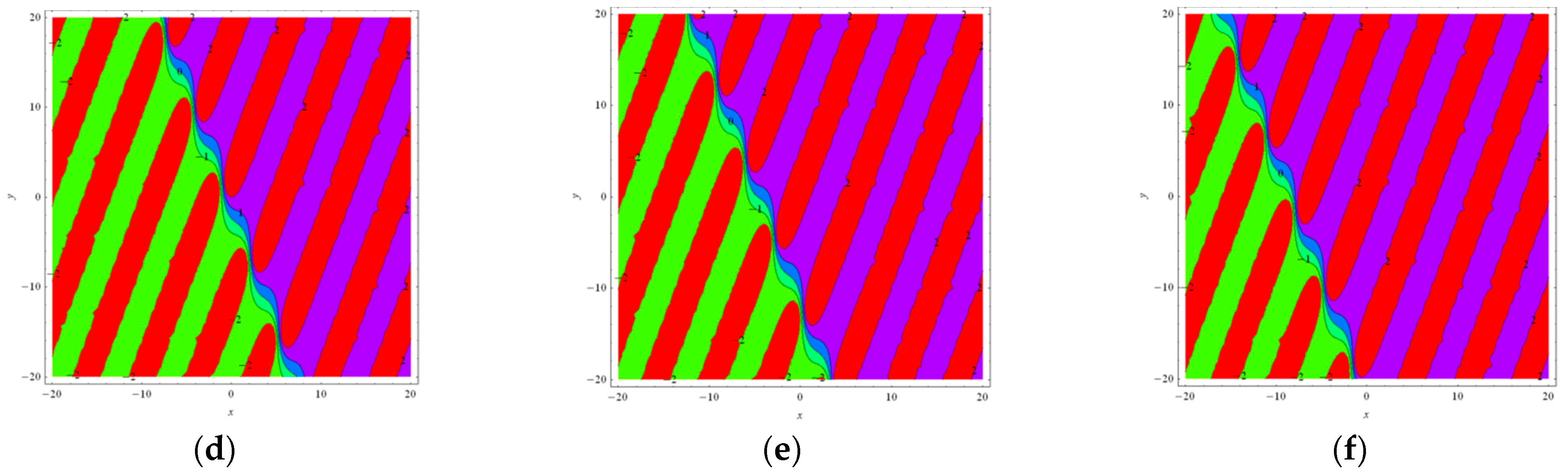
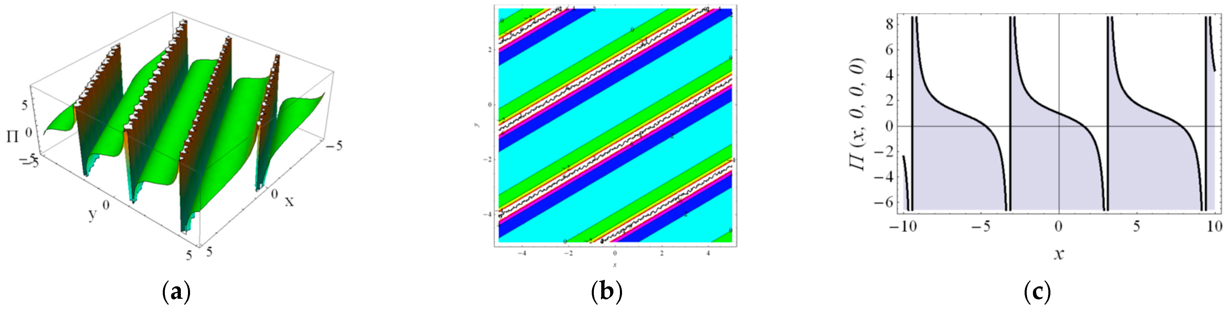
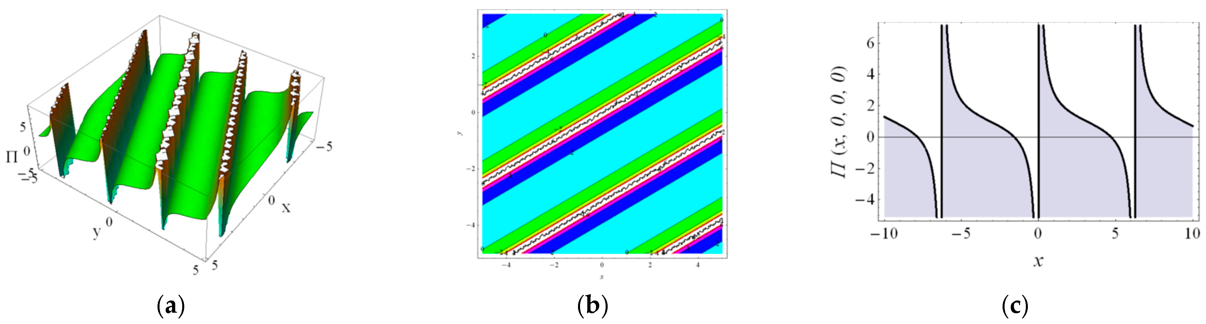
4. The Physical Interpretations

The obtained solutions will be presented by the 3D plot and 2D contour in this section by taking the reasonable parameters.
By assigning the parameters as k 2 = 1 , k 9 = 2 , u 1 = 1 , u 2 = 1 , u 3 = 1 , the multi-wave complexiton solution given by Equation (6) for the different time is illustrated in Figure 1 in the form of the 3D plot and 2D contour. Obviously, we can find there is a collision phenomenon between the singular periodic wave and the lump in the outline. As t increases, the waveform propagates in the negative direction of the x axis and y axis.
We illustrate the dynamic behavior of Equation (12) by selecting k 1 = 1 , k 2 = 1 , u 1 = 0.6 , u 2 = 0.4 in Figure 2. From this, collision phenomena between the breather waves and singular periodic waves are revealed. We can observe that the waveform travels along the negative direction of the x axis and positive direction of y axis.
Selecting k 1 = 1 , k 2 = 2 , u 1 = 1 , u 2 = 1 , u 3 = 1 , u 4 = 1 , we present the performance of Equation (15) in Figure 3. Here, it can be found the waveform propagates along the negative direction of the x axis and positive direction of y axis. Additionally, the outline of the wave can be explained as the interaction between lump solution and trigonometric function solution.
By using the parameters as ε 0 = 1 , ε 1 = 1 , n = 1 , k = 1 , σ = 1 , the dynamic characteristics of Equation (28) are revealed in Figure 4, where Figure 4a is the 3D plot, Figure 4b is the 2D contour and Figure 4c represents the 2D curve. In our observation, it is a dark wave. With the same parameters, Figure 5 illustrates the behaviors of Equations (3) and (10), which is a bright-dark wave.
The performances of Equations (29) and (30) are presented in Figure 6 and Figure 7, respectively with ε 0 = 1 , ε 1 = 1 , n = 1 , k = 1 , σ = 1 . We find that the profiles are both singular periodic waves.

5. Conclusions and Future Recommendation

In this article, we obtained multi-wave complexiton solutions, multi-wave solutions and periodic lump solutions of the (3+1)-dimensional Jimbo-Miwa equation with the help of the Hirota bilinear method. Besides, we also construct its diverse travelling wave solutions like the dark, bright-dark and singular periodic wave solutions by applying the sub-equation method. The evolution phenomenon of these different solutions are described graphically. From these descriptions, the physical behavior and the interaction are presented. The obtained results in this work are all new and have not been reported elsewhere. Additionally, they show that the methods adopted are effective and direct, and can moreover be used to study the other PDEs arising in physics.
In recent years, the interest in fractal and fractional calculus [41,42,43,44,45,46,47,48,49] has intensified in different fields due to their strong ability to describe complex phenomena. Applying the fractal and fractional calculus to Equation (1) and obtaining the exact solutions will animate our future research.

Author Contributions

Conceptualization, K.-J.W.; methodology, K.-J.W.; writing—original draft preparation, B.-Q.Z.; supervision, K.-J.W.; writing—review and editing, P.X.; data curation, H.H. All authors have read and agreed to the published version of the manuscript.

Funding

This work was supported by Guangzhou Basic Research Program (Grant No. 202201011286), Scientific Research Startup Project of Guangdong Polytechnic Normal University (Grant No. 2021SDKYA032).

Data Availability Statement

The data that support the findings of this study are available from the corresponding author upon reasonable request.

Conflicts of Interest

This research does not have any conflicts of interest.

Nomenclature

Multi-wave complexiton solutions MWCS
Multi-wave solutionsMWS
Periodic lump solutionsPLS
Travelling wave solutionsTWS
The Jimbo-Miwa equationJME
Travelling wave solutionsTWS

References

  1. Sohail, M.; Nazir, U.; Bazighifan, O.; El-Nabulsi, R.A.; Selim, M.M.; Alrabaiah, H.; Thounthong, P. Significant involvement of double diffusion theories on viscoelastic fluid comprising variable thermophysical properties. Micromachines 2021, 12, 951. [Google Scholar] [CrossRef]
  2. Nazir, U.; Saleem, S.; Al-Zubaidi, A.; Shahzadi, I.; Feroz, N. Thermal and mass species transportation in tri-hybridized Sisko martial with heat source over vertical heated cylinder. Int. Commun. Heat Mass Transf. 2022, 134, 106003. [Google Scholar] [CrossRef]
  3. Wang, K.J.; Si, J. Dynamic properties of the attachment oscillator arising in the nanophysics. Open Phys. 2023, 21, 20220214. [Google Scholar] [CrossRef]
  4. Lü, X.; Chen, S.-J. New general interaction solutions to the KPI equation via an optional decoupling condition approach. Commun. Nonlinear Sci. Numer. Simul. 2021, 103, 105939. [Google Scholar] [CrossRef]
  5. Liu, J.-G.; Yang, X.-J.; Wang, J.-J. A new perspective to discuss Korteweg-de Vries-like equation. Phys. Lett. A 2022, 451, 128429. [Google Scholar] [CrossRef]
  6. Seadawy, A.R.; Rizvi, S.T.; Mustafa, B.; Ali, K.; Althubiti, S. Chirped periodic waves for an cubic-quintic nonlinear Schrödinger equation with self steepening and higher order nonlinearities. Chaos Solitons Fractals 2022, 156, 111804. [Google Scholar] [CrossRef]
  7. Ma, W.X. Lump solutions to the Kadomtsev-Petviashvili equation. Phys. Lett. A 2015, 379, 1975–1978. [Google Scholar] [CrossRef]
  8. Liu, J.G.; Ye, Q. Stripe solitons and lump solutions for a generalized Kadomtsev-Petviashvili equation with variable coefficients in fluid mechanics. Nonlinear Dyn. 2019, 96, 23–29. [Google Scholar] [CrossRef]
  9. Liu, J.G.; Eslami, M.; Rezazadeh, H.; Mirzazadeh, M. Rational solutions and lump solutions to a non-isospectral and generalized variable-coefficient Kadomtsev–Petviashvili equation. Nonlinear Dyn. 2019, 95, 1027–1033. [Google Scholar] [CrossRef]
  10. Zhang, Z.; Li, B.; Chen, J.; Guo, Q. Construction of higher-order smooth positons and breather positons via Hirota’s bilinear method. Nonlinear Dyn. 2021, 105, 2611–2618. [Google Scholar] [CrossRef]
  11. Wang, K.J.; Liu, J.H. Diverse optical solitons to the nonlinear Schrödinger equation via two novel techniques. Eur. Phys. J. Plus 2023, 138, 74. [Google Scholar] [CrossRef]
  12. Wang, K.J.; Si Jing Wang, G.D.; Shi, F. A new fractal modified Benjamin-Bona-Mahony equation: Its generalized variational principle and abundant exact solutions. Fractals 2023, 31, 2350047. [Google Scholar] [CrossRef]
  13. Afzal, U.; Raza, N.; Murtaza, I.G. On soliton solutions of time fractional form of Sawada-Kotera equation. Nonlinear Dyn. 2019, 95, 391–405. [Google Scholar] [CrossRef]
  14. Raza, N.; Javid, A. Optical dark and dark-singular soliton solutions of (1+2)-dimensional chiral nonlinear Schrodinger’s equation. Waves Random Complex Media 2019, 29, 496–508. [Google Scholar] [CrossRef]
  15. Wang, K.J.; Si, J. Diverse optical solitons to the complex Ginzburg-Landau equation with Kerr law nonlinearity in the nonlinear optical fiber. Eur. Phys. J. Plus 2023, 138, 187. [Google Scholar] [CrossRef]
  16. Rezazadeh, H.; Inc, M.; Baleanu, D. New solitary wave solutions for variants of (3+1)-dimensional Wazwaz-Benjamin-Bona-Mahony equations. Front. Phys. 2020, 8, 332. [Google Scholar] [CrossRef]
  17. Wang, K.J.; Liu, J.H. On abundant wave structures of the unsteady korteweg-de vries equation arising in shallow water. J. Ocean. Eng. Sci. 2022, in press. [CrossRef]
  18. He, J.H.; Wu, X.H. Exp-function method for nonlinear wave equations. Chaos Solitons Fractals 2006, 30, 700–708. [Google Scholar] [CrossRef]
  19. Mohyud-Din, S.T.; Khan, Y.; Faraz, N.; Yıldırım, A. Exp-function method for solitary and periodic solutions of Fitzhugh-Nagumo equation. Int. J. Numer. Methods Heat Fluid Flow 2012, 22, 335–341. [Google Scholar] [CrossRef]
  20. Al-Askar, F.M.; Cesarano, C.; Mohammed, W.W. The Solitary Solutions for the Stochastic Jimbo-Miwa Equation Perturbed by White Noise. Symmetry 2023, 15, 1153. [Google Scholar] [CrossRef]
  21. Alharbi, A.R.; Almatrafi, M.B.; Seadawy, A.R. Construction of the numerical and analytical wave solutions of the Joseph-Egri dynamical equation for the long waves in nonlinear dispersive systems. Int. J. Mod. Phys. B 2020, 34, 2050289. [Google Scholar] [CrossRef]
  22. Wang, K.J. Diverse wave structures to the modified Benjamin-Bona-Mahony equation in the optical illusions field. Mod. Phys. Lett. B 2023, 37, 2350012. [Google Scholar] [CrossRef]
  23. Seadawy, A.R.; Kumar, D.; Chakrabarty, A.K. Dispersive optical soliton solutions for the hyperbolic and cubic-quintic nonlinear Schrödinger equations via the extended sinh-Gordon equation expansion method. Eur. Phys. J. Plus 2018, 133, 182. [Google Scholar] [CrossRef]
  24. Raza, N.; Arshed, S.; Sial, S. Optical solitons for coupled Fokas-Lenells equation in birefringence fibers. Mod. Phys. Lett. B 2019, 33, 1950317. [Google Scholar] [CrossRef]
  25. Wang, K.-J.; Shi, F.; Wang, G.-D. Abundant soliton structures to the (2+1)-dimensional Heisenberg ferromagnetic spin chain dynamical model. Adv. Math. Phys. 2023, 2023, 4348758. [Google Scholar] [CrossRef]
  26. Sağlam Özkan, Y.; Seadawy, A.R.; Yaşar, E. Multi-wave, breather and interaction solutions to (3+1) dimensional Vakhnenko-Parkes equation arising at propagation of high-frequency waves in a relaxing medium. J. Taibah Univ. Sci. 2021, 15, 666–678. [Google Scholar] [CrossRef]
  27. Seadawy, A.R.; Bilal, M.; Younis, M.; Rizvi, S.; Althobaiti, S.; Makhlouf, M. Analytical mathematical approaches for the double-chain model of DNA by a novel computational technique. Chaos Solitons Fractals 2021, 144, 110669. [Google Scholar] [CrossRef]
  28. Rizvi, S.T.; Seadawy, A.R.; Ali, I.; Bibi, I.; Younis, M. Chirp-free optical dromions for the presence of higher order spatio-temporal dispersions and absence of self-phase modulation in birefringent fibers. Mod. Phys. Lett. B 2020, 34, 2050399. [Google Scholar] [CrossRef]
  29. Ali, K.K.; Nuruddeen, R.I.; Hadhoud, A.R. New exact solitary wave solutions for the extended (3+1)-dimensional Jimbo-Miwa equations. Results Phys. 2018, 9, 12–16. [Google Scholar] [CrossRef]
  30. Yue, Y.; Huang, L.; Chen, Y. Localized waves and interaction solutions to an extended (3+1)-dimensional Jimbo-Miwa equation. Appl. Math. Lett. 2019, 89, 70–77. [Google Scholar] [CrossRef]
  31. Duran, S. Exact solutions for time-fractional Ramani and Jimbo-Miwa equations by direct algebraic method. Advanced Science. Eng. Med. 2020, 12, 982–988. [Google Scholar]
  32. Rashed, A.S.; Mabrouk, S.M.; Wazwaz, A.M. Forward scattering for non-linear wave propagation in (3+1)-dimensional Jimbo-Miwa equation using singular manifold and group transformation methods. Waves Random Complex Media 2022, 32, 663–675. [Google Scholar] [CrossRef]
  33. Dai, Z. Abundant new exact solutions for the (3+1) -dimensional Jimbo-Miwa equation. J. Math. Anal. Appl. 2010, 361, 587–590. [Google Scholar]
  34. Öziş, T.; Aslan, I. Exact and explicit solutions to the (3+1)-dimensional Jimbo-Miwa equation via the Exp-function method. Phys. Lett. A 2008, 372, 7011–7015. [Google Scholar] [CrossRef] [Green Version]
  35. Kuo, C.K.; Ghanbari, B. Resonant multi-soliton solutions to new (3+1)-dimensional Jimbo-Miwa equations by applying the linear superposition principle. Nonlinear Dyn. 2019, 96, 459–464. [Google Scholar] [CrossRef]
  36. Kolebaje, O.T.; Popoola, O.O. Exact solution of fractional STO and Jimbo-Miwa equations with the generalized Bernoulli equation method. Afr. Rev. Phys. 2014, 9, 26. [Google Scholar]
  37. Liu, J.G.; Zhu, W.H.; Osman, M.S.; Ma, W.X. An explicit plethora of different classes of interactive lump solutions for an extension form of 3D-Jimbo-Miwa model. Eur. Phys. J. Plus 2020, 135, 412. [Google Scholar] [CrossRef]
  38. Ma, W.X. N-soliton solution and the Hirota condition of a (2+1)-dimensional combined equation. Math. Comput. Simul. 2021, 190, 270–279. [Google Scholar] [CrossRef]
  39. Akinyemi, L.; Şenol, M.; Iyiola, O.S. Exact solutions of the generalized multidimensional mathematical physics models via sub-equation method. Math. Comput. Simul. 2021, 182, 211–233. [Google Scholar] [CrossRef]
  40. Bekir, A.; Aksoy, E.; Cevikel, A.C. Exact solutions of nonlinear time fractional partial differential equations by sub-equation method. Math. Methods Appl. Sci. 2015, 38, 2779–2784. [Google Scholar] [CrossRef]
  41. Wang, K.-J.; Shi, F.; Si, J.; Liu, J.-H.; Wang, G.-D. Non-differentiable exact solutions of the local fractional Zakharov-Kuznetsov equation on the Cantor sets. Fractals 2023, 31, 2350028. [Google Scholar] [CrossRef]
  42. İlhan, E.; Kıymaz İ, O. A generalization of truncated M-fractional derivative and applications to fractional differential equations. Appl. Math. Nonlinear Sci. 2020, 5, 171–188. [Google Scholar] [CrossRef] [Green Version]
  43. Wang, K.L. Exact travelling wave solution for the fractal Riemann wave model arising in ocean science. Fractals 2022, 30, 2250143. [Google Scholar] [CrossRef]
  44. Singh, J. Analysis of fractional blood alcohol model with composite fractional derivative. Chaos Solitons Fractals 2020, 140, 110127. [Google Scholar] [CrossRef]
  45. He, J.H.; Ji, F.Y. Two-scale mathematics and fractional calculus for thermodynamics. Therm. Sci. 2019, 23, 2131–2133. [Google Scholar] [CrossRef]
  46. Wang, K.-J.; Liu, J.-H.; Si, J.; Shi, F.; Wang, G.-D. N-soliton, breather, lump solutions and diverse travelling wave solutions of the fractional (2+1)-dimensional Boussinesq equation. Fractals 2023, 31, 2350023. [Google Scholar] [CrossRef]
  47. Wang, K.J.; Shi, F. The pulse narrowing nonlinear transmission lines model within the local fractional calculus on the Cantor sets. COMPEL Int. J. Comput. Math. Electr. Electron. Eng. 2023. [Google Scholar] [CrossRef]
  48. He, C.H.; Liu, C.; He, J.H.; Gepreel, K.A. Low frequency property of a fractal vibration model for a concrete beam. Fractals 2021, 29, 2150117. [Google Scholar] [CrossRef]
  49. Asjad, M.I.; Ullah, N.; Rehman, H.U.; Baleanu, D. Optical solitons for conformable space-time fractional nonlinear model. J. Math. Comput. Sci. 2022, 27, 28. [Google Scholar] [CrossRef]
Figure 1. The graphical description of Equation (6) with k 2 = 1 , k 9 = 2 , u 1 = 1 , u 2 = 1 , u 3 = 1 at z = 0 , (a,d) for t = 0 , (b,e) for t = 2 , (c,f) for t = 4 .
Axioms 12 00592 g001aAxioms 12 00592 g001b
Figure 2. The graphical description of Equation (12) with k 1 = 1 , k 2 = 1 , u 1 = 0.6 , u 2 = 0.4 at z = 0 . (a,d) for t = 0 , (b,e) for t = 1 , (c,f) for t = 2 .
Axioms 12 00592 g002
Figure 3. The graphical description of Equation (15) with k 1 = 1 , k 2 = 2 , u 1 = 1 , u 2 = 1 , u 3 = 1 at z = 0 . (a,d) for t = 0 , (b,e) for t = 2 , (c,f) for t = 4 .
Axioms 12 00592 g003
Figure 4. The graphical description of Equation (28) with the parameters as ε 0 = 1 , ε 1 = 1 , n = 1 , k = 1 , σ = 1 . (a) for z = 0 , t = 0 , (b) for z = 0 , t = 0 , (c) for y = 0 , z = 0 , t = 0 .
Axioms 12 00592 g004
Figure 5. The graphical description of Equation (29) with the parameters as ε 0 = 1 , ε 1 = 1 , n = 1 , k = 1 , σ = 1 . (a) for z = 0 , t = 0 , (b) for z = 0 , t = 0 , (c) for y = 0 , z = 0 , t = 0 .
Axioms 12 00592 g005
Figure 6. The graphical description of Equation (29) with the parameters as ε 0 = 1 , ε 1 = 1 , n = 1 , k = 1 , σ = 1 . (a) for z = 0 , t = 0 , (b) for z = 0 , t = 0 , (c) for y = 0 , z = 0 , t = 0 .
Axioms 12 00592 g006
Figure 7. The graphical description of Equation (30) with the parameters as ε 0 = 1 , ε 1 = 1 , n = 1 , k = 1 , σ = 1 . (a) for z = 0 , t = 0 , (b) for z = 0 , t = 0 , (c) for y = 0 , z = 0 , t = 0 .
Axioms 12 00592 g007
Disclaimer/Publisher’s Note: The statements, opinions and data contained in all publications are solely those of the individual author(s) and contributor(s) and not of MDPI and/or the editor(s). MDPI and/or the editor(s) disclaim responsibility for any injury to people or property resulting from any ideas, methods, instructions or products referred to in the content.

