Fuzzy vs. Traditional Reliability Model for Inverse Weibull Distribution

Abstract

In this paper, fuzzy stress strengths $R_F=P(Y\prec X)$ and traditional stress strengths $R=P(Y<X)$ are considered and compared when X and Y are independently inverse Weibull random variables. When axiomatic fuzzy set theory is taken into account in the stress–strength inference, it enables the generation of more precise studies on the underlying systems. We discuss estimating both conventional and fuzzy models of stress strength utilizing a maximum product of spacing, maximum likelihood, and Bayesian approaches. Simulations based on the Markov Chain Monte Carlo method are used to produce various estimators of conventional and fuzzy dependability of stress strength for the inverse Weibull model. To generate both conventional and fuzzy models of dependability, we use the Metropolis–Hastings method while performing Bayesian estimation. In conclusion, we will examine a scenario taken from actual life and apply a real-world data application to validate the accuracy of the provided estimators.

1. Introduction

Systems or special forces units may be subjected to intermittent environmental stressors such as altitude, heat, and moisture in economic, manufacturing, and medical applications. For this, it is important to consider the stress–strength reliability model. In this case, the system’s effectiveness determines whether it will survive. It has been noted that various technologies used during World War II, such as sensors and communications systems, performed poorly when used in settings different from those for which they were designed. To that purpose, scientists have begun to evaluate the reliability of equipment while looking at the influence of environmental conditions.

Using X and Y as independent but not identical random variables, ref. [1] studied fuzzy reliability calculations. The purpose of fuzzy reliability is to provide researchers with the means to analyze the underlying systems of life dependability sensitively and accurately. The probability theory is based on perception and has only two outcomes (true or false). Fuzzy theory is based on linguistic information and is extended to handle the concept of partial truth. Fuzzy values are determined between true and false, whereas fuzzy reliability requires more information to obtain the fuzzy value comparison of traditional reliability. The system is considered to be more stable and reliable when the difference between X, and Y is greater than zero. In the field of engineering, the fuzzy reliability model for stress–strength provides a few benefits over the classic reliability model; see the following references to know the advantages [2,3]. For additional information, see [1,4,5,6,7].

Keller and Kamath [8] developed the inverse Weibull (IW) distribution to tackle the challenge posed by the Weibull distribution. This distribution has two parameters. It has been used to mimic many real-world applications, such as the deterioration of mechanical components such as hammers and drive shafts of diesel. The IW distribution is one of the most well-known distributions for interpreting the data from reliability engineering and life testing experiments. Keller et al. [9] demonstrated that the IW model with two parameters best fit the dataset of dynamic engine parts when compared to the other distributions that were taken into consideration, such as (exponential and two-parameter Weibull) these data such as pistons, crankshafts, and primary gears. The distribution properties of IW distribution are given as follows: cumulative distribution function (CDF), probability density function (PDF), survival as $S(.)$ function, hazard $h(.)$ function, and reversed hazard $rh(.)$ of the IW distribution for $x,\lambda ,\beta >0$ are defined as:

$$\left\{\begin{array}{c}F(x;\lambda ,\beta )=e^{-\lambda x^{-\beta }};\hfill \\ f(x;\lambda ,\beta )=\beta \lambda x^{-\beta -1}{e}^{-\lambda x^{-\beta }};\hfill \\ S(x;\lambda ,\beta )=1-e^{-\lambda x^{-\beta }};\hfill \\ h(x;\lambda ,\beta )=\frac{\beta \lambda x^{-\beta -1}{e}^{-\lambda x^{-\beta }}}{1-e^{-\lambda x^{-\beta }}};\hfill \\ rh(x;\lambda ,\beta )=\beta \lambda x^{-\beta -1}{e}^{-\lambda x^{-\beta }};\hfill \end{array}\right.$$

(1)

Kundu and Howlader [10] studied the Bayesian inference and prediction for the parameters and some future variables for the IW distribution. Panaitescu et al. [11] developed the Bayesian and non-Bayesian analysis in the context of recording statistic values from a modified IW distribution. De Gusmao et al. [12] studied the properties of a mixture of two generalized IW distributions and derived the maximum likelihood estimator of the parameters of this mixture based on censored data. Yahgmaei et al. [13] proposed different methods of estimating the scale parameter in the IW distribution. Ateya [14] studied point and interval estimations of the parameters of the IW distribution based on Balakrishnan’s unified hybrid censoring scheme.

Jana and Bera [15] discussed multicomponent stress–strength reliability based on IW distribution. Shawky and Khan [16] obtained reliability estimation in multicomponent stress–strength based on IW distribution. Okasha and Nassar [17] studied the product of spacing estimation of entropy for IW distribution under progressive type-II censored data. Tashkandy et al. [18] discussed statistical inferences for the extended IW distribution under progressive type-II censored samples with different applications. Basheer et al. [19] introduced Marshall–Olkin alpha power IW distribution. Muhammed and Almetwally [20] introduced Bayesian and non-Bayesian estimation for the bivariate IW distribution under progressive type-II censoring. El-Morshedy et al. [21] discussed exponentiated generalized inverse flexible Weibull distribution with Bayesian and non-Bayesian estimation under complete and type II censored samples with applications.

The fuzzy reliability $R_F=P(Y\prec X)$ is defined as

$$\begin{array}{c}{R}_F={\int \int }_{y\prec x}{\mu }_{A\left(y\right)}\left(x\right)d{F}_Y\left(y\right)d{F}_X\left(x\right),\end{array}$$

(2)

where $A\left(y\right)=\left\{x:y<x\right\}$ is a fuzzy set and ${\mu }_{A\left(y\right)}\left(x\right)$ is an appropriate membership function on $A\left(y\right)$; ${\mu }_{A\left(y\right)}\left(x\right):X$ → [0, 1]. Therefore, in the case of the inverse Weibull distribution, ${\mu }_{A\left(y\right)}\left(x\right)$ is assumed to increase on the difference $(x-y)$ which corresponds to

$${\mu }_{A\left(y\right)}\left(x\right)=\left\{\begin{array}{cc}0& x\le y\\ 1-e^{-k\left(\frac{1}{y\beta }-\frac{1}{x^{\beta }}\right)}& x>y\end{array}\right.$$

(3)

for some constant $k>0$. Readers are encouraged to read [22] which uses the definition of the fuzzy stress–strength model to estimate $R_F=P(Y\prec X)$, when X and Y are independent inverse Weibull random variables.

The theory of fuzzy reliability was proposed and developed by several authors, including Zardasht et al. [23], who considered the properties of a nonparametric estimator developed for a reliability function used in many reliability problems. Neamah et al. [24] developed fuzzy reliability estimation for Frechet distribution by using simulation. Sabry et al. [22] presented a fuzzy approach to the reliability model for inverse Rayleigh distribution.

This paper estimates the reliability of the fuzzy stress–strength model $R_F=(Y\prec X)$. It is described when X and Y are independently distributed IW random variables. Using the product spacing approach was suggested to determine the validity of fuzzy stress strength.

The suggested estimators are derived via the use of the maximum likelihood estimation technique (MLE) and the maximum product of the spacing (MPS) estimation method, in addition to Bayesian estimation, where prior distributions are considered to be Gamma prior with a distinct loss function. In addition, Monte Carlo simulation research is conducted to investigate and assess the performance of the various estimators. An application using actual data is carried out so that the estimated functions of the reliability parameter may be evaluated and shown via this process. The last part of the paper is the conclusion.

2. The Model of Stress and Strength

The simple stress–strength reliability model has a strength variable X and a stress variable Y. This system functions properly if X exceeds Y. Therefore, $R=P(Y<X)$ indicates the system’s reliability. Several authors are exploring several distinct types of this system. Let X and Y be two IW random variables of the same scale $\beta$ with parameters of shape ${\lambda }_1$ and ${\lambda }_2$, respectively.

$$\begin{array}{ccc}\hfill R& =& {\int \int }_{y<x}d{F}_Y\left(y\right)d{F}_X\left(x\right)\hfill \\ & =& {\int }_0^{\infty }\left[{\int }_y^{\infty }\left(\frac{{\lambda }_1}{x^{\beta +1}}{e}^{-\frac{{\lambda }_1}{x^{\beta }}}\right)dx\right]\left(\frac{\beta {\lambda }_2}{y^{\beta +1}}{e}^{-\frac{{\lambda }_2}{y}}\right)dy\hfill \\ & =& {\int }_0^{\infty }1-e^{-\frac{{\lambda }_1}{x^{\beta }}}\frac{\beta {\lambda }_2}{y^{\beta +1}}{e}^{-\frac{{\lambda }_2}{y}}dy\hfill \\ & =& \frac{{\lambda }_2}{{\lambda }_1+{\lambda }_2},\hfill \end{array}$$

(4)

respectively, where ${\lambda }_1,{\lambda }_2>0$ are scale parameters.

Therefore, according to Equations (2) and (3), the fuzzy reliability of stress–strength $R_F=P(Y\prec X)$ is given by

$$\begin{array}{ccc}\hfill R_F& =& {\int \int }_{y\prec x}{\mu }_{A\left(y\right)}\left(x\right)d{F}_Y\left(y\right)d{F}_X\left(x\right)\hfill \\ & =& {\int }_0^{\infty }{\int }_y^{\infty }\left[1-e^{-k\left(\frac{1}{y}-\frac{1}{x}\right)}\right]\left(\frac{{\lambda }_1}{x^{\beta +1}}{e}^{-\frac{{\lambda }_1}{x^{\beta }}}\right)\left(\frac{\beta {\lambda }_2}{y^{\beta +1}}{e}^{-\frac{{\lambda }_2}{y}}\right)dxdy\hfill \\ & =& R-{\int }_0^{\infty }{\int }_y^{\infty }{\mathrm{e}}^{-k\left(\frac{1}{y^{}}-\frac{1}{x^{}}\right)}\left(\frac{{\lambda }_1}{x^{\beta +1}}{\mathrm{e}}^{-\frac{{\lambda }_1}{x^{\beta }}}\right)\left(\frac{\beta {\lambda }_2}{y^{\beta +1}}{\mathrm{e}}^{-\frac{{\lambda }_2}{y^{}}}\right)dxdy\hfill \\ & =& R-\left(\frac{{\lambda }_1}{{\lambda }_1+k}\right)\left(\frac{{\lambda }_2}{{\lambda }_1+{\lambda }_2}\right)\hfill \\ & =& \left(\frac{k}{{\lambda }_1+k}\right)R.\hfill \end{array}$$

(5)

The conventional reliability R always exceeds the fuzzy reliability $R_F$, as k → ∞ and $R_F$ → R. Figure 1 displays various R quantities as a function of the parameters ${\lambda }_1$ and ${\lambda }_2.$

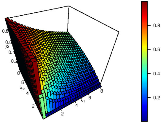
Figure 1. In this figure we graphed the $R=P(Y<X)$ with different values of parameters.

Figure 2 shows the fuzzy reliability $R_F$ as a function of the parameters ${\lambda }_1$ and ${\lambda }_2$ for different values of the fuzzy weight K. We can conclude that the fuzzy reliability $R_F$ has an upward trend with increased fuzzy weight K.

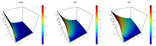
Figure 2. Fuzzy reliability of stress–strength $R_F=P(Y\prec X)$ with different values of parameters.

3. Axiomatic Classical Inference

Estimating the fuzzy reliability parameter $R_F$ is performed with the help of both the MLE and the MPS techniques presented in this section. Let $x_1,x_2,\dots ,x_n$ and $y_1,y_2,\dots ,y_m$ be two different random samples taken independently from the inverted Weibull distribution $({\lambda }_1,\beta )$ and inverted Weibull $({\lambda }_2,\beta )$, respectively.

3.1. Maximum Likelihood Estimation

The stress–strength reliability model by likelihood estimation was defined for the first time by [25]. It is possible to express the joint likelihood function of the IW distribution for the stress–strength model in the following way:

$$L({\lambda }_1,{\lambda }_2,\beta )=\prod _{i=1}^n{f}_i(x_i;{\lambda }_1,\beta )\prod _{j=1}^m{f}_j(y_j;{\lambda }_2,\beta ),$$

(6)

based on the stress–strength model, the log-likelihood ℓ function of IW is provided by

$$\begin{array}{cc}\hfill \ell (\Omega ;data)=& n\left[\log \left({\lambda }_1\right)+\log \left(\beta \right)\right]-(\beta +1)\sum _{i=1}^n{x}_i-\sum _{i=1}^n\frac{{\lambda }_1}{x_i^{\beta }}+\hfill \\ & m\left[\log \left({\lambda }_2\right)+\log \left(\beta \right)\right]-(\beta +1)\sum _{j=1}^m{y}_j-\sum _{j=1}^m\frac{{\lambda }_2}{y_j^{\beta }},\hfill \end{array}$$

(7)

where $\Omega$ is a vector of parameters $({\lambda }_1,{\lambda }_2,\beta )$. The normal equations for unknown parameters ${\lambda }_1,{\lambda }_2$, and $\beta$, and data described the sample from $x_1,\dots ,x_n$, and $y_1,\dots ,y_m$ by finding the first derivative for Equation (7) for the parameters under consideration ${\lambda }_1,{\lambda }_2$, and $\beta$, as shown in the steps below:

$$\left\{\begin{array}{c}\frac{\ell (\Omega ;data)}{\partial {\lambda }_1}=\frac{n}{{\lambda }_1}-\sum _{i=1}^n{x}_i^{-\beta }\hfill \\ \frac{\ell (\Omega ;data)}{\partial {\lambda }_2}=\frac{m}{{\lambda }_2}-\sum _{j=1}^m{y}_j^{-\beta }\hfill \\ \frac{\ell (\Omega ;data)}{\partial \beta }=\frac{n+m}{\beta }-\sum _{i=1}^n{x}_i-\sum _{j=1}^m{y}_j+\sum _{j=1}^m\frac{{\lambda }_2\log \left(y_j\right)}{y_j^{\beta }}+\sum _{i=1}^n\frac{{\lambda }_1\log \left(x_i\right)}{x_i^{\beta }}\hfill \end{array}\right.$$

(8)

Then, the estimators of ${\lambda }_1$ and ${\lambda }_2$ are given by

$${\widehat{\lambda }}_1=\frac{n}{{\sum }_{i=1}^n{x}_i^{-\beta }},\&{\widehat{\lambda }}_2=\frac{m}{{\sum }_{j=1}^m{y}_j^{-\beta }}$$

(9)

The classical reliability R and the fuzzy reliability $R_F$ of IW distribution may be produced for the stress–strength model by using the invariance property of MLE. This can be achieved by employing MLEs in the following manner:

$$\widehat{R}=\frac{{\widehat{\lambda }}_2}{{\widehat{\lambda }}_1+{\widehat{\lambda }}_2}\mathrm{and}{\widehat{R}}_F=\frac{k}{{\widehat{\lambda }}_1+k}\widehat{R}.$$

(10)

3.2. Maximum Product of Spacing Estimation

The Maximum Product of Spacing (MPS) approach was developed by Cheng and Amin [26] as a substitute for the MLE method for estimating the parameters of continuous univariate distributions. They claimed that the MPS technique possesses the majority of the maximum likelihood qualities and that the product of spacings replaces the likelihood function. The MPS technique was also independently proposed by Ranneby [9] as a way to approximate the Kullback–Leibler measure of information. The authors also noted that the MPS estimations (MPSEs) are at least as effective as the MLEs when they depart. The consistency and asymptotic features of the MPSEs are explored in [26]. The invariance property of MPSEs was studied by Coolen and Newby [27], and they claimed that it is identical to that of MLE. Additionally, the MPSEs are highly efficient, and several writers suggested using them as a good substitute for the MLE. They also discovered that in some circumstances, both in complete and censored samples, this estimating methodology can produce superior estimates than the MLE approach.

The following formula should be used to refer to the maximum product spacing for the stress–strength model.

$$\begin{array}{ccc}\hfill G(\Omega ;data)& =& {\left(\prod _{i=1}^{n+1}{D}_l(x_i,{\lambda }_1,\beta )\right)}^{\frac{1}{n+1}}{\left(\prod _{j=1}^{m+1}{D}_l(y_j,{\lambda }_2,\beta )\right)}^{\frac{1}{m+1}}.\hfill \\ \hfill \end{array}$$

(11)

The identifiable is used to describe the log-product spacing for the stress–strength model:

$$\begin{array}{ccc}\hfill G(\Omega ;data)& =& \frac{1}{n+1}\sum _{i=1}^{n+1}\log \left[e^{-\frac{{\lambda }_1}{x_i^{\beta }}}-e^{-\frac{{\lambda }_1}{x_{i-1}^{\beta }}}\right]+\frac{1}{m+1}\sum _{j=1}^{m+1}\log \left[e^{-\frac{{\lambda }_2}{y_j^{\beta }}}-e^{-\frac{{\lambda }_2}{y_{j-1}^{\beta }}}\right].\hfill \end{array}$$

(12)

To find the values of the estimates, we will use the same process as the MLEs method to obtain the normal equations. For further reading, see [27,28,29,30,31,32,33].

4. Bayesian Estimator

This section provides the Bayesian estimate of the unknown parameters ${\lambda }_1,{\lambda }_2$, and $\beta$ against the squared error and the linear, exponential loss function (LINEX); for further reading, see [34]. According to more recent papers, we assumed that the unknown parameters ${\lambda }_1,{\lambda }_2$, and $\beta$ are independent random variables with gamma prior density functions. This is done as follows:

$$\begin{array}{cc}\hfill {\pi }_1\left({\lambda }_1\right)& \propto {\lambda }_1^{a_1-1}{e}^{-b_1{\lambda }_1},{\lambda }_1>0,a_1,b_1>0,\hfill \\ \hfill {\pi }_2\left({\lambda }_2\right)& \propto {\lambda }_2^{a_2-1}{e}^{-b_2{\lambda }_2},{\lambda }_2>0,a_2,b_2>0,\hfill \\ \hfill {\pi }_3\left(\beta \right)& \propto {\beta }^{a_3-1}{e}^{-b_3\beta },\beta >0,a_3,b_3>0,\hfill \end{array}$$

where the hyperparameters $a_i,b_i,i=1,2,3$ are assigned in the simulation to constant values. To determine the proper hyperparameters for the independent joint prior, we use the estimate and variance–covariance matrix of the MLE technique. Many authors have discussed the elective hyperparameters by Dey et al. [35] and Dey et al. [36] to develop Bayesian estimation. By equating the gamma priors’ mean and variance, the estimated hyperparameters can be written as follows:

$$a_1=\frac{{\left[\frac{1}{N}{\sum }_{i=1}^N\widehat{{\lambda }_1^i}\right]}^2}{\frac{1}{N-1}{\sum }_{i=1}^N{\left[\widehat{{\lambda }_1^i}-\frac{1}{N}{\sum }_{i=1}^N\widehat{{\lambda }_1^i}\right]}^2},b_1=\frac{\frac{1}{N}{\sum }_{i=1}^N\widehat{{\lambda }_1^i}}{\frac{1}{N-1}{\sum }_{i=1}^N{\left[\widehat{{\lambda }_1^i}-\frac{1}{N}{\sum }_{i=1}^N\widehat{{\lambda }_1^i}\right]}^2},$$

$$a_2=\frac{{\left[\frac{1}{N}{\sum }_{i=1}^N\widehat{{\lambda }_2^i}\right]}^2}{\frac{1}{N-1}{\sum }_{i=1}^N{\left[\widehat{{\lambda }_2^i}-\frac{1}{N}{\sum }_{i=1}^N\widehat{{\lambda }_2^i}\right]}^2},b_2=\frac{\frac{1}{N}{\sum }_{i=1}^N\widehat{{\lambda }_2^i}}{\frac{1}{N-1}{\sum }_{i=1}^N{\left[\widehat{{\lambda }_2^i}-\frac{1}{N}{\sum }_{i=1}^N\widehat{{\lambda }_2^i}\right]}^2},$$

and

$$a_3=\frac{{\left[\frac{1}{N}{\sum }_{i=1}^N\widehat{{\beta }^i}\right]}^2}{\frac{1}{N-1}{\sum }_{i=1}^N{\left[\widehat{{\beta }^i}-\frac{1}{N}{\sum }_{i=1}^N\widehat{{\beta }^i}\right]}^2},b_3=\frac{\frac{1}{N}{\sum }_{i=1}^N\widehat{{\beta }^i}}{\frac{1}{N-1}{\sum }_{i=1}^N{\left[\widehat{{\beta }^i}-\frac{1}{N}{\sum }_{i=1}^N\widehat{{\beta }^i}\right]}^2}.$$

where N denotes the number of iterations. The posterior distribution of the parameters can be expressed as below:

$${\pi }^{*}\left({\lambda }_1,{\lambda }_2,\beta \mid data\right)=\frac{{\pi }_1\left({\lambda }_1\right){\pi }_2\left({\lambda }_2\right){\pi }_3\left(\beta \right)L({\lambda }_1,{\lambda }_2,\beta \mid x,y)}{\underset{0}{\overset{\infty }{\int }}\underset{0}{\overset{\infty }{\int }}\underset{0}{\overset{\infty }{\int }}{\pi }_1\left({\lambda }_1\right){\pi }_2\left({\lambda }_2\right){\pi }_3\left(\beta \right)L({\lambda }_1,{\lambda }_2,\beta \mid x,y)d{\lambda }_{1}d{\lambda }_{2}d\beta }.$$

(13)

where $data$ is the generated sample. It is possible to express the joint posterior to the proportionality as an equation, as shown in (13)

$$\begin{array}{cc}\hfill {\pi }^{*}\left({\lambda }_1,{\lambda }_2,\beta \mid data\right)\propto & {\beta }^{n+m+a_3-1}{e}^{-\beta \left(b_3+{\sum }_{i=1}^n\log \left(x_i\right)+{\sum }_{j=1}^m\log \left(y_j\right)\right)}{\lambda }_1^{n+a_1-1}{e}^{-{\lambda }_1\left(b_1+{\sum }_{i=1}^n{x}_i^{-\beta }\right)}\hfill \\ & \times {\lambda }_2^{m+a_2-1}{e}^{-{\lambda }_2\left(b_1+{\sum }_{j=1}^m{y}_j^{-\beta }\right)}\hfill \end{array}$$

The complete conditionals for ${\lambda }_1,{\lambda }_2$, and $\beta$ can be written, up to proportionality, as

$$\left\{\begin{array}{c}{\pi }_1^{*}\left({\lambda }_1\mid {\lambda }_2,\beta \right)\propto {\lambda }_1^{n+a_1-1}{e}^{-{\lambda }_1\left(b_1+{\sum }_{i=1}^n{x}_i^{-\beta }\right)}\hfill \\ {\pi }_2^{*}\left({\lambda }_2\mid {\lambda }_1,\beta ,data\right)\propto {\lambda }_2^{m+a_2-1}{e}^{-{\lambda }_2\left(b_2+{\sum }_{j=1}^m{y}_j^{-\beta }\right)},\hfill \\ {\pi }_3^{*}\left(\beta \mid {\lambda }_1,{\lambda }_{2}data\right)\propto {\beta }^{n+m+a_3-1}{e}^{-\beta \left(b_3+{\sum }_{i=1}^n\log \left(x_i\right)+{\sum }_{j=1}^m\log \left(y_j\right)\right)}.\hfill \end{array}\right.$$

(14)

Then,

$$\left\{\begin{array}{c}{\pi }_1^{*}\left({\lambda }_1\mid {\lambda }_2,\beta ,data\right)\propto Gamma\left(n+a_1,\left(b_1+\sum _{i=1}^n{x}_i^{-\beta }\right)\right),\hfill \\ {\pi }_2^{*}\left({\lambda }_2\mid {\lambda }_1,\beta ,data\right)\propto Gamma\left(m+a_2,\left(b_2+\sum _{j=1}^m{y}_j^{-\beta }\right)\right),\hfill \\ {\pi }_3^{*}\left(\beta \mid {\lambda }_1,{\lambda }_2,data\right)\propto Gamma\left(n+m+a_3,\left(b_3+\sum _{i=1}^n\log \left(x_i\right)+\sum _{j=1}^m\log \left(y_j\right)\right)\right).\hfill \end{array}\right.$$

(15)

The insufficiency of difference-based loss functions, such as the squared error loss, has been discussed in the recent statistical literature. Various other loss functions have been proposed. The most well-known loss function is the normalized squared loss function. The posterior mean for the $SEL$ function (symmetric) is used as the parameter estimator. As a result, when compared to the loss function, the Bayes estimates ${\lambda }_1,{\lambda }_2,\beta$, and $R_F$ are obtained based on SE and LINEX, respectively,

$$\left\{\begin{array}{c}{\tilde{\lambda }}_1=E\left({\lambda }_1\mid {\lambda }_2,\beta ,data\right),\hfill \\ {\tilde{\lambda }}_2=E\left({\lambda }_2\mid {\lambda }_1,\beta ,data\right),\hfill \\ \tilde{\beta }=E\left(\beta \mid {\lambda }_1,{\lambda }_2,data\right),\hfill \\ {\tilde{R}}_F=E\left(R_F\mid {\lambda }_1,{\lambda }_2,\beta ,data\right).\hfill \end{array}\right.$$

(16)

and

$$\left\{\begin{array}{c}{\tilde{\lambda }}_1=\frac{-1}{c}ln\left[E\left(e^{-c{\lambda }_1}\mid {\lambda }_2,\beta ,data\right)\right],\hfill \\ {\tilde{\lambda }}_2=\frac{-1}{c}ln\left[E\left(e^{-c{\lambda }_2}\mid {\lambda }_1,\beta ,data\right)\right],\hfill \\ \tilde{\beta }=\frac{-1}{c}ln\left[E\left(e^{-c\beta }\mid {\lambda }_1,{\lambda }_2,data\right)\right],\hfill \\ {\tilde{R}}_F=\frac{-1}{c}ln\left[E\left(e^{-c{R}_F}\mid {\lambda }_1,{\lambda }_2,\beta ,data\right)\right].\hfill \end{array}\right.$$

(17)

Because the above integrals are difficult to obtain, the Bayes estimate is evaluated numerically. Bayesian estimators are obtained using the Markov Chain Monte Carlo (MCMC) method. Gibbs’ sampling and more general Metropolis within Gibbs samplers are key subclasses of MCMC approaches, as discussed in [22,37]. The Metropolis–Hastings algorithm and Gibbs sampling are the two most important MCMC methods. The Metropolis–Hastings method considers that a candidate value can be generated from the IW distributions for each process iteration, similar to acceptance–rejection sampling. To produce random samples from conditional posterior densities, we make use of the Metropolis–Hastings algorithm inside the Gibbs sampling stages.

5. Generating Data for Simulations

In this part of the article, we will execute a simulation to see how well each estimate of the vector of parameters ${\lambda }_1,$${\lambda }_2$, and $\beta$ performs numerically for each approach in terms of bias, as well as the mean-squared error (MSE). The simulation algorithm may be created by the usage of the stages that are listed below.

• The values of the stress–strength of IW distribution parameters $({\lambda }_1,{\lambda }_2)$, and $\beta$ are as follows: Table 1 shows the constant ${\lambda }_1=0.5,\beta =2$, and the changes in ${\lambda }_2$ to 1.2, and 3. Table 2 shows the constant ${\lambda }_1=0.5,{\lambda }_2=0.75,\beta =2$, and ${\lambda }_1=1.5,{\lambda }_2=2,\beta =0.5$. Table 3 shows the constant ${\lambda }_1=1.5,\beta =3$, and the changes in ${\lambda }_2$ to 0.5, and 5;
  Table 1. In this table, the simulation outcomes are recorded when the initial values are ${\lambda }_1=0.5, \beta =2$.

  ${\mathit{k}}_1=0.5, {\mathit{k}}_2=3$			MLE		MPS		SE		Linex		Linex
  ${\mathbf{\lambda }}_{\mathbf{2}}$	$\mathit{n,\; m}$		Bias	MSE	Bias	MSE	Bias	MSE	Bias	MSE	Bias	MSE
  1.2	15, 10	${\lambda }_1$	0.0049	0.0277	0.0532	0.0254	0.0243	0.0287	0.0020	0.0243	0.0491	0.0355
  		${\lambda }_2$	0.1436	0.3000	0.0030	0.1417	0.1798	0.2937	0.0190	0.1463	0.3702	0.5598
  		$\beta$	0.1648	0.1558	−0.2209	0.1386	0.1514	0.1445	0.0531	0.1038	0.2583	0.2130
  		R	0.0087	0.0088	−0.0285	0.0078	0.0074	0.0083	−0.0053	0.0078	0.0205	0.0090
  		$R_{F1}$	0.0172	0.0099	−0.0210	0.0069	0.0091	0.0089	0.0096	0.0086	0.0081	0.0092
  		$R_{F2}$	0.0106	0.0103	−0.0301	0.0088	0.0059	0.0097	−0.0014	0.0092	0.0132	0.0103
  	30, 20	${\lambda }_1$	−0.0037	0.0125	0.0284	0.0121	0.0057	0.0127	−0.0020	0.0118	0.0171	0.0139
  		${\lambda }_2$	0.0731	0.1169	0.0026	0.0778	0.0969	0.1190	0.0190	0.0858	0.1873	0.1795
  		$\beta$	0.0906	0.0657	−0.1397	0.0672	0.0844	0.0639	0.0375	0.0534	0.1334	0.0800
  		R	0.0077	0.0043	−0.0160	0.0040	0.0073	0.0042	0.0005	0.0040	0.0158	0.0045
  		$R_{F1}$	0.0120	0.0046	−0.0120	0.0037	0.0086	0.0044	0.0086	0.0043	0.0081	0.0045
  		$R_{F2}$	0.0090	0.0050	−0.0169	0.0045	0.0054	0.0048	0.0013	0.0047	0.0124	0.0051
  	70, 80	${\lambda }_1$	0.0021	0.0052	0.0148	0.0052	0.0056	0.0053	0.0017	0.0051	0.0109	0.0056
  		${\lambda }_2$	0.0156	0.0199	−0.0024	0.0171	0.0214	0.0200	0.0030	0.0185	0.0406	0.0225
  		$\beta$	0.0301	0.0191	−0.0718	0.0217	0.0285	0.0188	0.0132	0.0177	0.0440	0.0205
  		R	0.0012	0.0014	−0.0074	0.0014	0.0014	0.0014	−0.0008	0.0014	0.0017	0.0014
  		$R_{F1}$	0.0028	0.0018	−0.0062	0.0016	0.0059	0.0017	0.0018	0.0017	−0.0033	0.0018
  		$R_{F2}$	0.0014	0.0018	−0.0081	0.0017	0.0011	0.0018	−0.0011	0.0018	0.0014	0.0018
  	120, 130	${\lambda }_1$	−0.0004	0.0032	0.0088	0.0032	0.0015	0.0032	−0.0011	0.0031	0.0041	0.0033
  		${\lambda }_2$	0.0099	0.0117	−0.0023	0.0106	0.0141	0.0118	0.0029	0.0112	0.0257	0.0127
  		$\beta$	0.0178	0.0110	−0.0516	0.0127	0.0177	0.0111	0.0086	0.0106	0.0268	0.0116
  		R	0.0016	0.0008	−0.0045	0.0008	0.0013	0.0008	0.0006	0.0008	0.0012	0.0008
  		$R_{F1}$	0.0027	0.0010	−0.0037	0.0010	0.0019	0.0010	0.0017	0.0010	0.0014	0.0010
  		$R_{F2}$	0.0019	0.0011	−0.0049	0.0010	0.0010	0.0011	0.0010	0.0010	0.0013	0.0011
  3	15, 10	${\lambda }_1$	0.0008	0.0297	0.0500	0.0268	0.0170	0.0295	−0.0044	0.0255	0.0404	0.0354
  		${\lambda }_2$	0.6988	3.7569	−0.2446	1.2033	0.7271	3.1044	−0.2802	0.6724	2.0324	9.9563
  		$\beta$	0.1879	0.1722	−0.2063	0.1396	0.1823	0.1634	0.0853	0.1161	0.2871	0.2371
  		R	0.0083	0.0038	−0.0359	0.0054	0.0074	0.0036	−0.0188	0.0040	0.0302	0.0040
  		$R_{F1}$	0.0200	0.0102	−0.0255	0.0079	0.0118	0.0092	0.0069	0.0089	0.0139	0.0093
  		$R_{F2}$	0.0106	0.0068	−0.0376	0.0077	0.0063	0.0064	−0.0119	0.0065	0.0208	0.0066
  	30, 20	${\lambda }_1$	−0.0006	0.0128	0.0330	0.0126	0.0087	0.0131	−0.0021	0.0122	0.0200	0.0145
  		${\lambda }_2$	0.2951	0.9614	−0.2109	0.5157	0.3682	1.0225	−0.1416	0.4119	1.0404	2.8913
  		$\beta$	0.0839	0.0686	−0.1523	0.0725	0.0842	0.0679	0.0384	0.0573	0.1321	0.0840
  		R	0.0048	0.0017	−0.0231	0.0024	0.0053	0.0017	−0.0099	0.0018	0.0207	0.0021
  		$R_{F1}$	0.0096	0.0042	−0.0191	0.0038	0.0058	0.0040	0.0026	0.0039	0.0088	0.0041
  		$R_{F2}$	0.0059	0.0030	−0.0250	0.0035	0.0043	0.0030	−0.0065	0.0030	0.0150	0.0032
  	70, 80	${\lambda }_1$	0.0018	0.0052	0.0148	0.0051	0.0058	0.0053	0.0013	0.0051	0.0103	0.0055
  		${\lambda }_2$	0.0695	0.1503	−0.1194	0.1294	0.0872	0.1569	−0.0389	0.1239	0.2277	0.2375
  		$\beta$	0.0254	0.0168	−0.0770	0.0205	0.0259	0.0169	0.0111	0.0159	0.0411	0.0183
  		R	0.0009	0.0006	−0.0101	0.0007	0.0026	0.0006	−0.0032	0.0006	0.0047	0.0006
  		$R_{F1}$	0.0026	0.0017	−0.0086	0.0016	0.0028	0.0017	0.0023	0.0017	0.0029	0.0017
  		$R_{F2}$	0.0010	0.0012	−0.0111	0.0013	−0.0021	0.0012	−0.0024	0.0012	0.0025	0.0012
  	120, 130	${\lambda }_1$	−0.0014	0.0028	0.0079	0.0027	0.0006	0.0028	−0.0012	0.0027	0.0032	0.0029
  		${\lambda }_2$	0.0643	0.0946	−0.0644	0.0817	0.0771	0.0970	−0.0010	0.0806	0.1611	0.1301
  		$\beta$	0.0217	0.0111	−0.0478	0.0122	0.0224	0.0111	0.0135	0.0106	0.0314	0.0118
  		R	0.0020	0.0003	−0.0055	0.0004	0.0020	0.0003	−0.0004	0.0003	0.0045	0.0004
  		$R_{F1}$	0.0031	0.0009	−0.0046	0.0009	0.0023	0.0009	0.0022	0.0009	0.0025	0.0009
  		$R_{F2}$	0.0023	0.0006	−0.0060	0.0007	0.0020	0.0006	0.0004	0.0006	0.0024	0.0007

  Table 2. In this table, the simulation outcomes are recorded when the initial values are.

  ${\mathit{\lambda }}_1=0.5, {\mathit{\lambda }}_2=0.75, \mathit{\beta }=2, {\mathit{k}}_1=0.5, {\mathit{k}}_2=3$
  		MLE		MPS		SE		LINEX   c = 2		LINEX   c = −2
  n, m		Bias	MSE	Bias	MSE	Bias	MSE	Bias	MSE	Bias	MSE
  15, 10	${\lambda }_1$	0.0079	0.0301	0.0553	0.0273	0.0268	0.0310	0.0044	0.0257	0.0513	0.0385
  	${\lambda }_2$	0.0661	0.1167	0.0483	0.0726	0.0970	0.1223	0.0280	0.0787	0.1771	0.1958
  	$\beta$	0.1784	0.1788	−0.2085	0.1467	0.1578	0.1609	0.0604	0.1168	0.2633	0.2333
  	R	0.0071	0.0110	−0.0158	0.0082	0.0075	0.0103	0.0015	0.0096	0.0156	0.0111
  	$R_{F1}$	0.0148	0.0091	−0.0136	0.0061	0.0087	0.0082	0.0107	0.0080	0.0064	0.0084
  	$R_{F2}$	0.0087	0.0113	−0.0185	0.0084	0.0061	0.0105	0.0027	0.0099	0.0097	0.0112
  30, 20	${\lambda }_1$	−0.0046	0.0133	0.0289	0.0130	0.0046	0.0134	−0.0060	0.0125	0.0158	0.0146
  	${\lambda }_2$	0.0155	0.0368	0.0149	0.0291	0.0339	0.0391	0.0028	0.0323	0.0683	0.0496
  	$\beta$	0.0819	0.0627	−0.1533	0.0702	0.0740	0.0608	0.0283	0.0515	0.1214	0.0750
  	R	0.0040	0.0052	−0.0110	0.0043	0.0052	0.0051	0.0011	0.0049	0.0095	0.0054
  	$R_{F1}$	0.0099	0.0042	−0.0085	0.0032	0.0076	0.0041	0.0085	0.0040	0.0062	0.0041
  	$R_{F2}$	0.0059	0.0054	−0.0120	0.0044	0.0056	0.0053	0.0024	0.0051	0.0077	0.0055
  70, 80	${\lambda }_1$	0.0017	0.0048	0.0146	0.0048	0.0046	0.0049	0.0015	0.0047	0.0105	0.0051
  	${\lambda }_2$	0.0011	0.0080	0.0070	0.0074	0.0056	0.0082	−0.0022	0.0079	0.0136	0.0087
  	$\beta$	0.0319	0.0181	−0.0703	0.0204	0.0297	0.0179	0.0148	0.0168	0.0448	0.0195
  	R	−0.0005	0.0015	−0.0047	0.0014	−0.0011	0.0015	−0.0010	0.0015	−0.0007	0.0015
  	$R_{F1}$	0.0016	0.0014	−0.0045	0.0013	0.0000	0.0014	0.0012	0.0014	−0.0011	0.0014
  	$R_{F2}$	0.0000	0.0017	−0.0056	0.0015	−0.0012	0.0017	−0.0008	0.0016	−0.0015	0.0017
  120, 130	${\lambda }_1$	0.0003	0.0029	0.0094	0.0029	0.0029	0.0030	0.0003	0.0029	0.0056	0.0030
  	${\lambda }_2$	0.0008	0.0053	0.0048	0.0050	0.0040	0.0053	−0.0007	0.0052	0.0089	0.0055
  	$\beta$	0.0182	0.0106	−0.0508	0.0122	0.0167	0.0105	0.0079	0.0101	0.0255	0.0111
  	R	0.0000	0.0010	−0.0030	0.0009	−0.0002	0.0010	−0.0005	0.0010	0.0001	0.0010
  	$R_{F1}$	0.0014	0.0009	−0.0029	0.0008	0.0005	0.0008	0.0011	0.0008	−0.0002	0.0009
  	$R_{F2}$	0.0004	0.0011	−0.0036	0.0010	−0.0002	0.0011	−0.0001	0.0011	−0.0004	0.0011
  ${\lambda }_1=1.5, {\lambda }_2=2, \beta =0.5, k_1=0.5, k_2=3$
  15, 10	${\lambda }_1$	0.1150	0.2447	−0.0592	0.1257	0.1463	0.2372	−0.0225	0.1306	0.3595	0.5044
  	${\lambda }_2$	0.2974	1.0617	−0.1307	0.4164	0.3293	0.8927	−0.1335	0.2773	0.9353	2.6420
  	$\beta$	1.6780	2.9497	1.2902	1.7569	1.5195	2.4006	1.2555	1.6072	1.6757	2.9435
  	R	0.0046	0.0115	−0.0136	0.0084	0.0051	0.0103	−0.0166	0.0079	0.0265	0.0136
  	$R_{F1}$	0.0033	0.0026	0.0077	0.0020	0.0003	0.0023	0.0046	0.0020	−0.0053	0.0025
  	$R_{F2}$	0.0016	0.0093	0.0009	0.0066	−0.0013	0.0083	−0.0038	0.0066	−0.0016	0.0101
  30, 20	${\lambda }_1$	0.0588	0.0994	−0.0374	0.0671	0.0736	0.0942	−0.0107	0.0685	0.1687	0.1445
  	${\lambda }_2$	0.1925	0.3633	−0.0542	0.2030	0.2147	0.3535	−0.0294	0.1648	0.5131	0.8275
  	$\beta$	1.5853	2.5706	1.3509	1.8712	1.4917	2.2741	1.2963	1.6999	1.5866	2.5818
  	R	0.0081	0.0055	−0.0042	0.0044	0.0087	0.0051	−0.0044	0.0041	0.0226	0.0064
  	$R_{F1}$	0.0025	0.0012	0.0053	0.0010	0.0012	0.0011	0.0034	0.0010	−0.0012	0.0012
  	$R_{F2}$	0.0041	0.0045	0.0031	0.0036	0.0029	0.0041	0.0008	0.0034	0.0047	0.0047
  70, 80	${\lambda }_1$	0.0162	0.0358	−0.0290	0.0310	0.0251	0.0345	−0.0130	0.0302	0.0656	0.0422
  	${\lambda }_2$	0.0392	0.0555	−0.0454	0.0469	0.0390	0.0527	−0.0245	0.0436	0.1027	0.0695
  	$\beta$	1.5309	2.3612	1.4287	2.0573	1.4586	2.1424	1.3164	1.7412	1.5106	2.2994
  	R	0.0019	0.0017	−0.0010	0.0016	0.0004	0.0016	−0.0010	0.0015	0.0015	0.0017
  	$R_{F1}$	0.0013	0.0005	0.0036	0.0005	0.0002	0.0005	0.0024	0.0004	−0.0023	0.0005
  	$R_{F2}$	0.0014	0.0016	0.0031	0.0015	−0.0004	0.0015	0.0017	0.0015	−0.0030	0.0016
  120, 130	${\lambda }_1$	0.0123	0.0218	−0.0172	0.0198	0.0177	0.0209	−0.0068	0.0191	0.0434	0.0240
  	${\lambda }_2$	0.0227	0.0346	−0.0347	0.0312	0.0225	0.0325	−0.0195	0.0292	0.0638	0.0388
  	$\beta$	1.5163	2.3093	1.4469	2.1030	1.4502	2.1119	1.3188	1.7448	1.4942	2.2428
  	R	0.0006	0.0010	−0.0016	0.0010	−0.0003	0.0010	−0.0014	0.0009	0.0005	0.0010
  	$R_{F1}$	0.0004	0.0003	0.0019	0.0003	−0.0002	0.0003	0.0012	0.0003	−0.0018	0.0003
  	$R_{F2}$	0.0003	0.0010	0.0012	0.0009	−0.0008	0.0009	0.0004	0.0009	−0.0024	0.0010

  Table 3. In this table, the simulation outcomes are recorded when the initial values are ${\lambda }_1=1.5, \beta =3$.

  ${\mathit{k}}_1=0.5, {\mathit{k}}_2=3$			MLE		MPS		SE		Linex		Linex
  ${\mathbf{\lambda }}_{\mathbf{2}}$	$\mathit{n,\; m}$		Bias	MSE	Bias	MSE	Bias	MSE	Bias	MSE	Bias	MSE
  0.5	15, 10	${\lambda }_1$	0.1534	0.3419	−0.0348	0.1627	0.1886	0.3457	0.0156	0.1882	0.3976	0.6597
  		${\lambda }_2$	0.0114	0.0407	0.0442	0.0331	0.0281	0.0403	−0.0007	0.0322	0.0596	0.0516
  		$\beta$	−0.7986	0.8978	−1.1912	1.5197	−0.7950	0.8877	−0.9018	0.9266	−0.6748	0.6167
  		R	−0.0069	0.0075	0.0247	0.0067	−0.0051	0.0071	0.0022	0.0065	−0.0132	0.0076
  		$R_{F1}$	0.0002	0.0010	0.0123	0.0011	−0.0006	0.0010	0.0052	0.0010	−0.0065	0.0010
  		$R_{F2}$	−0.0042	0.0047	0.0219	0.0045	−0.0044	0.0044	0.0052	0.0042	−0.0148	0.0047
  	30, 20	${\lambda }_1$	0.0488	0.0941	−0.0450	0.0658	0.0699	0.0963	−0.0073	0.0739	0.1568	0.1396
  		${\lambda }_2$	0.0078	0.0196	0.0306	0.0178	0.0197	0.0207	0.0045	0.0183	0.0360	0.0239
  		$\beta$	−0.9082	0.8847	−1.1410	1.3523	−0.6905	0.8786	−0.9564	0.9685	−0.8487	0.7836
  		R	−0.0014	0.0037	0.0183	0.0036	0.0023	0.0036	0.0037	0.0035	−0.0036	0.0037
  		$R_{F1}$	0.0007	0.0005	0.0083	0.0005	0.0004	0.0005	0.0034	0.0005	−0.0028	0.0005
  		$R_{F2}$	−0.0005	0.0022	0.0158	0.0023	−0.0028	0.0022	0.0047	0.0021	−0.0055	0.0022
  	70, 80	${\lambda }_1$	0.0203	0.0351	−0.0251	0.0300	0.0308	0.0363	−0.0024	0.0322	0.0658	0.0431
  		${\lambda }_2$	−0.0016	0.0045	0.0128	0.0045	0.0015	0.0045	−0.0025	0.0044	0.0057	0.0047
  		$\beta$	−0.7969	0.7957	−1.0717	1.1648	−0.6897	0.8495	−0.9082	0.8198	−0.6943	0.8076
  		R	−0.0019	0.0011	0.0090	0.0011	−0.0020	0.0011	0.0005	0.0011	−0.0046	0.0011
  		$R_{F1}$	−0.0001	0.0002	0.0040	0.0002	−0.0004	0.0002	0.0012	0.0002	−0.0021	0.0002
  		$R_{F2}$	−0.0012	0.0007	0.0078	0.0008	−0.0016	0.0007	0.0012	0.0007	−0.0045	0.0007
  	120, 130	${\lambda }_1$	0.0167	0.0203	−0.0131	0.0181	0.0230	0.0204	0.0034	0.0189	0.0431	0.0228
  		${\lambda }_2$	0.0023	0.0029	0.0120	0.0030	0.0014	0.0029	0.0013	0.0029	0.0056	0.0030
  		$\beta$	−0.6986	0.6983	−1.0555	1.1244	−0.5982	0.9746	−0.9929	0.9966	−0.7966	0.6945
  		R	−0.0006	0.0007	0.0067	0.0007	−0.0008	0.0007	0.0007	0.0007	−0.0022	0.0007
  		$R_{F1}$	−0.0001	0.0001	0.0027	0.0001	−0.0003	0.0001	0.0006	0.0001	−0.0013	0.0001
  		$R_{F2}$	−0.0005	0.0004	0.0055	0.0005	−0.0008	0.0004	0.0008	0.0004	−0.0025	0.0005
  5	15, 10	${\lambda }_1$	0.1411	0.2673	−0.0398	0.1298	0.1705	0.2550	0.0063	0.1426	0.3723	0.4998
  		${\lambda }_2$	0.9443	5.1602	−0.6568	4.8828	0.9240	3.2404	−1.0213	2.4227	0.8676	2.0564
  		$\beta$	−0.8350	0.8426	−1.2200	1.5916	−0.8098	0.7900	−0.9121	0.9463	−0.6930	0.6373
  		R	0.0048	0.0065	−0.0376	0.0072	0.0064	0.0059	−0.0519	0.0079	0.0491	0.0077
  		$R_{F1}$	−0.0008	0.0028	0.0018	0.0022	−0.0036	0.0026	−0.0052	0.0024	−0.0080	0.0028
  		$R_{F2}$	−0.0047	0.0077	−0.0158	0.0062	−0.0072	0.0073	−0.0295	0.0072	0.0007	0.0079
  	30, 20	${\lambda }_1$	0.0481	0.0924	−0.0456	0.0645	0.0685	0.0968	−0.0078	0.0742	0.1543	0.1392
  		${\lambda }_2$	0.7094	4.0008	−0.4500	1.9359	0.8007	3.8786	−0.6194	1.3034	0.6743	1.2747
  		$\beta$	−0.9142	0.8958	−1.1470	1.3641	−0.8971	0.8635	−0.9471	0.9512	−0.8413	0.7704
  		R	0.0073	0.0034	−0.0198	0.0035	0.0085	0.0033	−0.0281	0.0036	0.0423	0.0051
  		$R_{F1}$	0.0023	0.0014	0.0035	0.0012	0.0007	0.0014	−0.0017	0.0013	0.0016	0.0015
  		$R_{F2}$	0.0029	0.0039	−0.0054	0.0033	0.0015	0.0039	−0.0148	0.0037	0.0143	0.0043
  	70, 80	${\lambda }_1$	0.0292	0.0375	−0.0173	0.0313	0.0371	0.0375	0.0040	0.0331	0.0717	0.0447
  		${\lambda }_2$	0.1507	0.5661	−0.2917	0.4941	0.1955	0.5947	−0.2179	0.4157	0.6471	1.1386
  		$\beta$	−0.9795	0.9769	−1.0820	1.1866	−0.9698	0.9579	−0.9869	0.9912	−0.9485	0.9169
  		R	−0.0002	0.0011	−0.0106	0.0012	0.0004	0.0011	−0.0101	0.0011	0.0120	0.0013
  		$R_{F1}$	−0.0006	0.0006	0.0010	0.0005	−0.0013	0.0006	−0.0008	0.0006	−0.0015	0.0006
  		$R_{F2}$	−0.0019	0.0016	−0.0038	0.0015	−0.0025	0.0015	−0.0058	0.0015	0.0014	0.0016
  	120, 130	${\lambda }_1$	0.0148	0.0201	−0.0148	0.0180	0.0209	0.0201	0.0015	0.0187	0.0409	0.0224
  		${\lambda }_2$	0.1301	0.3287	−0.1725	0.2878	0.1566	0.3317	−0.1065	0.2470	0.4573	0.6032
  		$\beta$	−0.9798	0.9697	−1.0493	1.1101	−0.9722	0.9548	−0.9834	0.9766	−0.9571	0.9254
  		R	0.0016	0.0006	−0.0056	0.0006	0.0018	0.0006	−0.0050	0.0006	0.0092	0.0007
  		$R_{F1}$	0.0002	0.0003	0.0011	0.0003	−0.0004	0.0003	−0.0002	0.0003	−0.0004	0.0003
  		$R_{F2}$	0.0002	0.0009	−0.0013	0.0008	−0.0003	0.0008	−0.0027	0.0008	0.0023	0.0009

• The sample size of strength, n, and the sample size of stress, m are determined. The sample sizes of n = 15, 30, 70, and 120, and m = 10, 20, 80, and 130 are considered;
• The number of replications of simulation is determined, L = 10,000;
• A uniform distribution $U_1$ over the interval (0,1) is used to generate random samples of size n using the inverse of the IW distribution function in Equation (1), we transform them into samples of strength with an IW distribution with the parameters ${\lambda }_1$ and $\beta$.

  $$x_i={\left(\frac{-1}{{\lambda }_1}\log \left(u_{1i}\right)\right)}^{\frac{-1}{\beta }};i=1,\dots ,n.$$
  A uniform distribution $U_2$ with (0, 1) is used to generate random samples of size m using the inverse of the IW distribution function in Equation (1). We transform them into stress samples with an IW distribution with the parameters ${\lambda }_2$ and $\beta$.

  $$y_j={\left(\frac{-1}{{\lambda }_2}\log \left(u_{1j}\right)\right)}^{\frac{-1}{\beta }};j=1,\dots ,m.$$
• Estimate the parameters of stress–strength of IW model for each estimation method;
• Estimate traditional reliability stress–strength for each estimation method;
• Determine the parameter of membership function to give fuzzy reliability stress–strength for each estimation method as: $k_1=0.5$ is $R_{F1}$ and $k_2=3$ is $R_{F2}$;
• Calculate different measures of performance as bias and MSE for each method.

From Table 1, Table 2 and Table 3, the simulation results are concluded as follows:

• It is observed that MSE (MLE) > MSE (MPS), bias (MLE) > bias (MPS), and length of confidence interval (L.CI) of (MLE) > L.CI (MPS) in most parameters, i.e., MPS performs better than MLE in the sense of bias, MSE, and L.CI;
• It is observed that when the k value increases, the fuzzy reliability stress–strength values tend to the conventional reliability stress–strength values, which means that the uncertainty disappears;
• When the sample sizes $(n,m)$ are increased, as expected, for each parameter, the bias and MSE values decrease;
• When $k_2=3$, the fewest bias values for all calculations as well as the smallest MSE values for fuzzy and traditional reliability are found;
• It is observed that the largest MSE values for the parameters are obtained when ${\lambda }_1$ increases;
• It is observed that the smallest MSE values for the parameters are obtained when ${\lambda }_2$ increases;
• In comparison to MLE and MPS based on minimum bias and MSE, Bayesian estimators perform better;
• When ${\lambda }_1<{\lambda }_2$, reliability stress–strength value increases.

Figure 3, Figure 4 and Figure 5 present heat maps of MSE results, which conclude that the MSE decreases when the sample size increases and the Bayesian with asymmetric loss function has smallest MSE with positive weight. X-lab shows the parameters by using estimation methods. Y-lab shows the cases with different sample sizes.

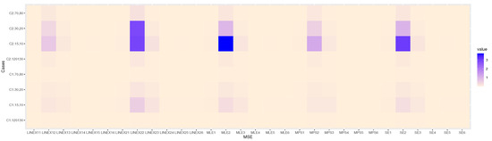
Figure 3. Heat maps of MSE results in Table 1.

Figure 4. Heat maps of MSE results in Table 2.

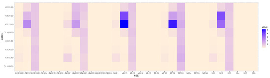
Figure 5. Heat maps of MSE results in Table 3.

6. Application of Real Data

Saraçoğlu et al. [38] and Xia et al. [39] used the following two data sets, which describe the breaking strengths of jute fiber at two different gauge lengths. The data are as follows:

Breaking strength of jute fiber of gauge length 20 mm: y = 693.73, 704.66, 323.83, 778.17, 123.06, 637.66, 383.43, 151.48, 108.94, 50.16, 671.49, 183.16, 257.44, 727.23, 291.27, 101.15, 376.42, 163.40, 141.38, 700.74, 262.90, 353.24, 422.11, 43.93, 590.48, 212.13, 303.90, 506.60, 530.55, 177.25.

Breaking strength of jute fiber of gauge length 10 mm: x = 71.46, 419.02, 284.64, 585.57, 456.60, 113.85, 187.85, 688.16, 662.66, 45.58, 578.62, 756.70, 594.29, 166.49, 99.72, 707.36, 765.14, 187.13, 145.96, 350.70, 547.44, 116.99, 375.81, 581.60, 119.86, 48.01, 200.16, 36.75, 244.53, 83.55.

Using the Kolmogrov–Smirnov (KS) test, we conclude that the IW distribution with parameter $\lambda$ = 228.7034 and $\beta$ = 1.0846 can be fitted on the strength variable, and $\lambda$ = 490.9034 and $\beta$ = 1.18304 can be fitted on the stress variable, which is shown in Table 4. Additionally, Figure 6 and Figure 7 confirmed the fitting of these data.

Table 4. MLE for each sample with the goodness of fit.

		$\mathit{\lambda }$	$\mathit{\beta }$	DKS	PKS
x	estimates	228.7034	1.084648	0.15666	0.4109
	SE	158.6319	0.146678
y	estimates	490.8034	1.183035	0.17014	0.3137
	SE	370.751	0.152611

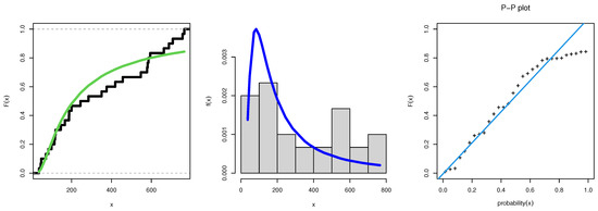
Figure 6. Estimated CDF, PDF, and p-p-plot for strength variable for the second data.

Figure 7. Estimated CDF, PDF, and pp-plot for stress variable for the second data.

Figure 6 and Figure 7 illustrate the estimated PDF and CDF of IW for stress and strength variables. It is evident from Figure 6 and Figure 7 that the IW presents a fit to the histogram of the breaking strength of the jute fiber of gauge data. The graphics in Figure 6 and Figure 7 clearly show that the closeness by P-P plot of the IW fit both stress and strength variables of breaking strength of jute fiber of gauge, emphasizing its significance in analyzing stress–strength data.

Table 5 discussed compassion of MLE, MPS, and Bayesian estimation for parameters of the IW stress–strength model with reliability goodness of fit. By standard error (SE) values, we can calculate the coefficient of variation (CV) where the CV of Bayesian estimation of parameters is the smallest value comparing CV values of MLE and MPS. Whereas, the MPS has smaller CV values than the CV values of MLE for parameters ${\lambda }_2$ and $\beta$. We know that the greatest value for the reliability of models results from the MPS method. To check the MLE values of parameters, we plotted profile likelihood to confirm these results are maximum values see Figure 8. Figure 9 shows a trace and normal curve of the posterior distribution for MCMC estimation.

Table 5. MLE, MPS, and Bayesian with reliability goodness of fit.

		${\mathit{\lambda }}_1$	${\mathit{\lambda }}_2$	$\mathit{\beta }$	R	${\mathit{R}}_{\mathit{f}1}$	${\mathit{R}}_{\mathit{f}2}$
MLE	estimates	284.8807	385.4952	1.1330	0.5750	0.2952	0.4087
	SE	146.2288	209.7269	0.1059
	CV	51.33%	54.40%	9.35%
MPS	estimates	244.1034	481.0354	1.1574	0.6634	0.3660	0.4919
	SE	130.3688	205.3030	0.1057
	CV	53.41%	42.68%	9.13%
Bayesian	estimates	331.9837	470.0805	1.1588	0.5861	0.2785	0.3975
	SE	125.8291	176.8997	0.0758
	CV	37.90%	37.63%	6.54%

Figure 8. In this figure we plotted the Profile likelihood of parameters.

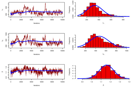
Figure 9. Iterations and Convergence of MCMC results for first data of the stress–strength model.

7. Conclusions

A novel method of calculating fuzzy stress–strength reliability $RF=P(X>Y)$ is garnering a lot of interest. This method makes the analysis more sensitive and reliable. Additionally, when the research findings are not known, the use of standard techniques may be deceptive. Therefore, it is highly vital to find new procedures that can manage such scenarios. Within the context of this study, an IW distribution was used for the stress and strength variables. It is important to keep in mind that various membership functions will, in turn, yield varying measurements. It should also be mentioned that the MPS technique outperforms the MLE and Bayesian methods in most situations.

References

- Huang, H.Z. Reliability analysis method in the presence of fuzziness attached to operating time. Microelectron. Reliab. 1995, 35, 1483–1487. [Google Scholar] [CrossRef]
- Deep, K.; Jain, M.; Salhi, S. (Eds.) Performance Prediction and Analytics of Fuzzy, Reliability and Queuing Models: Theory and Applications; Springer: Berlin/Heidelberg, Germany, 2018. [Google Scholar]
- Liu, L.; Li, X.Y.; Zhang, W.; Jiang, T.M. Fuzzy reliability prediction of rotating machinery product with accelerated testing data. J. Vibroengineering 2015, 17, 4193–4210. [Google Scholar]
- Wu, H.C. fuzzy reliability estimation using the Bayesian approach. Comput. Ind. Eng. 2004, 46, 467–493. [Google Scholar] [CrossRef]
- Wu, H.C. Fuzzy Bayesian system reliability assessment based on exponential distribution. Appl. Math. Model. 2006, 30, 509–530. [Google Scholar] [CrossRef]
- Meriem, B.; Gemeay, A.M.; Almetwally, E.M.; Halim, Z.; Alshawarbeh, E.; Abdulrahman, A.T.; El-Raouf, M.A.; Hussam, E. The power xlindley distribution: Statistical inference, fuzzy reliability, and covid-19 application. J. Functi. Sp. 2022, 2022, 9094078. [Google Scholar] [CrossRef]
- Huang, H.Z.; Zuo, M.J.; Sun, Z.Q. Bayesian reliability analysis for fuzzy lifetime data. Fuzzy Sets Syst. 2006, 157, 1674–1686. [Google Scholar] [CrossRef]
- Keller, A.Z.; Arr, K. Alternate reliability models for mechanical systems. In Proceedings of the 3rd International Conference on Reliability and Maintainability, Toulose, France, 1982. [Google Scholar]
- Keller, A.Z.; Giblin, M.T.; Farnworth, N.R. Reliability analysis of commercial vehicle engines. Reliab. Eng. 1985, 10, 15–25. [Google Scholar] [CrossRef]
- Kundu, D.; Howlader, H. Bayesian inference and prediction of the inverse Weibull distribution for Type-II censored data. Comput. Stat. Data Anal. 2010, 54, 1547–1558. [Google Scholar] [CrossRef]
- Panaitescu, E.; Popescu, P.G.; Cozma, P.; Popa, M. Bayesian and non-Bayesian estimators using record statistics of the modified-inverse Weibull distribution. Proc. Rom. Acad. Ser. A 2010, 11, 224–231. [Google Scholar]
- De Gusmao, F.R.; Ortega, E.M.; Cordeiro, G.M. The generalized inverse Weibull distribution. Stat. Pap. 2011, 52, 591–619. [Google Scholar] [CrossRef]
- Yahgmaei, F.; Babanezhad, M.; Moghadam, O.S. Bayesian estimation of the scale parameter of inverse Weibull distribution under the asymmetric loss functions. J. Probab. Stat. 2013, 2013, 890914. [Google Scholar] [CrossRef]
- Ateya, S.F. Estimation under inverse Weibull distribution based on Balakrishnan’s unified hybrid censored scheme. Commun. Stat. Simul. Comput. 2017, 46, 3645–3666. [Google Scholar] [CrossRef]
- Jana, N.; Bera, S. Interval estimation of multicomponent stress-strength reliability based on inverse Weibull distribution. Math. Comput. Simul. 2022, 191, 95–119. [Google Scholar] [CrossRef]
- Shawky, A.I.; Khan, K. Reliability Estimation in Multicomponent Stress-Strength Based on Inverse Weibull Distribution. Processes 2022, 10, 226. [Google Scholar] [CrossRef]
- Okasha, H.; Nassar, M. Product of spacing estimation of entropy for inverse Weibull distribution under progressive type-II censored data with applications. J. Taibah Univ. Sci. 2022, 16, 259–269. [Google Scholar] [CrossRef]
- Tashkandy, Y.A.; Almetwally, E.M.; Ragab, R.; Gemeay, A.M.; Abd El-Raouf, M.M.; Khosa, S.K.; Hussam, E.; Bakr, M.E. Statistical inferences for the extended inverse Weibull distribution under progressive type-II censored sample with applications. Alex. Eng. J. 2022, 65, 493–502. [Google Scholar] [CrossRef]
- Basheer, A.M.; Almetwally, E.M.; Okasha, H.M. Marshall-Olkin alpha power inverse Weibull distribution: Non-Bayesian and Bayesian estimations. J. Stat. Appl. Probab. 2021, 10, 327–345. [Google Scholar]
- Muhammed, H.Z.; Almetwally, E.M. Bayesian and non-Bayesian estimation for the bivariate inverse Weibull distribution under progressive type-II censoring. Ann. Data Sci. 2020, 10, 1–32. [Google Scholar] [CrossRef]
- El-Morshedy, M.; Eliwa, M.S.; El-Gohary, A.; Almetwally, E.M.; EL-Desokey, R. Exponentiated generalized inverse flexible Weibull distribution: Bayesian and non-Bayesian estimation under complete and type II censored samples with applications. Commun. Math. Stat. 2022, 10, 413–434. [Google Scholar] [CrossRef]
- Sabry, M.A.; Almetwally, E.M.; Alamri, O.A.; Yusuf, M.; Almongy, H.M.; Eldeeb, A.S. Inference of fuzzy reliability model for inverse Rayleigh distribution. AIMS Math. 2021, 6, 9770–9785. [Google Scholar] [CrossRef]
- Zardasht, V.; Zeephongsekul, P.; Asadi, M. On nonparametric estimation of a reliability function. Commun. Stat. Theory Methods 2012, 41, 983–999. [Google Scholar] [CrossRef]
- Neamah, M.W.; Ali, B.K. Fuzzy reliability estimation for Frechet distribution by using simulation. Period. Eng. Nat. Sci. (PEN) 2020, 8, 632–646. [Google Scholar]
- Johnson, R.A. 3 Stress-strength models for reliability. In Handbook of Statistics; Elsevier: Amsterdam, The Netherlands, 1988; Volume 7, pp. 27–54. [Google Scholar]
- Cheng, R.C.H.; Amin, N.A.K. Estimating parameters in continuous univariate distributions with a shifted origin. J. R. Stat. Soc. Ser. B (Methodol.) 1983, 45, 394–403. [Google Scholar] [CrossRef]
- Coolen, F.P.A.; Newby, M.J. A Note on the Use of the Product of Spacings in Bayesian Inference; Department of Mathematics and Computing Science, University of Technology: Eindhoven, The Netherlands, 1990; Volume 9035. [Google Scholar]
- Almongy, H.M.; Almetwally, E.M.; Alharbi, R.; Alnagar, D.; Hafez, E.H.; Mohie El-Din, M.M. The Weibull generalized exponential distribution with censored sample: Estimation and application on real data. Complexity 2021, 2021, 6653534. [Google Scholar] [CrossRef]
- Almetwally, E.M.; Jawa, T.M.; Sayed-Ahmed, N.; Park, C.; Zakarya, M.; Dey, S. Analysis of unit-Weibull based on progressive type-II censored with optimal scheme. Alex. Eng. J. 2023, 63, 321–338. [Google Scholar] [CrossRef]
- Riad, F.H.; Hussam, E.; Gemeay, A.M.; Aldallal, R.A.; Afify, A.Z. Classical and Bayesian inference of the weighted-exponential distribution with an application to insurance data. Math. Biosci. Eng. 2022, 19, 6551–6581. [Google Scholar] [CrossRef]
- Ahmad, A.; Alsadat, N.; Atchade, M.N.; ul Ain, S.Q.; Gemeay, A.M.; Meraou, M.A.; Almetwally, E.M.; Hossain, M.M.; Hussam, E. New hyperbolic sine-generator with an example of Rayleigh distribution: Simulation and data analysis in industry. Alex. Eng. J. 2023, 73, 415–426. [Google Scholar] [CrossRef]
- Beghriche, A.; Tashkandy, Y.A.; Bakr, M.E.; Halim, Z.; Gemeay, A.M.; Hossain, M.M.; Muse, A.H. The Inverse XLindley Distribution: Properties and Application. IEEE Access 2023, 11, 47272–47281. [Google Scholar] [CrossRef]
- El-Sherpieny, E.S.A.; Almetwally, E.M.; Muhammed, H.Z. Progressive Type-II hybrid censored schemes based on maximum product spacing with application to Power Lomax distribution. Phys. A Stat. Mech. Appl. 2020, 553, 124251. [Google Scholar] [CrossRef]
- Islam, A.F.M.; Roy, M.K.; Ali, M.M. A non-linear exponential (NLINEX) loss function in Bayesian analysis. J. Korean Data Inf. Sci. Soc. 2004, 15, 899–910. [Google Scholar]
- Dey, S.; Ali, S.; Park, C. Weighted exponential distribution: Properties and different methods of estimation. J. Stat. Comput. Simul. 2015, 85, 3641–3661. [Google Scholar] [CrossRef]
- Dey, S.; Singh, S.; Tripathi, Y.M.; Asgharzadeh, A. Estimation and prediction for a progressively censored generalized inverted exponential distribution. Stat. Methodol. 2016, 32, 185–202. [Google Scholar] [CrossRef]
- Salem, S.; Abo-Kasem, O.E.; Hussien, A. On Joint Type-II Generalized Progressive Hybrid Censoring Scheme. Comput. J. Math. Stat. Sci. 2023, 2, 123–158. [Google Scholar] [CrossRef]
- Saraçoğlu, B.; Kinaci, I.; Kundu, D. On estimation of R = P (Y < X) for exponential distribution under progressive type-II censoring. J. Stat. Comput. Simul. 2012, 82, 729–744. [Google Scholar]
- Xia, Z.P.; Yu, J.Y.; Cheng, L.D.; Liu, L.F.; Wang, W.M. Study on the breaking strength of jute fibres using modified Weibull distribution. Compos. Part A Appl. Sci. Manuf. 2009, 40, 54–59. [Google Scholar] [CrossRef]
Disclaimer/Publisher’s Note: The statements, opinions and data contained in all publications are solely those of the individual author(s) and contributor(s) and not of MDPI and/or the editor(s). MDPI and/or the editor(s) disclaim responsibility for any injury to people or property resulting from any ideas, methods, instructions or products referred to in the content. |
© 2023 by the authors. Licensee MDPI, Basel, Switzerland. This article is an open access article distributed under the terms and conditions of the Creative Commons Attribution (CC BY) license (https://creativecommons.org/licenses/by/4.0/).