


Solution Method for Systems of Nonlinear Fractional Differential Equations Using Third Kind Chebyshev Wavelets


Abstract
:1. Introduction
2. Operational Matrices of Fractional Integration for Third Kind Chebyshev Wavelets
2.1. Third Kind Chebyshev Wavelets
2.2. Function Approximation
2.3. Block Pulse Functions
3. Numerical Examples
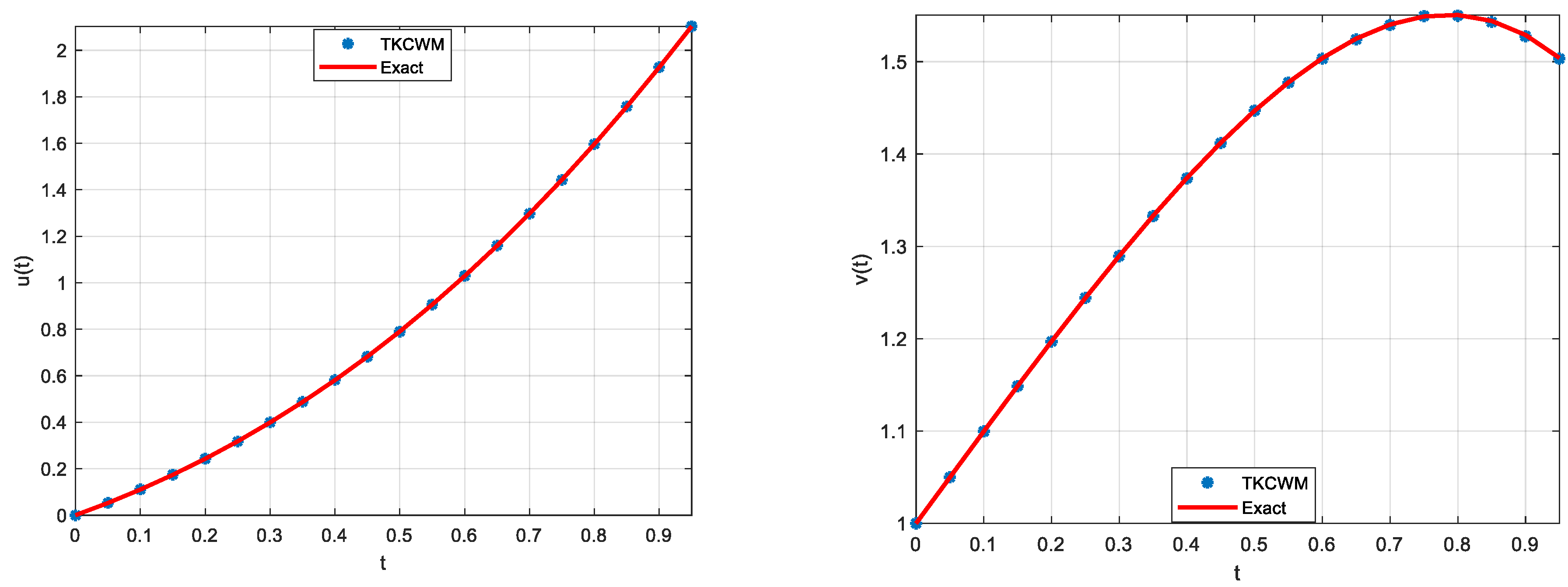
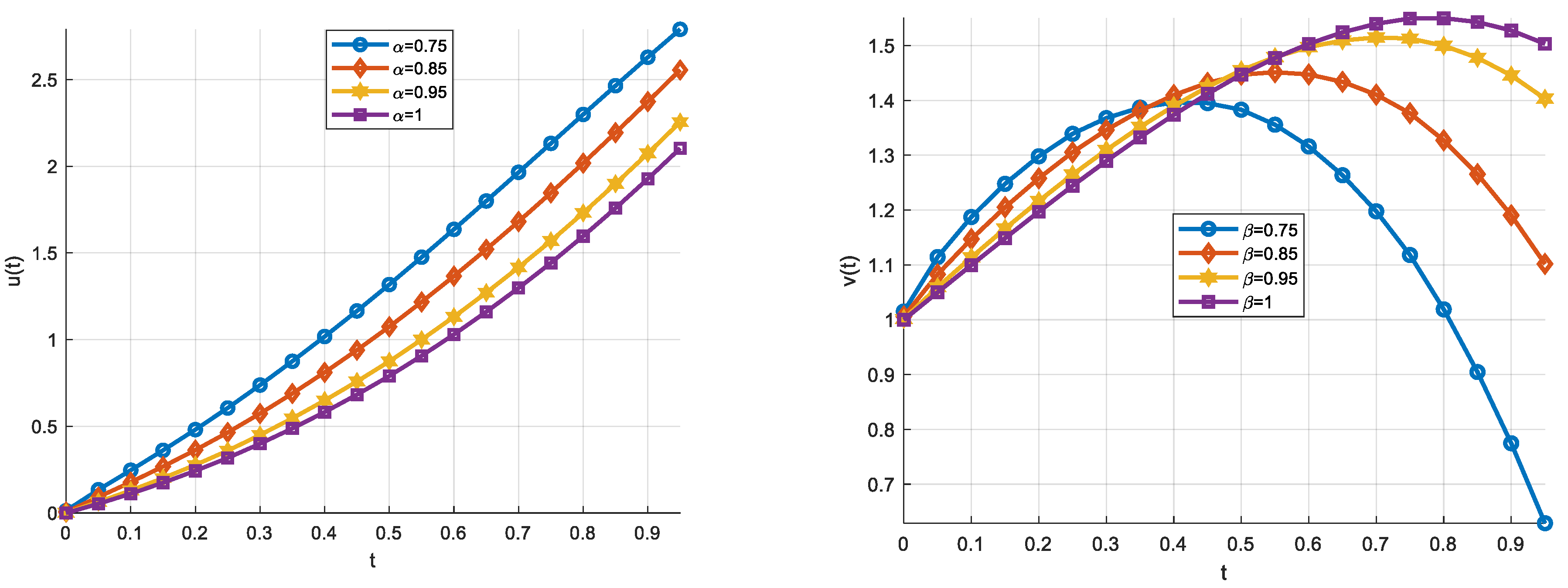
3.1. Example 1
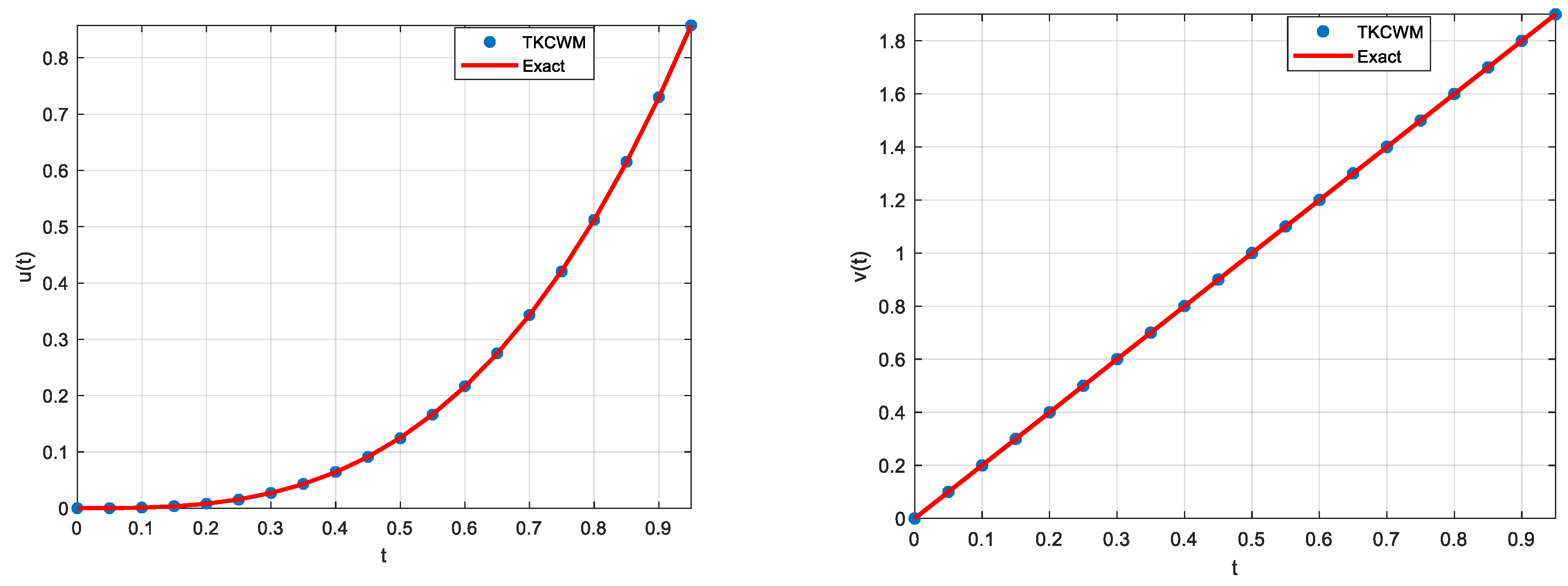
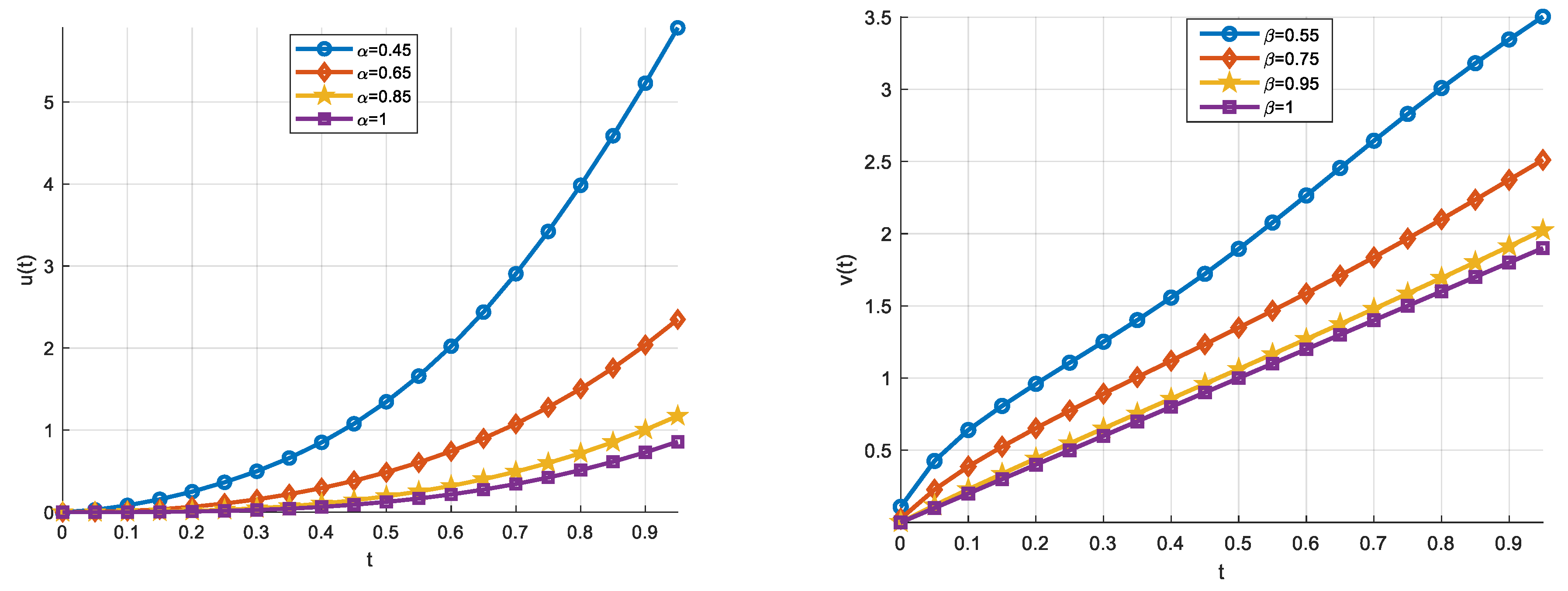
3.2. Example 2
3.3. Example 3
4. Conclusions
Author Contributions
Funding
Institutional Review Board Statement
Informed Consent Statement
Data Availability Statement
Conflicts of Interest
References
- Laoubi, M.; Odibat, Z.; Maayah, B. A Legendre-based approach of the optimized decomposition method for solving nonlinear Caputo-type fractional differential equations. Math. Methods Appl. Sci. 2022, 45, 7307–7321. [Google Scholar] [CrossRef]
- Fu, H.; Lei, T. Adomian Decomposition, Dynamic Analysis and Circuit Implementation of a 5D Fractional-Order Hyperchaotic System. Symmetry 2022, 14, 484. [Google Scholar] [CrossRef]
- Wu, G.-C.; Kong, H.; Luo, M.; Fu, H.; Huang, L.-L. Unified predictor–corrector method for fractional differential equations with general kernel functions. Fract. Calc. Appl. Anal. 2022, 25, 648–667. [Google Scholar] [CrossRef]
- Zeb, A.; Kumar, P.; Erturk, V.S.; Sitthiwirattham, T. A new study on two different vaccinated fractional-order COVID-19 models via numerical algorithms. J. King Saud Univ. Sci. 2022, 34, 101914. [Google Scholar] [CrossRef] [PubMed]
- Vargas, A.M. Finite difference method for solving fractional differential equations at irregular meshes. Math. Comput. Simul. 2021, 193, 204–216. [Google Scholar] [CrossRef]
- Kumar, S.; Kumar, R.; Agarwal, R.P.; Samet, B. A study of fractional Lotka-Volterra population model using Haar wavelet and Adams-Bashforth-Moulton methods. Math. Methods Appl. Sci. 2020, 43, 5564–5578. [Google Scholar] [CrossRef]
- Jeng, S.W.; Kilicman, A. Fractional Riccati Equation and Its Applications to Rough Heston Model Using Numerical Methods. Symmetry 2020, 12, 959. [Google Scholar] [CrossRef]
- Kaur, B.; Gupta, R.K. Dispersion analysis and improved F-expansion method for space–time fractional differential equations. Nonlinear Dyn. 2019, 96, 837–852. [Google Scholar] [CrossRef]
- Carpinteri, A.; Mainardi, F. (Eds.) Fractals and Fractional Calculus in Continuum Mechanics; Springer: Wien, NY, USA, 1997. [Google Scholar]
- Abu Arqub, O. Numerical simulation of time-fractional partial differential equations arising in fluid flows via reproducing Kernel method. Int. J. Numer. Methods Heat Fluid Flow 2019, 30, 4711–4733. [Google Scholar] [CrossRef]
- Jia, Y.-T.; Xu, M.-Q.; Lin, Y.-Z. A numerical solution for variable order fractional functional differential equation. Appl. Math. Lett. 2017, 64, 125–130. [Google Scholar] [CrossRef]
- Qin, Y.; Khan, A.; Ali, I.; Al Qurashi, M.; Khan, H.; Shah, R.; Baleanu, D. An Efficient Analytical Approach for the Solution of Certain Fractional-Order Dynamical Systems. Energies 2020, 13, 2725. [Google Scholar] [CrossRef]
- Sunthrayuth, P.; Alyousef, H.A.; El-Tantawy, S.A.; Khan, A.; Wyal, N. Solving Fractional-Order Diffusion Equations in a Plasma and Fluids via a Novel Transform. J. Funct. Spaces 2022, 2022, 1899130. [Google Scholar] [CrossRef]
- Alshorman, M.A.; Zamri, N.; Ali, M.; Albzeirat, A.K. New Implementation of Residual Power Series for Solving Fuzzy Fractional Riccati Equation. J. Model. Optim. 2018, 10, 81–87. [Google Scholar] [CrossRef]
- Bayrak, M.A.; Demir, A. A new approach for space-time fractional partial differential equations by residual power series method. Appl. Math. Comput. 2018, 336, 215–230. [Google Scholar] [CrossRef]
- Wang, Y.; Fan, Q. The second kind Chebyshev wavelet method for solving fractional differential equations. Appl. Math. Comput. 2012, 218, 8592–8601. [Google Scholar] [CrossRef]
- Yi, M.; Huang, J. Wavelet operational matrix method for solving fractional differential equations with variable coefficients. Appl. Math. Comput. 2014, 230, 383–394. [Google Scholar] [CrossRef]
- Shiralashetti, S.C.; Deshi, A.B. An efficient Haar wavelet collocation method for the numerical solution of multi-term fractional differential equations. Nonlinear Dyn. 2015, 83, 293–303. [Google Scholar] [CrossRef]
- Yuttanan, B.; Razzaghi, M. Legendre wavelets approach for numerical solutions of distributed order fractional differential equations. Appl. Math. Model. 2019, 70, 350–364. [Google Scholar] [CrossRef]
- Rahimkhani, P.; Ordokhani, Y.; Lima, P. An improved composite collocation method for distributed-order fractional differential equations based on fractional Chelyshkov wavelets. Appl. Numer. Math. 2019, 145, 1–27. [Google Scholar] [CrossRef]
- Do, Q.H.; Ngo, H.T.; Razzaghi, M. A generalized fractional-order Chebyshev wavelet method for two-dimensional distributed-order fractional differential equations. Commun. Nonlinear Sci. Numer. Simul. 2020, 95, 105597. [Google Scholar] [CrossRef]
- Usman, M.; Hamid, M.; Haq, R.U.; Wang, W. An efficient algorithm based on Gegenbauer wavelets for the solutions of variable-order fractional differential equations. Eur. Phys. J. Plus 2018, 133, 327. [Google Scholar] [CrossRef]
- Dincel, A.T.; Polat, S.N.T. Fourth kind Chebyshev Wavelet Method for the solution of multi-term variable order fractional differential equations. Eng. Comput. 2021, 39, 1274–1287. [Google Scholar] [CrossRef]
- Saeed, U.; Idrees, S.; Javid, K.; Din, Q. Krawtchouk wavelets method for solving Caputo and Caputo–Hadamard fractional differential equations. Math. Methods Appl. Sci. 2022, 45, 11331–11354. [Google Scholar] [CrossRef]
- Zhou, F.; Xu, X. The third kind Chebyshev wavelets collocation method for solving the time-fractional convection diffusion equations with variable coefficients. Appl. Math. Comput. 2016, 280, 11–29. [Google Scholar] [CrossRef]
- Boyd, J.P. Chebyshev and Fourier Spectral Methods, 2nd ed.; Courier Corporation: North Chelmsford, MA, USA, 2001. [Google Scholar]
- Kilicman, A.; Al Zhour, Z.A.A. Kronecker operational matrices for fractional calculus and some applications. Appl. Math. Comput. 2007, 187, 250–265. [Google Scholar] [CrossRef]
- Podlubny, I. Fractional Differential Equations: An Introduction to Fractional Derivatives, Fractional Differential Equations, to Methods of Their Solution and Some of Their Applications; Academic Press: New York, NY, USA, 1999. [Google Scholar]
- Ertürk, V.S.; Momani, S. Solving systems of fractional differential equations using differential transform method. J. Comput. Appl. Math. 2007, 215, 142–151. [Google Scholar] [CrossRef]
- Abdulaziz, O.; Hashim, I.; Momani, S. Solving systems of fractional differential equations by homotopy-perturbation method. Phys. Lett. A 2008, 372, 451–459. [Google Scholar] [CrossRef]


| t | ||||||||
|---|---|---|---|---|---|---|---|---|
| 0 | 2.07 × 10⁻³ | 1.34 × 10⁻⁴ | 5.04 × 10⁻⁴ | 1.60 × 10⁻⁵ | 1.24 × 10⁻⁴ | 1.95 × 10⁻⁶ | 3.08 × 10⁻⁵ | 2.41 × 10⁻⁷ |
| 0.1 | 6.76 × 10⁻⁴ | 1.52 × 10⁻⁴ | 5.09 × 10⁻⁴ | 6.85 × 10⁻⁵ | 4.14 × 10⁻⁵ | 8.49 × 10⁻⁶ | 3.19 × 10⁻⁵ | 4.35 × 10⁻⁶ |
| 0.2 | 2.27 × 10⁻³ | 6.18 × 10⁻⁴ | 1.93 × 10⁻⁴ | 7.81 × 10⁻⁵ | 1.42 × 10⁻⁴ | 3.91 × 10⁻⁵ | 1.22 × 10⁻⁵ | 5.03 × 10⁻⁶ |
| 0.3 | 2.49 × 10⁻³ | 1.06 × 10⁻³ | 2.21 × 10⁻⁴ | 1.39 × 10⁻⁴ | 1.56 × 10⁻⁴ | 6.53 × 10⁻⁵ | 1.37 × 10⁻⁵ | 8.53 × 10⁻⁶ |
| 0.4 | 9.49 × 10⁻⁴ | 8.06 × 10⁻⁴ | 6.69 × 10⁻⁴ | 3.90 × 10⁻⁴ | 6.00 × 10⁻⁵ | 5.20 × 10⁻⁵ | 4.18 × 10⁻⁵ | 2.42 × 10⁻⁵ |
| 0.5 | 2.68 × 10⁻³ | 1.11 × 10⁻³ | 6.62 × 10⁻⁴ | 2.39 × 10⁻⁴ | 1.64 × 10⁻⁴ | 5.53 × 10⁻⁵ | 4.10 × 10⁻⁵ | 1.33 × 10⁻⁵ |
| 0.6 | 1.01 × 10⁻³ | 1.58 × 10⁻³ | 7.21 × 10⁻⁴ | 7.08 × 10⁻⁴ | 6.29 × 10⁻⁵ | 9.66 × 10⁻⁵ | 4.51 × 10⁻⁵ | 4.44 × 10⁻⁵ |
| 0.7 | 2.87 × 10⁻³ | 3.61 × 10⁻³ | 2.38 × 10⁻⁴ | 4.97 × 10⁻⁴ | 1.80 × 10⁻⁴ | 2.27 × 10⁻⁴ | 1.49 × 10⁻⁵ | 3.13 × 10⁻⁵ |
| 0.8 | 2.75 × 10⁻³ | 4.53 × 10⁻³ | 2.06 × 10⁻⁴ | 6.32 × 10⁻⁴ | 1.73 × 10⁻⁴ | 2.81 × 10⁻⁴ | 1.29 × 10⁻⁵ | 3.92 × 10⁻⁵ |
| 0.9 | 6.03 × 10⁻⁴ | 3.04 × 10⁻³ | 6.27 × 10⁻⁴ | 1.37 × 10⁻³ | 3.76 × 10⁻⁵ | 1.93 × 10⁻⁴ | 3.93 × 10⁻⁵ | 8.57 × 10⁻⁵ |
| t | ||||||||
|---|---|---|---|---|---|---|---|---|
| 0 | 0.008151 | 1.008791 | 0.002943 | 1.003305 | 0.000507 | 1.00069 | −0.00012 | 1.000002 |
| 0.1 | 0.245542 | 1.188305 | 0.17689 | 1.147584 | 0.128903 | 1.113891 | 0.110374 | 1.099641 |
| 0.2 | 0.480441 | 1.298262 | 0.362622 | 1.25794 | 0.276847 | 1.216541 | 0.242798 | 1.197017 |
| 0.3 | 0.73729 | 1.367954 | 0.573061 | 1.346197 | 0.449214 | 1.309611 | 0.399066 | 1.289504 |
| 0.4 | 1.017162 | 1.397279 | 0.810237 | 1.410433 | 0.648025 | 1.390285 | 0.581004 | 1.37401 |
| 0.5 | 1.317927 | 1.38248 | 1.074454 | 1.446497 | 0.874702 | 1.454749 | 0.790275 | 1.446944 |
| 0.6 | 1.635917 | 1.317586 | 1.365448 | 1.448418 | 1.130786 | 1.497946 | 1.028909 | 1.503763 |
| 0.7 | 1.965327 | 1.198276 | 1.68092 | 1.410914 | 1.416159 | 1.515008 | 1.297475 | 1.539976 |
| 0.8 | 2.299381 | 1.019502 | 2.018072 | 1.32771 | 1.730663 | 1.500148 | 1.596678 | 1.550268 |
| 0.9 | 2.629946 | 0.77669 | 2.372987 | 1.192266 | 2.073434 | 1.447017 | 1.926711 | 1.528721 |
| t | TKCWM | DTM [29] | HPM [30] | |||
|---|---|---|---|---|---|---|
| 0 | 0.012176 | 1.00132 | 0 | 1 | 0 | 1 |
| 0.1 | 0.274122 | 1.118964 | 0.273774 | 1.11901 | 0.273774 | 1.119488 |
| 0.2 | 0.515992 | 1.203502 | 0.515442 | 1.203956 | 0.515442 | 1.207065 |
| 0.3 | 0.77603 | 1.261807 | 0.776046 | 1.265198 | 0.776046 | 1.274488 |
| 0.4 | 1.057885 | 1.291082 | 1.061045 | 1.302787 | 1.061045 | 1.322987 |
| 0.5 | 1.360936 | 1.286864 | 1.372598 | 1.315684 | 1.372598 | 1.352583 |
| 0.6 | 1.682584 | 1.244105 | 1.711912 | 1.302569 | 1.711912 | 1.362937 |
| 0.7 | 2.018624 | 1.157378 | 2.079813 | 1.262049 | 2.079813 | 1.353578 |
| 0.8 | 2.363428 | 1.021249 | 2.476944 | 1.192732 | 2.476944 | 1.323994 |
| 0.9 | 2.709949 | 0.830451 | 2.903849 | 1.093256 | 2.903849 | 1.273662 |
| t | ||||||||
|---|---|---|---|---|---|---|---|---|
| 0 | 3.66 × 10⁻⁴ | 4.77 × 10⁻⁷ | 4.58 × 10⁻⁵ | 1.49 × 10⁻⁸ | 5.72 × 10⁻⁶ | 4.66 × 10⁻¹⁰ | 7.15 × 10⁻⁷ | 1.46 × 10⁻¹¹ |
| 0.1 | 9.86 × 10⁻⁵ | 1.43 × 10⁻⁶ | 1.08 × 10⁻⁴ | 3.61 × 10⁻⁷ | 3.65 × 10⁻⁶ | 8.17 × 10⁻⁸ | 6.94 × 10⁻⁶ | 2.05 × 10⁻⁸ |
| 0.2 | 8.63 × 10⁻⁴ | 1.15 × 10⁻⁵ | 2.92 × 10⁻⁵ | 2.61 × 10⁻⁶ | 5.55 × 10⁻⁵ | 6.55 × 10⁻⁷ | 2.14 × 10⁻⁶ | 1.63 × 10⁻⁷ |
| 0.3 | 1.35 × 10⁻³ | 3.68 × 10⁻⁵ | 5.43 × 10⁻⁵ | 8.79 × 10⁻⁶ | 8.26 × 10⁻⁵ | 2.20 × 10⁻⁶ | 3.08 × 10⁻⁶ | 5.48 × 10⁻⁷ |
| 0.4 | 2.42 × 10⁻⁴ | 8.31 × 10⁻⁵ | 4.46 × 10⁻⁴ | 2.08 × 10⁻⁵ | 1.76 × 10⁻⁵ | 5.18 × 10⁻⁶ | 2.77 × 10⁻⁵ | 1.29 × 10⁻⁶ |
| 0.5 | 3.76 × 10⁻³ | 1.56 × 10⁻⁴ | 8.94 × 10⁻⁴ | 3.98 × 10⁻⁵ | 2.18 × 10⁻⁴ | 1.00 × 10⁻⁵ | 5.37 × 10⁻⁵ | 2.50 × 10⁻⁶ |
| 0.6 | 4.91 × 10⁻⁴ | 2.73 × 10⁻⁴ | 6.75 × 10⁻⁴ | 6.82 × 10⁻⁵ | 2.81 × 10⁻⁵ | 1.70 × 10⁻⁵ | 4.24 × 10⁻⁵ | 4.25 × 10⁻⁶ |
| 0.7 | 3.20 × 10⁻³ | 4.23 × 10⁻⁴ | 1.44 × 10⁻⁴ | 1.05 × 10⁻⁴ | 2.01 × 10⁻⁴ | 2.63 × 10⁻⁵ | 9.31 × 10⁻⁶ | 6.57 × 10⁻⁶ |
| 0.8 | 3.80 × 10⁻³ | 6.05 × 10⁻⁴ | 1.97 × 10⁻⁴ | 1.51 × 10⁻⁴ | 2.36 × 10⁻⁴ | 3.76 × 10⁻⁵ | 1.20 × 10⁻⁵ | 9.41 × 10⁻⁶ |
| 0.9 | 9.90 × 10⁻⁴ | 8.10 × 10⁻⁴ | 1.10 × 10⁻³ | 2.02 × 10⁻⁴ | 6.42 × 10⁻⁵ | 5.06 × 10⁻⁵ | 6.86 × 10⁻⁵ | 1.26 × 10⁻⁵ |
| t | ||||||||
|---|---|---|---|---|---|---|---|---|
| 0 | −0.00142 | 0.078944 | −0.00019 | 0.017487 | −1.7 × 10⁻⁵ | 0.001372 | −5.7 × 10⁻⁶ | −4.7 × 10⁻¹⁰ |
| 0.1 | 0.082167 | 0.63924 | 0.014506 | 0.387185 | 0.002302 | 0.229019 | 0.001004 | 0.2 |
| 0.2 | 0.249762 | 0.959284 | 0.064739 | 0.652929 | 0.015531 | 0.442512 | 0.008056 | 0.400001 |
| 0.3 | 0.497777 | 1.251181 | 0.155893 | 0.89129 | 0.047256 | 0.650949 | 0.027083 | 0.600002 |
| 0.4 | 0.84836 | 1.556029 | 0.293439 | 1.119811 | 0.104186 | 0.856963 | 0.064018 | 0.800005 |
| 0.5 | 1.338995 | 1.892988 | 0.484698 | 1.348781 | 0.192716 | 1.062435 | 0.124782 | 1.00001 |
| 0.6 | 2.015895 | 2.262136 | 0.741301 | 1.585873 | 0.320206 | 1.26917 | 0.216028 | 1.200017 |
| 0.7 | 2.898048 | 2.641492 | 1.075347 | 1.835601 | 0.492839 | 1.478814 | 0.343201 | 1.400026 |
| 0.8 | 3.974769 | 3.006082 | 1.501877 | 2.098782 | 0.71799 | 1.692719 | 0.512236 | 1.600038 |
| 0.9 | 5.21704 | 3.343328 | 2.035276 | 2.371821 | 1.00363 | 1.911611 | 0.729064 | 1.800051 |
| t | ||||||
|---|---|---|---|---|---|---|
| 0 | 6.20 × 10⁻⁵ | 2.52 × 10⁻⁴ | 5.76 × 10⁻⁴ | 1.54 × 10⁻⁵ | 6.20 × 10⁻⁵ | 1.41 × 10⁻⁴ |
| 0.1 | 2.10 × 10⁻⁵ | 8.76 × 10⁻⁵ | 2.27 × 10⁻⁴ | 1.61 × 10⁻⁵ | 6.99 × 10⁻⁵ | 1.76 × 10⁻⁴ |
| 0.2 | 7.36 × 10⁻⁵ | 3.48 × 10⁻⁴ | 9.79 × 10⁻⁴ | 6.47 × 10⁻⁶ | 2.87 × 10⁻⁵ | 8.45 × 10⁻⁵ |
| 0.3 | 8.40 × 10⁻⁵ | 4.31 × 10⁻⁴ | 1.34 × 10⁻³ | 7.81 × 10⁻⁶ | 3.65 × 10⁻⁵ | 1.20 × 10⁻⁴ |
| 0.4 | 3.78 × 10⁻⁵ | 1.90 × 10⁻⁴ | 6.94 × 10⁻⁴ | 2.40 × 10⁻⁵ | 1.34 × 10⁻⁴ | 4.63 × 10⁻⁴ |
| 0.5 | 8.54 × 10⁻⁵ | 6.30 × 10⁻⁴ | 2.30 × 10⁻³ | 2.12 × 10⁻⁵ | 1.55 × 10⁻⁴ | 5.60 × 10⁻⁴ |
| 0.6 | 5.32 × 10⁻⁵ | 3.06 × 10⁻⁴ | 1.34 × 10⁻³ | 3.12 × 10⁻⁵ | 2.07 × 10⁻⁴ | 8.72 × 10⁻⁴ |
| 0.7 | 1.42 × 10⁻⁴ | 1.03 × 10⁻³ | 4.78 × 10⁻³ | 1.58 × 10⁻⁵ | 9.85 × 10⁻⁵ | 4.76 × 10⁻⁴ |
| 0.8 | 1.61 × 10⁻⁴ | 1.27 × 10⁻³ | 6.50 × 10⁻³ | 1.85 × 10⁻⁵ | 1.25 × 10⁻⁴ | 6.57 × 10⁻⁴ |
| 0.9 | 8.73 × 10⁻⁵ | 6.39 × 10⁻⁴ | 3.70 × 10⁻³ | 4.58 × 10⁻⁵ | 3.95 × 10⁻⁴ | 2.22 × 10⁻³ |
| t | ||||||
|---|---|---|---|---|---|---|
| 0 | 1.025735 | 1.056337 | 1.113672 | 1.012877 | 1.024889 | 0.035737 |
| 0.1 | 1.495057 | 1.48695 | 2.338935 | 1.255704 | 1.597635 | 1.059627 |
| 0.2 | 1.909491 | 1.799196 | 3.573714 | 1.459601 | 2.196332 | 2.403574 |
| 0.3 | 2.370645 | 2.107951 | 5.076389 | 1.668271 | 2.919095 | 4.338173 |
| 0.4 | 2.908102 | 2.430266 | 6.94096 | 1.889877 | 3.807486 | 7.118278 |
| 0.5 | 3.546684 | 2.774319 | 9.262152 | 2.128873 | 4.904022 | 11.08098 |
| 0.6 | 4.316163 | 3.146505 | 12.16422 | 2.389192 | 6.264605 | 16.73065 |
| 0.7 | 5.245481 | 3.551287 | 15.77166 | 2.673636 | 7.945071 | 24.67848 |
| 0.8 | 6.371581 | 3.99339 | 20.24691 | 2.985366 | 10.01827 | 35.79012 |
| 0.9 | 7.73898 | 4.477634 | 25.78786 | 3.327679 | 12.57285 | 51.24301 |
Disclaimer/Publisher’s Note: The statements, opinions and data contained in all publications are solely those of the individual author(s) and contributor(s) and not of MDPI and/or the editor(s). MDPI and/or the editor(s) disclaim responsibility for any injury to people or property resulting from any ideas, methods, instructions or products referred to in the content. |
© 2023 by the authors. Licensee MDPI, Basel, Switzerland. This article is an open access article distributed under the terms and conditions of the Creative Commons Attribution (CC BY) license (https://creativecommons.org/licenses/by/4.0/).
Share and Cite
Polat, S.N.T.; Dincel, A.T. Solution Method for Systems of Nonlinear Fractional Differential Equations Using Third Kind Chebyshev Wavelets. Axioms 2023, 12, 546. https://doi.org/10.3390/axioms12060546
Polat SNT, Dincel AT. Solution Method for Systems of Nonlinear Fractional Differential Equations Using Third Kind Chebyshev Wavelets. Axioms. 2023; 12(6):546. https://doi.org/10.3390/axioms12060546
Chicago/Turabian StylePolat, Sadiye Nergis Tural, and Arzu Turan Dincel. 2023. "Solution Method for Systems of Nonlinear Fractional Differential Equations Using Third Kind Chebyshev Wavelets" Axioms 12, no. 6: 546. https://doi.org/10.3390/axioms12060546
APA StylePolat, S. N. T., & Dincel, A. T. (2023). Solution Method for Systems of Nonlinear Fractional Differential Equations Using Third Kind Chebyshev Wavelets. Axioms, 12(6), 546. https://doi.org/10.3390/axioms12060546