Article

Dynamical Analysis and Misalignment Projection Synchronization of a Novel RLCM Fractional-Order Memristor Circuit System

1
Xi’an Key Laboratory of Human-Machine Integration and Control Technology for Intelligent Rehabilitation, School of Computer Science, Xijing University, Xi’an 710123, China
2
Shaanxi International Joint Research Center for Applied Technology of Controllable Neutron Source, School of Electronic Information, Xijing University, Xi’an 710123, China
3
Frontier Institute of Science and Technology (FIST), Xi’an Jiaotong University, Xi’an 710049, China
4
Micro- and Nano-Technology Research Center, State Key Laboratory for Manufacturing Systems Engineering, Xi’an Jiaotong University, Xi’an 710049, China
*
Author to whom correspondence should be addressed.
Axioms 2023, 12(12), 1125; https://doi.org/10.3390/axioms12121125
Submission received: 23 October 2023 / Revised: 1 December 2023 / Accepted: 4 December 2023 / Published: 15 December 2023
(This article belongs to the Special Issue Advances in Theory and Applications of Chaotic and Nonlinear Dynamics)

Abstract

:
In this paper, a simple and novel fractional-order memristor circuit is established, which contains only resistance, inductance, capacitance and memristor. By using fractional calculus theory and the Adomian numerical algorithm, special bifurcations, chaotic degradation, C 0 and Spectral Entropy (SE) complexity under one-dimensional and two-dimensional parameter variations with different orders, parameters and initial memristor values of the system were studied. Meanwhile, in order to better utilize the applications of fractional-order memristor systems in communication and security, a misalignment projection synchronization scheme for fractional-order systems is proposed, which overcomes the shortcomings of constructing Lyapunov functions for fractional-order systems to prove stability and designing controllers for the Laplace transform matrix.

1. Introduction

In 1971, Leon O. Chua first proposed the existence of a fourth fundamental circuit element, in addition to the well-known capacitor, resistor and inductor. This prediction was based on his analysis of the relationship between charge and magnetic flux, following the principle that all possible variable combinations should be complete [1]. He also categorized these elements according to the properties of memristors [2]. However, the definition of implementation time is too long: it was not until 2008 that HP Labs successfully produced a nonlinear two-terminal component using nanoscale TiO 2 TiO 2 x , which confirmed the previous theoretical predictions and stimulated the research interest of domestic and foreign scholars in a memristor [3]. As a resistance with nonlinear characteristics, a memristor is a passive device. It does not only remember the amount of charge flowing through it but it also changes the resistance by controlling the current flowing through it, which is physically realizable and is considered to have the potential to subvert the traditional mode and trigger a circuit revolution. It has garnered attention in various fields including computer science [4,5], neural networks [6,7], telecommunications engineering [8,9], biological engineering [10,11] and other disciplines.
Currently, research on the preparation of memristors is a highly active area [12,13,14]. However, memristor modeling is also the key to the research, which is the basis for exploring the application of a memristor. At present, the modeling of actual memristors mostly adopts an integer-order model (only related to the information of the nearest point), that is, the equation of state of memristor internal variables adopts the form of an integer-order differential equation. In fact, if the memristor and the capacitance and inductance of dynamic circuit components adopt fractional-order models with higher degrees of freedom and better memory (information about all points in the past), they can more closely approach their actual characteristics. In 2009, Petráš et al. generalized the memristor system, memory capacitance system, and memory inductance system [15] proposed by Leon O. Chua, and obtained a fractional-order nonlinear memristor system [16]. In 2013, Fouda et al. improved the HP Ti O 2 memristor model and built a fractional memristor model, and analyzed the relationship between its memristor value and the input signal, fractional-order calculus order under different signal excitations [17,18]. In 2020, Ding et al. proposed a fractional-order memristor circuit based on the classic Chua’s circuit, analyzed its stability and dynamic characteristics and finally carried out numerical simulation, and the results were consistent with the theoretical analysis [19]. Subsequently, an increasing number of scholars focused on researching the dynamics and applications of fractional-order memristor circuit systems [20,21,22,23]. The proposal of these series of achievements not only further enriched the nonlinear circuit theory of memristors but also highlighted the complex dynamics of memristor circuits due to fractional-order sensitivity. This includes phenomena like super-multistability, coexistence/symmetry attractor, etc. Such advancements have played a crucial role in applications like image encryption, confidential communication and other engineering projects [24,25,26,27].
Chaotic synchronization belongs to a type of generalized chaos control. Chaotic synchronization theory was first developed in 1990 by Pecora and Carroll, who proposed the synchronization of chaotic circuits [28]. Chaotic synchronization can be used to achieve signal encryption at the sending end and undistorted recovery at the receiving end thanks to the sensitive initial values and noise-like properties of chaos. At present, the main methods for achieving chaos synchronization include the master-slave synchronization method [29,30], generalized synchronization method [31], the phase synchronization method [32], etc. In fact, the proportion factor between the master and slave systems determines the type of chaotic synchronization. From the perspective of secure communication, the more complex the proportion factor, the stronger the system’s anti-cracking ability. However, due to the unpredictability of its scale factors, many scholars have been conducting relevant research in recent years. Min et al. first proposed a new chaotic system synchronization method, namely, misalignment projection synchronization. Taking a new four-dimensional hyperchaotic Qi system as an example, based on Lyapunov stability theory, an effective nonlinear controller was designed to achieve the misalignment projection synchronization of two hyperchaotic Qi systems with different initial values. It has good communication and confidentiality characteristics [33]. In 2015, Sun et al. designed a feedback controller based on Lyapunov stability theory, and realized misalignment projection synchronization of a series of complex linear chaotic systems and a series of real linear chaotic systems under different initial values [34]. In 2019, Li et al. discussed mixed function projection synchronization of four-dimensional integer-order and three-dimensional integer-order chaotic systems based on Lyapunov stability theory [35]. Most of the aforementioned research focuses on misalignment projection synchronization in integer-order chaotic systems. However, given the more complex nonlinear dynamic characteristics of fractional-order memristor systems, studying their synchronization processes holds greater practical value.
In light of the above-mentioned study, this paper introduces a 3D RLCM fractional-order memristor circuit system, evolving from a basic memristor circuit [36]. This system contains just one resistor, one inductor, one capacitor and a memristor. The key advancement lies in extending the system from a limited integer-order to a fractional-order. The Adomian numerical decomposition algorithm is employed to explore the complex dynamical behaviors of the system, such as new attractors, coexisting symmetric bifurcations, Poincaré sections and Lyapunov Exponent spectra (LEs). These behaviors are analyzed under various fractional orders q, system parameters and internal memristor parameters. Secondly, the system dynamics behavior was characterized based on the C 0 algorithm and SE algorithm. Subsequently, a fractional-order misalignment projection synchronization scheme was proposed and the feasibility of the proposed scheme was verified. Finally, the paper also elaborates that the new system can be suggested for image encryption, masking and undistorted restoration due to its rich dynamics, thereby laying the foundation for further research.

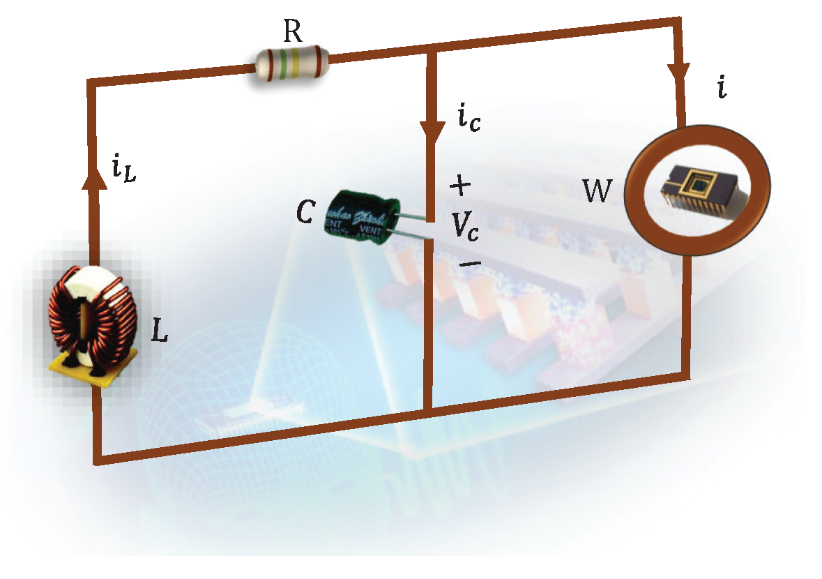
2. Fractional 3D Memristor Circuit System Model

2.1. Fractional Calculus Theory

The unified calculus includes integer-order operators and fractional-order operators, which can be represented by operator a D t 0 q , where a and t 0 are the upper and lower limits of integration, respectively, and q R is the order of the calculus operator. Calculus operators can be defined as
a D t 0 q = d q d t q , q > 0 1 , q = 0 a t d τ q , q < 0
when q > 0 , a D t 0 q represents the fractional derivative and a D t 0 q represents the fractional integral. When q = n N , then a D t 0 q is the usual integer-order derivative. In the development of fractional calculus theory, the most widely recognized definitions of fractional derivatives include the Caputo, Riemann–Liouville (RL) and Grünwald–Letnikov (GL) definitions [37,38]. Caputo defines that whether it is a fractional-order differential equation or an integer-order differential equation, its initial condition can be consistent, and it has a clear explanation of the initial condition of integer-order, and has the advantage of zero initial value when applied to constants [39]. The definition is as follows
a D t 0 q f t = 1 Γ n q a t f n τ t τ ) q n + 1 d τ
when n = q and q > 0 , according to the Caputo definition, the integral is described by the following equation.
a D t 0 q f t = 1 Γ q a t f τ t q ) 1 q d τ
and the above definition Γ is the gamma function, i.e.,
Γ z = 0 t z 1 e t d t

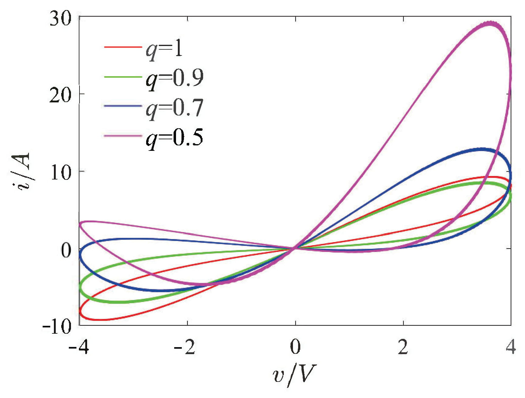
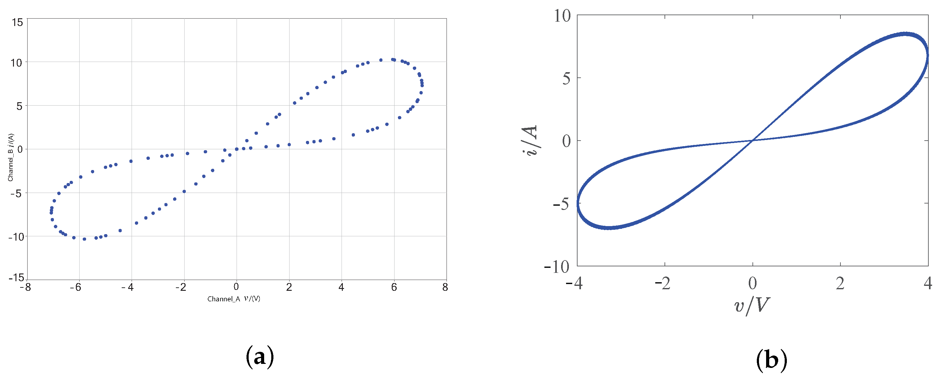
2.2. A 3D Fractional-Order Flux-Controlled Memristor

The 3D flux-controlled memristor meets the following requirements
i = d q q c φ d t = W φ v q c φ = α 3 φ 3 β 4 φ 4 φ
in which φ represents the internal state variable of memristor, q c represents charge, q represents the order, and W φ = α φ 2 β φ 3 1 represents the memristor function of the flux-controlled memristor, and v and i represent the input voltage and output current given outside the memristor, respectively. When α = 1 , β = 1 , through the numerical research on the memristor of Equation (5) above, it is found that in Figure 1, when the fractional orders are taken as q = 1 , q = 0.9 , q = 0.7 and q = 0.5 respectively, it is found that the hysteresis loop area of the memristor increases gradually in the process of the gradual reduction of the orders. Compared with integer-order, a fractional-order flux-controlled memristor has a wider range of memristor parameters, so it has the advantages of easy integration and low power consumption.
Further, according to Kirchhoff’s voltage law, we set the circuit parameters of memristor as shown in Table 1.
Based on Equation (5), the circuit schematic for the 3D fractional-order flux-controlled memristor can be designed, as shown in Figure 2.
Here, the terms A i ( i = 1 , 2 , 3 , 4 , 5 ) represent multipliers and U i ( i = 1 , 2 , 3 , 4 ) denote amplifiers. From the circuit schematic of the 3D fractional-order flux-controlled memristor, the following input–output circuit equation of the memristor can be derived. The numerical simulation and circuit simulation v ( t ) - i ( t ) curves are shown in Figure 3, further verifying the correctness of the 3D flux-controlled memristor model proposed in this paper.
i t = R 6 R 5 R 2 R 7 φ 2 v t R 4 R 3 R 2 R 8 φ 3 v t R 2 R 1 v t

2.3. Fractional-Order System Description and Chaotic Description

Based on the 3D fractional-order flux-controlled memristor circuit system [36], a simple and novel fractional-order memristor chaotic circuit system that only includes resistance, inductance, capacitance and a memristor is established. Its circuit principle is shown in Figure 4.
In the above circuit schematic diagram, the symbols R, L and C represent the resistance, inductance and capacitance of the system, respectively. It can be seen from the above that the system is shown in Equation (5), and d φ d t = v c ι φ + κ v c φ . According to Kirchhoff’s voltage law in Figure 4, the following fractional-order memristor circuit system can be obtained.
d q v c d t = 1 C i L W φ v c d q i L d t = 1 L v c R i L d q φ d t = v c ζ φ + ξ v C φ
We introduce four state variables into the circuit equation for dimensionless processing, so that x 1 = v c , x 2 = i L , x 3 = φ . And the 3D flux-controlled fractional memristor is W φ = α φ 2 β φ 3 1 and capacitance C = 1 , inductance L = 1 , R = 0.4 , ζ = a = 1 , ξ = b = 4 , and the internal parameters of the memristor are α = 1 and β = 1 . Thus, Equation (7) can be written as a dimensionless equation.
D t 0 q x 1 = x 2 α x 3 2 β x 3 3 1 x 1 D t 0 q x 2 = x 1 0.4 x 2 D t 0 q x 3 = x 1 a x 3 + b x 1 x 3
According to the Caputo fractional-order differential definition in Equation (2), when t t 0 , t 1 , k 1 < q < k k N , the two basic properties of the Caputo operator are as follows
D t 0 q J t 0 q x t = x t
and
J t 0 q D t 0 q x t = x t κ 1 k = 0 x κ t 0 +
where the k = 0 κ 1 x k t 0 + denotes a summation, representing the total of all terms from k down to 0. This notation is mathematically accurate and signifies the sum of the first k derivatives of the function x t evaluated at t 0 + , which is a moment shortly after t 0 . The Adomian decomposition algorithm is applied to analyze the system as described in system (8). By assuming a decomposition into three terms, we derive the following initial value problem.
D t 0 q x t + L x t + N x t = Λ t x k t 0 + = b k , k = 0 , 1 , , m 1 m N , m 1 < q m
In this, D t 0 q represents the q order Caputo derivative, while L and N represent the linear and nonlinear terms of system (8), respectively.
L x 1 L x 2 L x 3 = x 2 + x 1 x 1 0.4 x 2 x 1 a x 3 , N x 1 N x 2 N x 3 = α x 1 x 3 2 β x 1 x 3 3 0 b x 1 x 3 , Λ 1 Λ 1 Λ 1 = 0 0 0
And the initial value vector of system (8) is Λ x 1 Λ x 2 Λ x 3 T = 0 0 0 T , so it can be inferred from Equation (12) that Equation (13) holds as follows
D t 0 q x t = Λ t L x t N x t
By combining Equations (10) and (13), the following Equation (14) can be obtained.
x t = k = 0 m 1 b k t t 0 k k ! + J t 0 q Λ t J t 0 q L x t J t 0 q N x t
According to Equation (12), system (8) can be rewritten as
x 1 t x 2 t x 3 t = x 1 t 0 x 2 t 0 x 3 t 0 + J t 0 q x 2 + x 1 x 1 0.4 x 2 x 1 a x 3 + J t 0 q α x 1 x 3 2 β x 1 x 3 3 0 b x 1 x 3
For the linear term L x ( t ) and nonlinear term N x ( t ) of system (8), they can be expressed as
x = i = 0 x i = i = 0 x 1 i , x 2 i , x n i T
N x = i = 0 A i = i = 0 A 1 i , A 2 i , A n i T
Combined with the rate of convergence of the Adomian algorithm for a fractional-order system, the first five items of system (8) are selected under the condition of ensuring accuracy, and among them are the nonlinear terms x 1 x 3 2 , x 1 x 3 3 and x 1 x 3 . Following the principle of nonlinear term decomposition [40,41], the decomposition process is detailed in Appendix A. Substituting Equations (16) and (17) into Equation (14), the infinite series solution of system (8) is as follows
x = i = 0 x i = k = 0 m 1 b k t t 0 k k ! + J t 0 q Λ t J t 0 q L i = 0 x i J t 0 q L i = 0 A i
According to Equation (18), the recursive form of x ( t ) is as follows
x 0 = k = 0 m 1 b k t t 0 k k ! + J t 0 q Λ t x 1 = J t 0 q L x 0 J t 0 q A 0 x 2 = J t 0 q L x 1 J t 0 q A 1 x i = J t 0 q L x i J t 0 q A i
Therefore, Equation (19) provides an infinite series solution to Equation (16). Thus, in the interval t t 0 , t 1 , the infinite series solution of Equation (16) can be rewritten as
x j t = i x j i = x j 0 + x j 1 + x j 2 + x j 3 + + x j i + , j = 1 , , n
According to the initial condition, x 0 is equivalent to x 0 = x 1 t 0 , x 2 t 0 , x 3 t 0 , and the decomposition coefficient of the system (8) is shown in Appendix B. Then, by selecting the first five terms in the series Equation (20), the approximate solution of system (8) in the interval t 0 , t 1 is
x ˜ 1 t = x 1 0 + x 1 1 + x 1 2 + x 1 3 + x 1 4 + x 1 5 x ˜ 2 t = x 2 0 + x 2 1 + x 2 2 + x 2 3 + x 2 4 + x 2 5 x ˜ 3 t = x 3 0 + x 3 1 + x 3 2 + x 3 3 + x 3 4 + x 3 5
Using the Adomian decomposition algorithm and considering system (8) with parameters set to a = 1 , b = 4 , and fractional order q = 0.55 , the internal parameters of the memristor are set to α = 1 , β = 1 . Setting the initial values of the system to x 0 = ( 0.01 , 0.1 , 0 ) , the phase diagram of the system, as shown in Figure 5, can be obtained, where system (8) is chaotic.
Figure 6a,b show the results of Poincaré section with x 2 = 0 and x 3 = 0 , respectively, when the fractional orders are q = 0.3 and q = 0.9 , and the remaining parameters of the system remain consistent with the above. There are some irregular point distributions in the Poincaré section of the system, both at the three-dimensional interface and on the plane, further explaining the complex dynamic behavior of the system caused by fractional order q.

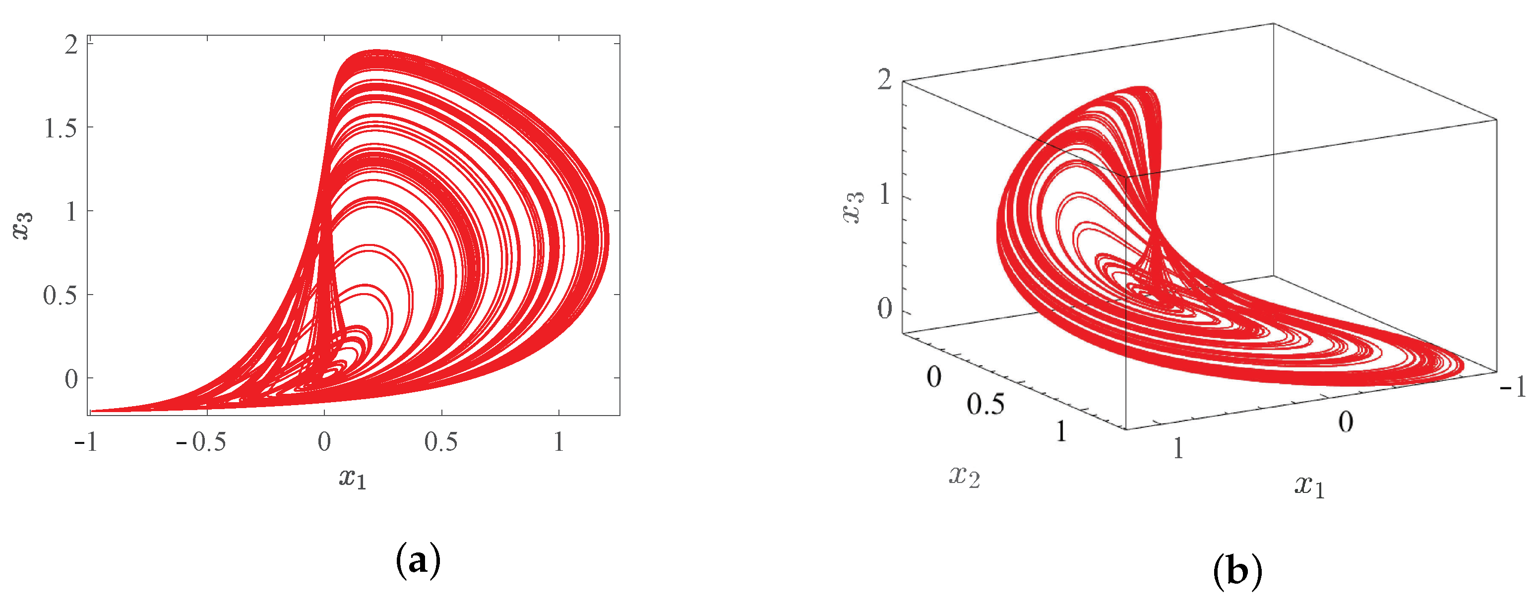
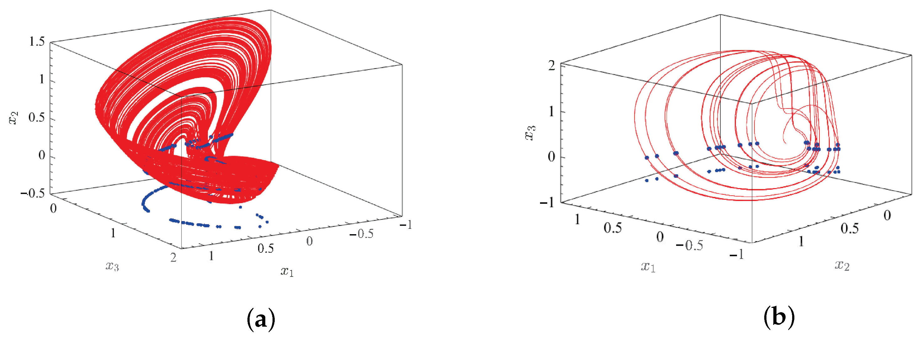
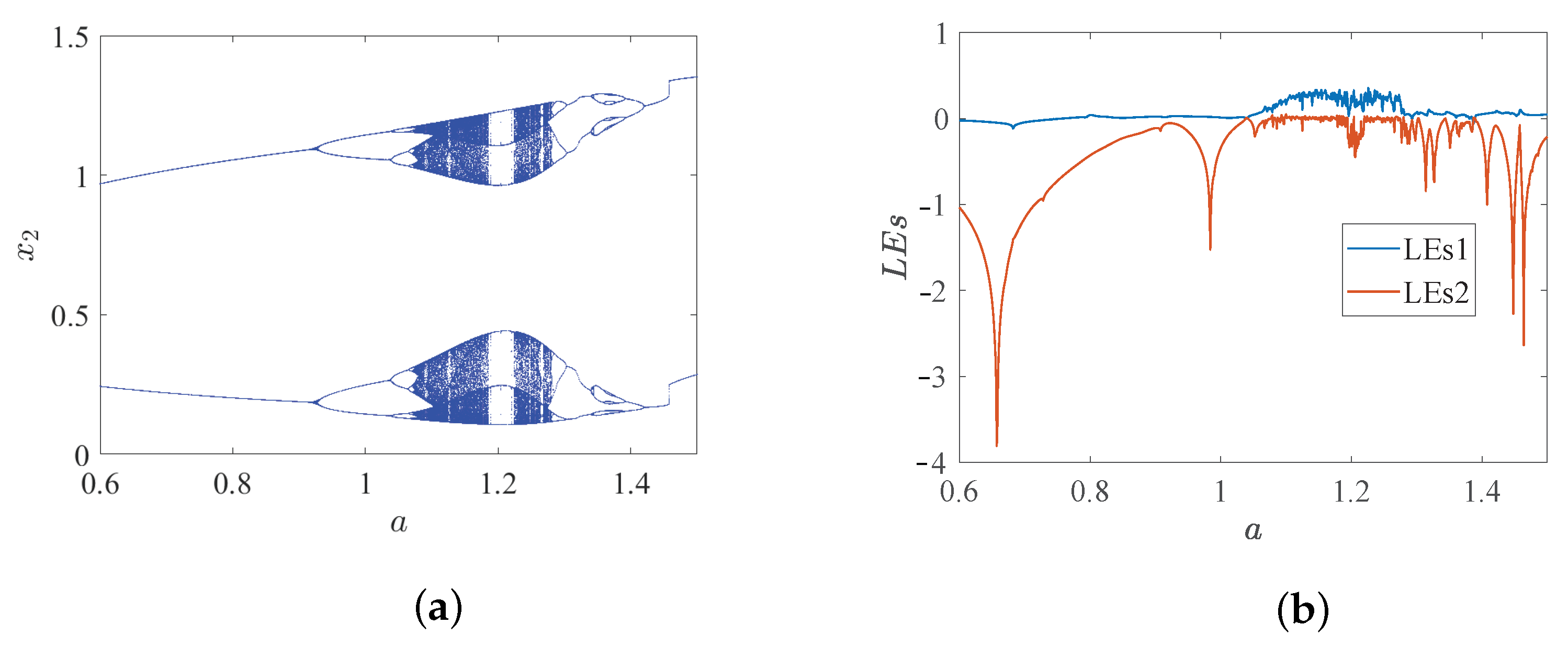
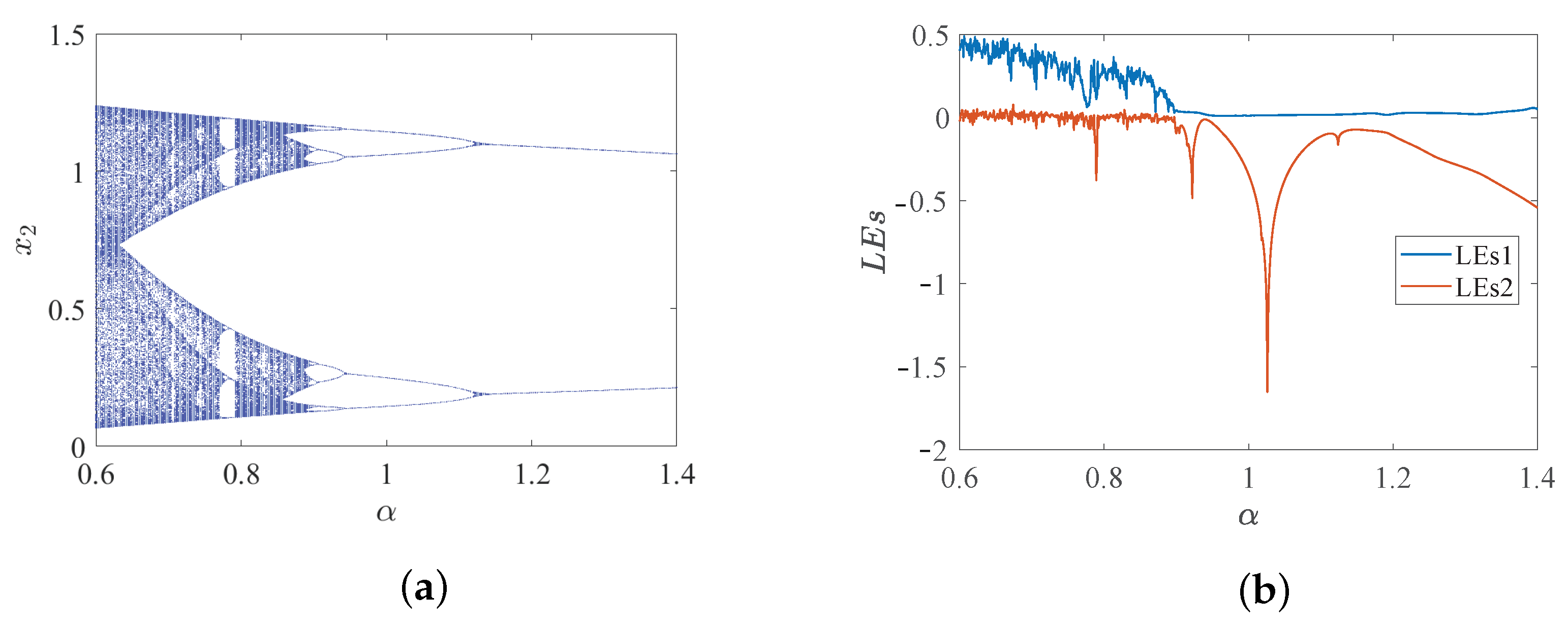
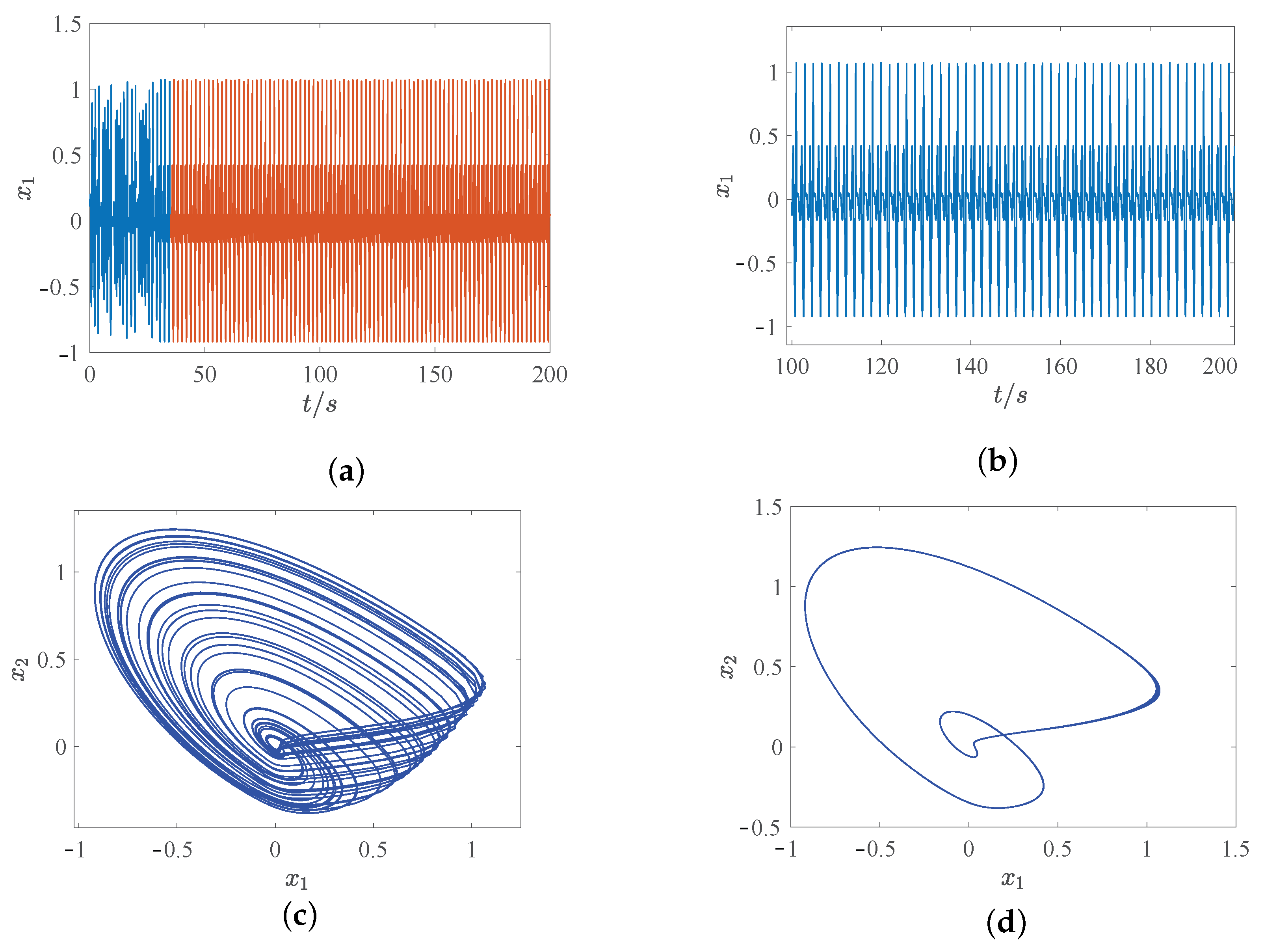
3. System Dynamics Behavior

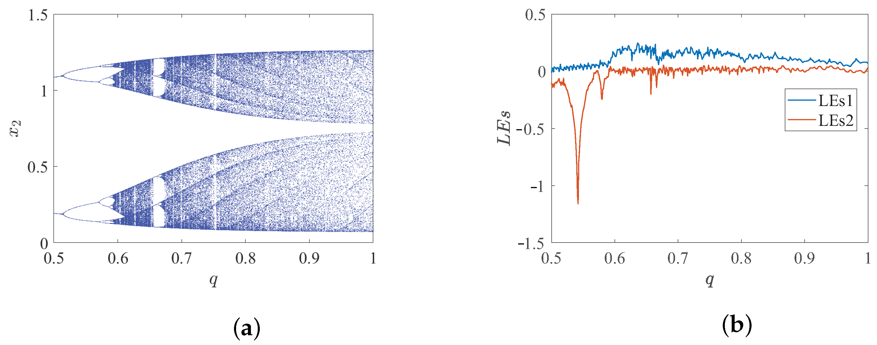
3.1. Special Bifurcation Phenomenon of the System

To analyze the dynamic phenomenon of order q changes in fractional-order memristor system, when the range of order change q ( 0.5 , 1 ) , a = 1 , b = 4 , α = 1 and β = 1 , we set the initial value of the system to x 0 = ( 0.01 , 0.1 , 0 ) . Figure 7 shows the bifurcation and LEs as the fractional order q changes: Figure 7a shows two period-doubling bifurcation paths with upper and lower symmetric synchronization paths, and a brief period window appears on their paths, ultimately ending in a chaotic state; the results in Figure 7b and the bifurcation diagram reflect consistent dynamic results.
Utilizing the 0-1 testing method, this method is mainly a quantitative analysis method to determine whether the system has chaotic or periodic motion states. As shown in Figure 8, the parameter values and initial values of the system remain consistent with the aforementioned. When the order q = 0.55 is selected on the bifurcation path of the fractional-order memristor system, the trajectory in the p-s plane is ordered. When the order q = 0.62 , the trajectory of the system in the p-s plane is chaotic and disorderly. It separately explains why the two motion states of system (8) exhibit periodic and chaotic phenomena under two sets of the order q values.
When parameter q = 0.55 , b = 4 , and the internal parameter of memristor α = 1 , β = 1 , we set the initial value of the system to x 0 = ( 0.01 , 0.1 , 0 ) . When the system parameter a is a variable, Figure 9a shows a bifurcation diagram of the variation of parameter a, describing the system changing within the range of parameter a ( 0.6 , 1.5 ) ,; it indicates a novel bifurcation phenomenon where the bifurcation path of the system with parameter a exhibits a symmetric period doubling bifurcation and ends with a reverse period doubling bifurcation. Furthermore, in conjunction with the spectral lines of the first two Lyapunov Exponents (LEs) shown in Figure 9b, it is observed that the bifurcation diagram exhibits consistent dynamic behavior.
Similarly, the internal parameter α of memristor W φ = α φ 2 β φ 3 1 is selected as a variable to research the dynamic behavior of the system. When selecting α ( 0.6 , 1.4 ) , Figure 10 shows the internal parameter α of the memristor, respectively. The bifurcation diagram is a variable and so are the first two largest spectrum lines of LEs. It can be observed that the overall dynamic behavior of the system exhibits a process of reverse period doubling bifurcation, which shows that the internal parameters of the memristor in this system have a great impact on the dynamic phenomenon of the system.

3.2. Chaotic Degradation Phenomenon of the System

The nonlinear memristor chaotic system is in a chaotic state within a finite time range, and after a period of time, it sinks into a periodic state (chaotic degradation). To illustrate the chaotic degenerate dynamic behavior of the system (8), we set the parameters of the system as a = 1 , b = 4 , fractional order q = 0.545 and α = 1 , β = 1 , respectively. The initial value of the system is set to x 0 = ( 0.1 , 0 , 0 ) . Therefore, the time-domain waveform of the system state variable x 1 is shown in Figure 11, while selecting the phase diagram of the system on the x 1 - x 2 plane at the same time. In order to verify the chaotic degradation dynamic behavior, the LEs time-domain waveform of system (8) was further obtained. In Figure 11a, it is found that the chaotic phenomenon appears before t < 35   s , and it degenerates to a periodic state after t > 35   s .
Meanwhile, the time domain waveform of time t ( 100   s 200   s ) is obtained as shown in Figure 11b. The time domain waveform changes regularly, indicating a stable periodic state. Additionally, the interval phase diagrams in Figure 11c,d reveal that the results align with the time-domain waveforms. It is further observed that the chaotic attractor emerges before t < 35   s , while a stable periodic limit cycle state manifests after t > 35   s .

4. System Complexity Analysis

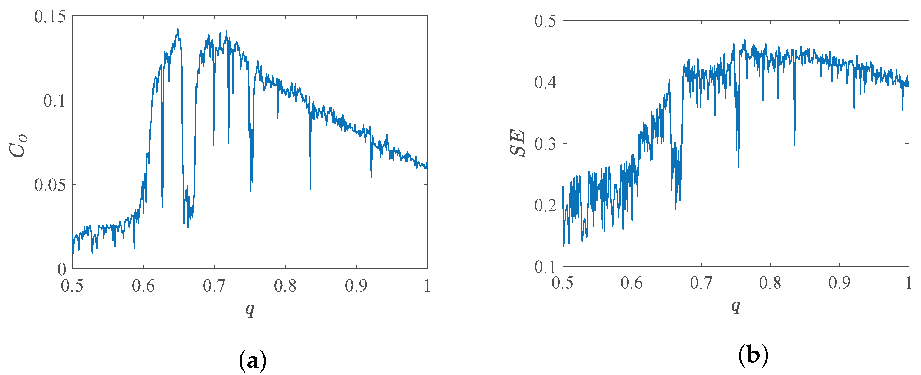
4.1. Characteristics of Complexity Variation with Order q

Any description of the nonlinear dynamic behavior of a system can be considered research into the complexity of the system. Complexity actually involves exploring whether a chaotic sequence is close to a random sequence. If it is closer to a random sequence, it indicates that the complexity of the system is relatively high. When the parameters of system (8) are consistent with the parameters researched in Figure 7, the C 0 complexity and SE complexity of the system with respect to fractional order q are shown in Figure 12. The smaller the order, the smaller the system complexity, and vice versa, which is consistent with the dynamic characteristics described by the Largest Lyapunov exponent (LLE) of fractional order q as a variable in Figure 7.
Then, we found that Figure 12 was researched using the C 0 complexity algorithm and the SE complexity algorithm. Through comparative research between the two algorithms, it was found that they can reflect the same dynamic behavior, but what can be found is that the C 0 complexity characterizes the dynamic phenomenon more effectively.

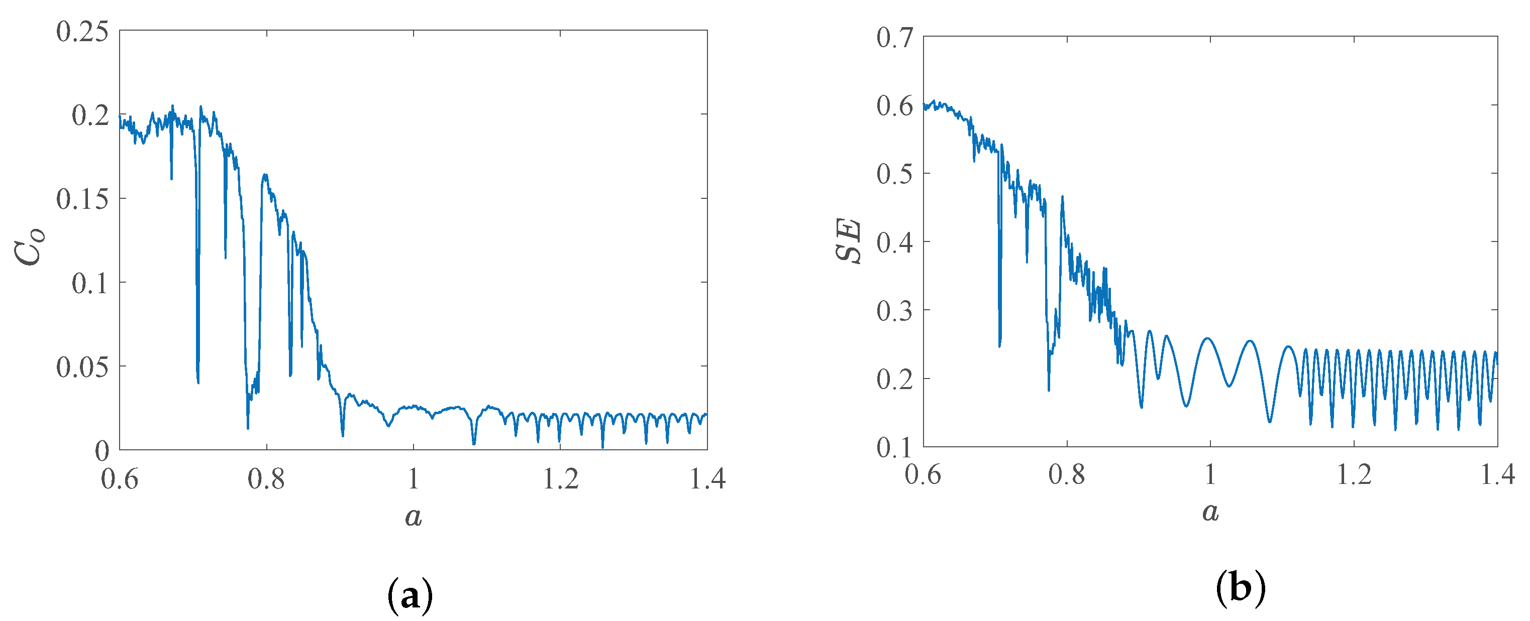
4.2. Characteristics of Complexity Variation with Internal Parameter α of Memristor

Similarly, when the system parameters are consistent with the above, according to the internal parameters of the system memristor α , the C 0 complexity and SE complexity can be determined and they are shown in Figure 13. Furthermore, we can find the internal parameters of the system memristor α the LLE under changes, as shown in Figure 10, showing good consistency between the structural complexity and the dynamic characteristics described by the LLE.

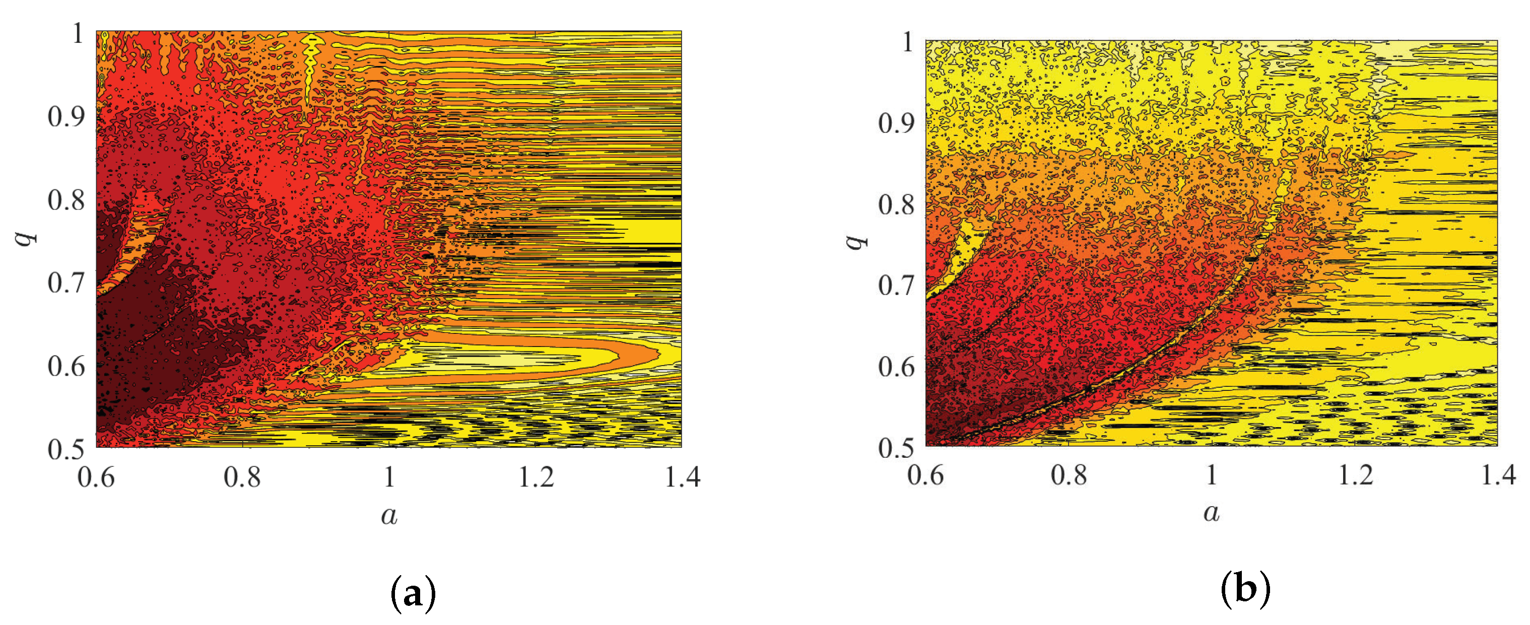
4.3. Chaotic Map of System Complexity

Based on the C 0 algorithm and SE algorithm, the complexity chaos diagram of the system can be determined, as shown in Figure 14, and the system parameter settings are consistent with the dynamic phenomena researched above. It can be seen from Figure 14 that the chaotic region of the system is basically concentrated in the fractional order q ( 0.55 , 0.8 ) and the internal parameters of the system memristor α ( 0.6 , 0.8 ) . In this region, the system exhibits a small dark-red area that exhibits complex chaotic behavior, and the boundary between the high complexity and low complexity regions of the system can be clearly determined through the complexity chaotic map.

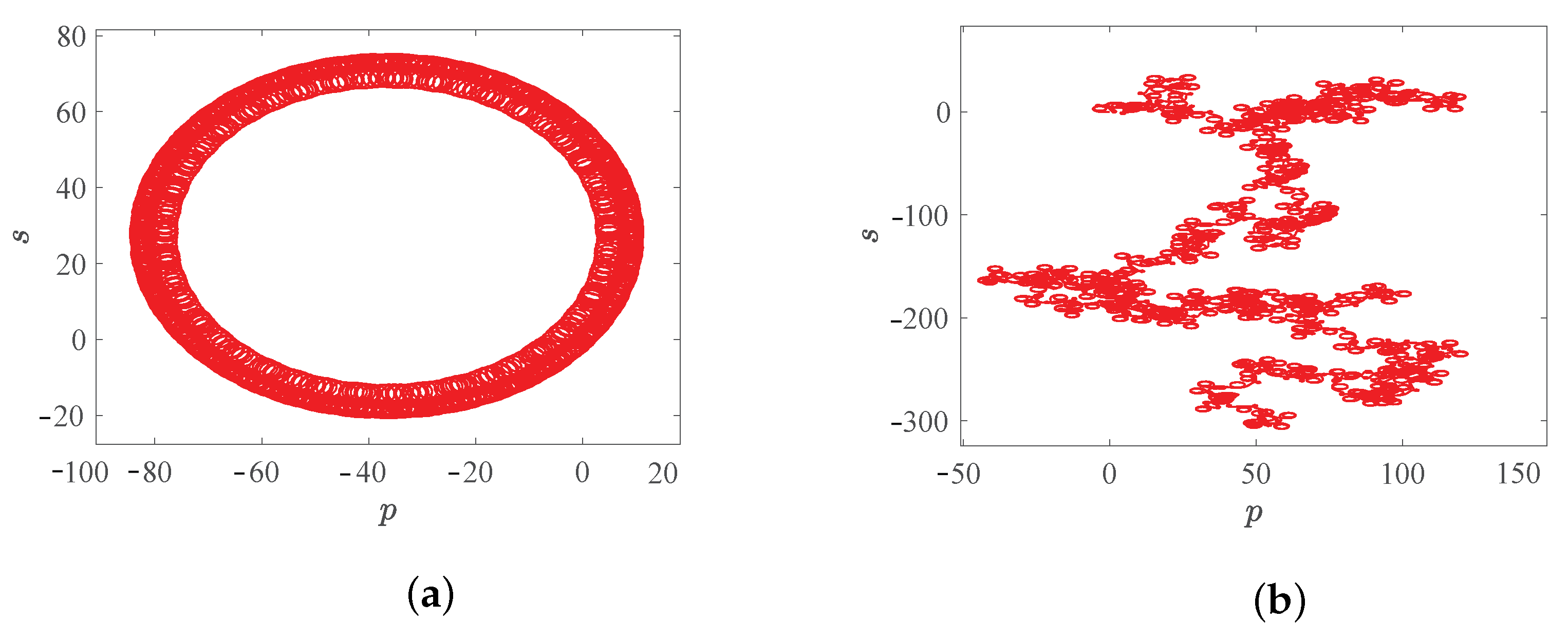
5. Misalignment Projection Synchronization of the System

5.1. Theoretical Analysis of Misalignment Projection Synchronization

Definition 1. 
If there is a fractional-order chaotic system D t 0 q x = f x , x R n is a fractional-order system variable. If the nonlinear function is selected as f : R n R n , the slave system of the fractional-order system can be defined as D t 0 q y = f y + U , and U is the controller. Therefore, the fractional-order error system is defined as follows
e t = y Φ x
In which, Φ for n × n constant matrix. According to Equation (22), if there is a matrix Φ such that l i m t e t = 0 , then the fractional slave system and the master system achieve misalignment projection synchronization.
Lemma 1. 
If the fractional-order system controller is designed as U t = u t + Ψ t , where u t = Φ f x f y , Ψ t = κ e , κ = κ 1 , κ 2 , , κ n T , κ i > 0 i = 1 , 2 , , n , κ = κ 1 , κ 2 , , κ n T , κ i > 0 i = 1 , 2 , , n , when n 3 , the system achieves misalignment projection synchronization.
Considering that the slave system is selected as system (8), the master system is as follows
D t 0 q x s 1 = x s 2 α x s 3 2 β x s 3 3 1 x s 1 + u 1 D t 0 q x s 2 = x s 1 0.4 x s 2 + u 2 D t 0 q x s 3 = x s 1 a x s 3 + b x s 1 x s 3 + u 3
According to Lemma 1, the controller of design Equation (23) is
u 1 = k x s 1 α 11 x 1 α 12 x 2 α 13 x 3 x s 2 α x s 3 2 β x s 3 3 1 x s 1 + α 11 x 2 α x 3 2 β x 3 3 1 x 1 + α 12 x 1 0.4 x 2 + α 13 x 1 a x 3 + b x 1 x 3
u 2 = k x s 2 α 21 x 1 α 22 x 2 α 23 x 3 x s 1 0.4 x s 2 + α 21 x 2 α x 3 2 β x 3 3 1 x 1 + α 22 x 1 0.4 x 2 + α 23 x 1 a x 3 + b x 1 x 3
u 3 = k x s 3 α 31 x 1 α 32 x 2 α 33 x 3 x s 1 a x s 3 + b x s 1 x s 3 + α 31 x 2 α x 3 2 β x 3 3 1 x 1 + α 32 x 1 0.4 x 2 + α 33 x 1 a x 3 + b x 1 x 3
By substituting Equations (24)–(26) into Equation (23), the following Equation (27) can be obtained.
D t 0 q x s 1 = k x s 1 α 11 x 1 α 12 x 2 α 13 x 3 + α 11 x 2 α x 3 2 β x 3 3 1 x 1 + α 12 x 1 0.4 x 2 + α 13 x 1 a x 3 + b x 1 x 3 D t 0 q x s 2 = k x s 2 α 21 x 1 α 22 x 2 α 23 x 3 + α 21 x 2 α x 3 2 β x 3 3 1 x 1 + α 22 x 1 0.4 x 2 + α 23 x 1 a x 3 + b x 1 x 3 D t 0 q x s 3 = k x s 3 α 31 x 1 α 32 x 2 α 33 x 3 + α 31 x 2 α x 3 2 β x 3 3 1 x 1 + α 32 x 1 0.4 x 2 + α 33 x 1 a x 3 + b x 1 x 3
According to the Adomian algorithm, solving the slave system can result in
x s 1 m + 1 = j = 0 5 ξ 1 j h j q / Γ j q + 1 x s 2 m + 1 = j = 0 5 ξ 2 j h j q / Γ j q + 1 x s 3 m + 1 = j = 0 5 ξ 3 j h j q / Γ j q + 1
where ξ 1 0 = x s 1 ( m ) , ξ 2 0 = x s 2 ( m ) , ξ 3 0 = x s 3 ( m ) .
ξ 1 j = k ξ 1 j 1 α 11 c 1 j 1 α 12 c 2 j 1 α 13 c 3 j 1 + α 11 c 1 j + α 12 c 2 j + α 13 c 3 j ξ 2 j = k ξ 2 j 1 α 21 c 1 j 1 α 22 c 2 j 1 α 23 c 3 j 1 + α 21 c 1 j + α 22 c 2 j + α 23 c 3 j ξ 3 j = k ξ 3 j 1 α 31 c 1 j 1 α 32 c 2 j 1 α 33 c 3 j 1 + α 31 c 1 j + α 32 c 2 j + α 33 c 3 j
where c i j ( i = 1 , 2 , 3 , j = 1 , 2 , 3 , 4 , 5 ) .

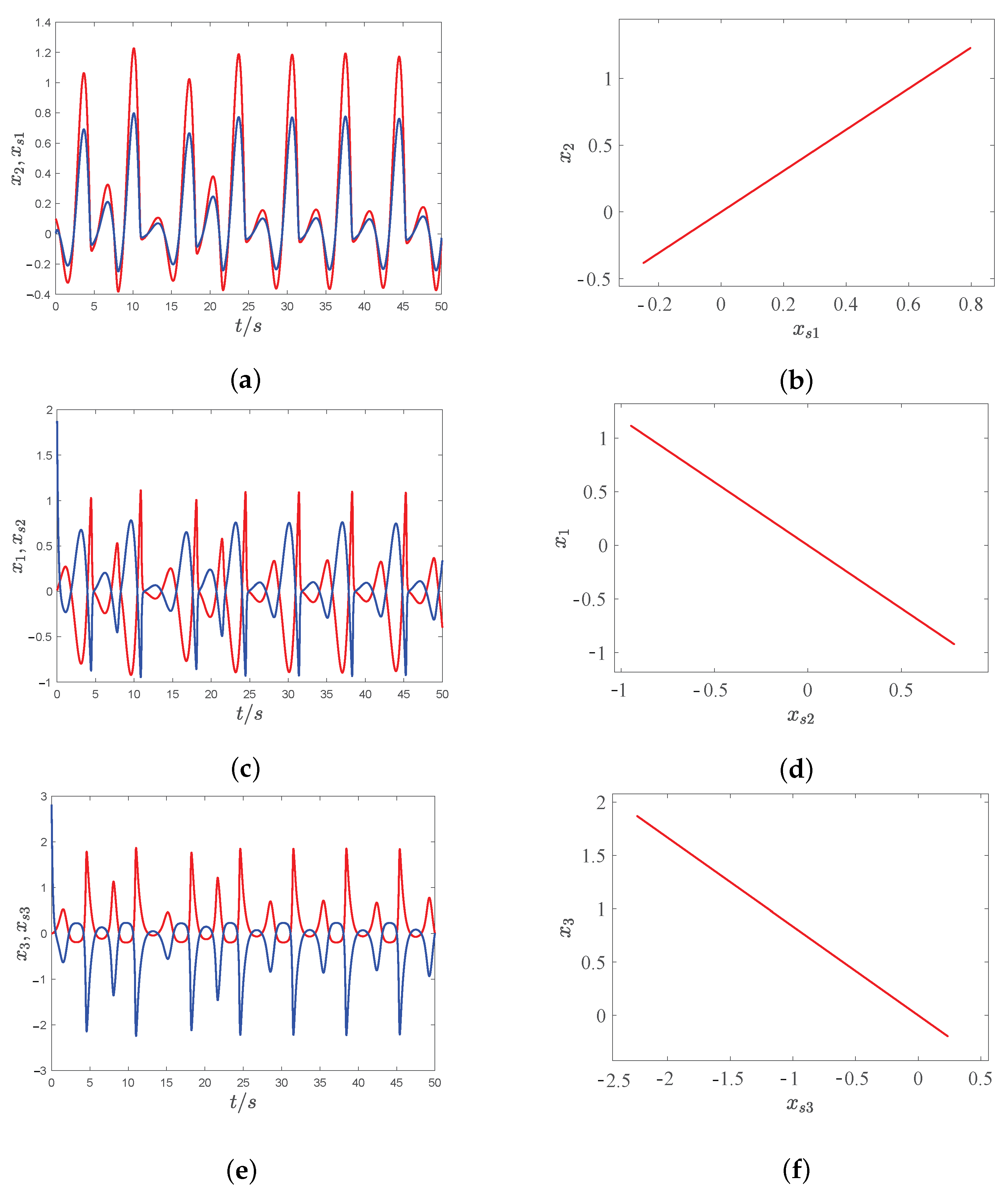
5.2. Numerical Simulation of Misalignment Projection Synchronization

In the numerical simulation of misalignment projection synchronization of the system, the system parameters are a = 1 , b = 4 and q = 0.45 , respectively. The internal parameters of memristor α = 1 , β = 1 . The initial values of the fractional slave system are (0.01, 0.1, 0), and the initial values of the master system are (2, 3, 1). Further selection of the matrix Φ is shown below
Φ = α 11 α 12 α 13 α 21 α 22 α 23 α 31 α 32 α 33 = 0 0.65 0 0.85 0 0 0 0 1.2
Therefore, the synchronization error of the system’s misalignment projection is
e 1 = x s 1 0.85 x 2 e 2 = x s 2 + 0.65 x 1 e 3 = x s 3 1.2 x 3
The numerical simulation results of the system’s misalignment projection synchronization are shown in Figure 15. From Equation (31), it can be seen that variables x s 1 , x s 2 and x s 3 are synchronized with 0.85 x 2 , 0.65 x 1 and 1.2 x 4 , respectively. The curves of the sequence diagram x s 1 , x 2 , x s 2 , x 1 and x s 3 , x 3 are shown in Figure 15a,c,e. The corresponding synchronization phase diagram curves are shown in Figure 15b,d,f. After numerical simulation, it was found that the fractional-order system achieved misalignment projection synchronization.

6. Conclusions

In this paper, the circuit model of a fractional-order 3D flux-controlled memristor is obtained through the theoretical analysis of fractional-order Caputo definition, which shows the rationality of the establishment of this memristor. Subsequently, a memristor is incorporated to develop a fractional-order chaotic system, composed solely of resistance, inductance and capacitance elements. The system’s phase diagram and Poincaré section are then analyzed using the Adomian decomposition algorithm. Meanwhile, the bifurcation diagram and LEs with fractional order q, system parameter a and memristor internal parameter α as variables are found to have the coexistence of up and down symmetric bifurcation path dynamics. Specifically, there are period-doubling bifurcations, reverse-period-doubling bifurcations, and special chaotic degradation phenomena on the bifurcation path. Secondly, for the complexity of the system, under the comparative study of the C 0 algorithm and SE algorithm, it was found that the C 0 algorithm portrays the dynamic behavior of the system more accurately. Finally, based on the fractional-order generalized projection synchronization theory, a fractional-order misaligned projection synchronization scheme is proposed for the system. The viability of this proposed scheme is further substantiated through both theoretical analysis and numerical simulations. Using the chaotic time series of fractional-order system misalignment projection synchronization for secure communication, image encryption, and the parallel computing of Hash Values in plaintext, images will have higher security and can effectively resist known-plaintext attacks. In light of this, the generalized misalignment correction projection synchronization of chaotic systems discussed in this paper has significant practical value.

Author Contributions

J.L.: Conceptualization; Methodology; Writing—Original Draft; and Writing—Review and Editing. H.T.: Formal Analysis; Software. Z.W.: Supervision; Funding Acquisition. Y.G.: Resources; Supervision. Z.C.: Investigation; Validation. All authors have read and agreed to the published version of the manuscript.

Funding

The author acknowledges the referees and the editor for carefully reading this paper and giving many helpful comments. This work is supported by the Natural Science Basic Research Program of Shaanxi (2022JM-029), the Scientific Research Program Funded by the Education Department of Shaanxi Provincial Government (23JK0706), the Scientific Research Foundation of Xijing University (XJ21B01), and the Scientific Research Foundation of Xijing University (XJ230108). The authors also express their gratitude to the reviewers for their insightful comments.

Data Availability Statement

Data are contained within the article.

Acknowledgments

The author acknowledges the referees and the editor for carefully reading this paper and giving many helpful comments. The authors also express their gratitude to the reviewers for their insightful comments.

Conflicts of Interest

The authors declare no conflict of interest.

Appendix A

The decomposition processes of the nonlinear terms x 1 x 3 2 , x 1 x 3 3 , and x 1 x 3 in system (8) are shown in Equations (A1)–(A3), respectively.
A 0 = x 1 0 x 3 0 2 A 1 = x 1 1 x 3 0 2 + 2 x 1 0 x 3 0 x 3 1 A 2 = x 1 2 x 3 0 2 + 2 x 1 1 x 3 0 x 3 1 + 2 x 1 0 x 3 0 x 3 2 + x 1 0 x 3 1 2 A 3 = x 1 3 x 3 0 2 + 2 x 1 2 x 3 0 x 3 1 + 2 x 1 1 x 3 0 x 3 2 + x 1 1 x 3 1 2 + 2 x 1 0 x 3 0 x 3 3 + 2 x 1 0 x 3 1 x 3 2 A 4 = x 1 4 x 3 0 2 + 2 x 1 3 x 3 0 x 3 1 + 2 x 1 2 x 3 0 x 3 2 + x 1 2 x 3 1 2 + 2 x 1 1 x 3 0 x 3 3 + 2 x 1 1 x 3 1 x 3 2 + 2 x 1 0 x 3 0 x 3 4 + 2 x 1 0 x 3 1 x 3 3 + x 1 0 x 3 2 2
A 0 = x 1 0 x 3 0 3 A 1 = x 1 1 x 3 0 3 + 3 x 1 0 x 3 0 2 x 3 1 A 2 = x 1 2 x 3 0 3 + 6 x 1 1 x 3 0 2 x 3 1 + 6 x 1 0 x 3 0 x 3 1 2 + 3 x 1 0 x 3 0 2 x 3 2 A 3 = x 1 3 x 3 0 3 + 3 x 1 2 x 3 0 2 x 3 1 + 6 x 1 2 x 3 0 2 x 3 1 + 18 x 1 1 x 3 0 x 3 1 2 + 9 x 1 1 x 3 0 2 x 3 2 + 6 x 1 0 x 3 1 3 + 18 x 1 0 x 3 0 x 3 1 x 3 2 + 6 x 1 0 x 3 0 2 x 3 3 A 4 = x 1 4 x 3 0 3 + 3 x 1 3 x 3 0 2 x 3 1 + 9 x 1 3 x 3 0 2 x 3 1 + 36 x 1 2 x 3 0 x 3 1 2 + 18 x 1 2 x 3 0 2 x 3 2 + 24 x 1 1 x 3 1 3 + 72 x 1 1 x 1 0 x 3 1 x 3 2 + 9 x 1 1 x 3 0 2 x 3 3 + 36 x 1 0 x 3 1 2 x 3 2 + 18 x 1 0 x 3 0 x 3 2 x 3 2 + 30 x 1 0 x 3 0 x 3 1 x 3 3 + 6 x 1 1 x 3 0 2 x 3 3 + 6 x 1 0 x 3 0 2 x 3 4
A 0 = x 1 0 x 3 0 A 1 = x 1 1 x 3 0 + x 1 0 x 3 1 A 2 = x 1 2 x 3 0 + x 1 1 x 3 1 + x 1 0 x 3 2 A 3 = x 1 3 x 3 0 + x 1 2 x 3 1 + x 1 2 x 3 2 + x 1 0 x 3 3 A 4 = x 1 4 x 3 0 + x 1 2 x 3 2 + x 1 3 x 3 1 + x 1 2 x 3 3 + x 1 0 x 3 4

Appendix B

The iteration coefficients for the numerical solution of the system are as follows
c 1 1 = c 2 0 α c 1 0 ( c 3 0 ) 2 + β c 1 0 ( c 3 0 ) 3 + c 1 0 c 2 1 = c 1 0 0.4 c 2 0 c 3 1 = c 1 0 a c 3 0 + b c 1 0 c 3 0 c 1 2 = c 2 1 α ( c 1 1 c 3 0 c 3 0 + 2 c 1 0 c 3 1 c 3 0 ) + β ( c 1 1 ( c 3 0 ) 3 + 3 c 1 0 c 3 1 ( c 3 0 ) 2 ) + c 1 1 c 2 2 = c 1 1 0.4 c 2 1 c 3 2 = c 1 1 a c 3 1 + b ( c 1 1 c 3 0 + c 1 0 c 3 1 ) c 1 3 = c 2 2 α ( c 1 2 c 3 0 c 3 0 + 2 c 1 0 c 3 2 c 3 0 + ( 2 c 1 1 c 3 1 c 3 0 + c 1 0 c 3 1 c 3 1 ) Γ 2 q + 1 Γ 2 q + 1 + β ( c 1 2 ( c 3 0 ) 3 + ( 3 c 1 0 c 3 2 ( c 3 0 ) 2 + ( 3 c 1 1 c 3 1 ( c 3 0 ) 2 + 3 c 1 0 c 3 1 c 3 1 c 3 0 ) Γ 2 q + 1 Γ 2 q + 1 ) + c 1 2 c 2 3 = c 1 2 0.4 c 2 2 c 3 3 = c 1 2 a c 3 2 + b ( c 1 2 c 3 0 + c 1 0 c 3 2 + c 1 1 c 3 1 Γ 2 q + 1 Γ 2 q + 1 ) c 1 4 = c 2 3 α ( c 1 3 c 3 0 c 3 0 + 2 c 1 0 c 3 3 c 3 0 + 2 ( c 1 2 c 3 1 c 3 0 + c 1 1 c 3 2 c 3 0 + c 1 0 c 3 2 c 3 1 ) Γ 3 q + 1 Γ q + 1 Γ 2 q + 1 + c 1 1 c 3 1 c 3 1 Γ 3 q + 1 Γ 3 q + 1 ) + β ( c 1 3 ( c 3 0 ) 3 + ( 3 c 1 0 c 3 3 ( c 3 0 ) 2 + 3 c 1 2 c 3 1 ( c 3 0 ) 2 + 3 c 1 1 c 3 2 ( c 3 0 ) 2 + 6 c 1 0 c 3 2 c 3 1 c 3 0 ) Γ 3 q + 1 Γ q + 1 Γ 2 q + 1 ) + ( 9 / 2 c 1 1 c 3 1 c 3 1 c 3 0 + 3 / 2 c 1 0 ( c 3 1 ) 3 ) Γ 3 q + 1 Γ 3 q + 1 ) + c 1 3 c 2 4 = c 1 3 0.4 c 2 3 c 3 4 = c 1 3 a c 3 3 + b ( c 1 3 c 3 0 + c 1 0 c 3 3 + ( c 1 2 c 3 1 + c 1 1 c 3 2 ) Γ 3 q + 1 Γ q + 1 Γ 2 q + 1 ) c 1 5 = c 2 4 α ( c 1 4 c 3 0 c 3 0 + 2 c 1 0 c 3 4 c 3 0 + 2 ( c 1 3 c 3 1 c 3 0 + c 1 1 c 3 3 c 3 0 + c 1 0 c 3 3 c 3 1 ) Γ 4 q + 1 Γ q + 1 Γ 3 q + 1 + ( 2 c 1 1 c 3 1 c 3 2 + c 1 2 c 3 1 c 3 1 ) Γ 4 q + 1 Γ 2 q + 1 Γ 2 q + 1 + ( c 1 0 c 3 2 c 3 2 + 2 c 1 2 c 3 0 c 3 2 ) Γ 4 q + 1 Γ 2 2 q + 1 ) + β ( c 1 4 ( c 3 0 ) 3 + ( 3 c 1 3 c 1 1 ( c 3 0 ) 2 + 3 c 1 1 c 3 3 ( c 3 0 ) 2 + 6 c 1 0 c 3 3 c 3 1 c 3 0 ) Γ 4 q + 1 Γ q + 1 Γ 3 q + 1 + ( 3 c 1 2 c 3 2 ( c 3 0 ) 2 + 3 c 1 0 c 3 2 c 3 2 c 3 0 ) Γ 4 q + 1 Γ 2 2 q + 1 + ( 21 / 2 c 1 2 c 3 1 c 3 1 c 3 0 + 21 / 2 c 1 1 c 3 2 c 3 1 c 3 0 + 21 / 4 c 1 0 c 3 2 ( c 3 1 ) 2 ) Γ 4 q + 1 Γ 2 q + 1 Γ 2 q + 1 + 3 c 1 1 ( c 3 1 ) 3 Γ 4 q + 1 Γ 4 q + 1 + 3 c 1 0 c 3 4 ( c 3 0 ) 2 ) + c 1 4 c 2 5 = c 1 4 0.4 c 2 4 c 3 5 = c 1 4 a c 3 4 + b ( c 1 4 c 3 0 + c 1 0 c 3 4 + ( c 1 3 c 3 1 + c 1 1 c 3 3 ) Γ 4 q + 1 Γ q + 1 Γ 3 q + 1 + c 1 2 c 3 2 Γ 4 q + 1 Γ 2 2 q + 1 )

References

  1. Chua, L. Memristor-the missing circuit element. IEEE Trans. Circuit Theory 1971, 18, 507–519. [Google Scholar] [CrossRef]
  2. Chua, L.O.; Kang, S.M. Memristive devices and systems. Proc. IEEE 1976, 64, 209–223. [Google Scholar] [CrossRef]
  3. Strukov, D.B.; Snider, G.S.; Stewart, D.R.; Williams, R.S. The missing memristor found. Nature 2008, 453, 80–83. [Google Scholar] [CrossRef] [PubMed]
  4. Mao, J.-Y.; Zhou, L.; Zhu, X.; Zhou, Y.; Han, S.-T. Photonic memristor for future computing: A perspective. Adv. Opt. Mater. 2019, 7, 1900766. [Google Scholar] [CrossRef]
  5. Ghosh, P.K.; Riam, S.Z.; Ahmed, M.S.; Sundaravadivel, P. CMOS-Based Memristor Emulator Circuits for Low-Power Edge-Computing Applications. Electronics 2023, 12, 1654. [Google Scholar] [CrossRef]
  6. Li, C.; Yang, Y.; Yang, X.; Zi, X.; Xiao, F. A tristable locally active memristor and its application in Hopfield neural network. Nonlinear Dyn. 2022, 108, 1697–1717. [Google Scholar] [CrossRef]
  7. Cao, Z.; Sun, B.; Zhou, G.; Mao, S.; Zhu, S.; Zhang, J.; Ke, C.; Zhao, Y.; Shao, J. Memristor-based neural networks: A bridge from device to artificial intelligence. Nanoscale Horiz. 2023, 8, 716–745. [Google Scholar] [CrossRef]
  8. Danilin, S.N.; Shchanikov, S.A.; Galushkin, A.I. The research of memristor-based neural network components operation accuracy in control and communication systems. In Proceedings of the 2015 International Siberian Conference on Control and Communications (SIBCON), Omsk, Russia, 21–23 May 2015; pp. 1–6. [Google Scholar]
  9. Hasan, G. Real-time fuzzy-pid synchronization of memristor-based chaotic circuit using graphical coded algorithm in secure communication applications. Phys. Scr. 2022, 97, 055212. [Google Scholar]
  10. Luigi, F.; Arturo, B. Spiking neuron mathematical models: A compact overview. Bioengineering 2023, 10, 174. [Google Scholar]
  11. Mikhail, K.; Nikolay, N.; Iveta, N.; Irina, N.; Velika, K.; Marian, M. On a Mathematical Model of a General Autoimmune Disease. Axioms 2023, 12, 1021. [Google Scholar]
  12. Ella, G. TiO2-based memristors and ReRAM: Materials, mechanisms and models (a review). Semicond. Sci. Technol. 2014, 29, 104004. [Google Scholar]
  13. Mao, S.; Sun, B.; Ke, C.; Qin, J.; Yang, Y.; Guo, T.; Wu, Y.A.; Shao, J.; Zhao, Y. Evolution between CRS and NRS behaviors in MnO2@ TiO2 nanocomposite based memristor for multi-factors-regulated memory applications. Nano Energy 2023, 107, 108117. [Google Scholar] [CrossRef]
  14. Sun, K.; Chen, J.; Yan, X. The future of memristors: Materials engineering and neural networks. Adv. Funct. Mater. 2021, 31, 2006773. [Google Scholar] [CrossRef]
  15. Di Ventra, M.; Pershin, Y.V.; Chua, L.O. Circuit elements with memory: Memristors, memcapacitors, and meminductors. Proc. IEEE 2009, 97, 1717–1724. [Google Scholar] [CrossRef]
  16. Petráš, I.; Chen, Y.; Coopmans, C. Fractional-order memristive systems. In Proceedings of the 2009 IEEE Conference on Emerging Technologies & Factory Automation, Palma de Mallorca, Spain, 22–25 September 2009; pp. 1–8. [Google Scholar]
  17. Fouda, M.E.; Radwan, A.G. On the fractional-order memristor model. J. Fract. Calc. Appl. 2013, 4, 1–7. [Google Scholar]
  18. Fouda, M.E.; Radwan, A.G. Fractional-order memristor response under DC and periodic signals. Circuits Syst. Signal Process. 2015, 34, 961–970. [Google Scholar] [CrossRef]
  19. Ding, D.; Li, S.; Wang, N. Dynamics analysis of fractional-order memristive chaotic system. J. Harbin Inst. Technol. (New Ser.) 2020, 27, 65–74. [Google Scholar]
  20. Qin, C.; Sun, K.; He, S. Characteristic analysis of fractional-order memristor-based hypogenetic jerk system and its DSP implementation. Electronics 2021, 10, 841. [Google Scholar] [CrossRef]
  21. Tian, H.; Liu, J.; Wang, Z.; Xie, F.; Cao, Z. Characteristic analysis and circuit implementation of a novel fractional-order memristor-based clamping voltage drift. Fractal Fract. 2022, 7, 2. [Google Scholar] [CrossRef]
  22. Liu, J.; Wang, Z.; Chen, M.; Zhang, P.; Yang, R.; Yang, B. Chaotic system dynamics analysis and synchronization circuit realization of fractional-order memristor. Eur. Phys. J. Spec. Top. 2022, 231, 3095–3107. [Google Scholar] [CrossRef]
  23. Akgül, A.; Rajagopal, K.; Durdu, A.; Pala, M.A.; Boyraz, Ö.F.; Yildiz, M.Z. A simple fractional-order chaotic system based on memristor and memcapacitor and its synchronization application. Chaos Solitons Fractals 2021, 152, 111306. [Google Scholar] [CrossRef]
  24. Wang, Z.; Tian, H.; Krejcar, O.; Namazi, H. Synchronization in a network of map-based neurons with memristive synapse. Eur. Phys. J. Spec. Top. 2022, 231, 4057–4064. [Google Scholar] [CrossRef]
  25. Chang, H.; Li, Y.; Chen, G.; Yuan, F. Extreme multistability and complex dynamics of a memristor-based chaotic system. Int. J. Bifurc. Chaos 2020, 30, 2030019. [Google Scholar] [CrossRef]
  26. Chen, M.; Sun, M.; Bao, B.; Wu, H.; Xu, Q.; Wang, J. Controlling extreme multistability of memristor emulator-based dynamical circuit in flux–charge domain. Nonlinear Dyn. 2018, 91, 1395–1412. [Google Scholar] [CrossRef]
  27. Fatemeh, P.; Sajad, J.; Hamed, A. Traveling patterns in a network of memristor-based oscillators with extreme multistability. Eur. Phys. J. Spec. Top. 2019, 228, 2123–2131. [Google Scholar]
  28. Pecora, L.M.; Carroll, T.L. Synchronization in chaotic systems. Phys. Rev. Lett. 1990, 64, 821. [Google Scholar] [CrossRef]
  29. Chen, W.-H.; Wang, Z.; Lu, X. On sampled-data control for master-slave synchronization of chaotic Lur’e systems. IEEE Trans. Circuits Syst. II Express Briefs 2012, 59, 515–519. [Google Scholar] [CrossRef]
  30. Tian, H.; Wang, Z.; Zhang, H.; Cao, Z.; Zhang, P. Dynamical analysis and fixed-time synchronization of a chaotic system with hidden attractor and a line equilibrium. Eur. Phys. J. Spec. Top. 2022, 231, 2455–2466. [Google Scholar] [CrossRef]
  31. Abarbanel, H.D.I.; Rulkov, N.F.; Sushchik, M.M. Generalized synchronization of chaos: The auxiliary system approach. Phys. Rev. E 1996, 53, 4528. [Google Scholar] [CrossRef]
  32. Bernd, B.; Lewi, S. Chaos and phase synchronization in ecological systems. Int. J. Bifurc. Chaos 2000, 10, 2361–2380. [Google Scholar]
  33. Min, F.; Wang, E. Misalignment projection synchronization of hyperchaotic Qi systems and its application in secure communication. Acta Phys. Sin. 2010, 59, 7657–7662. [Google Scholar]
  34. Sun, J.; Wang, Y.; Yao, L.; Shen, Y.; Cui, G. General hybrid projective complete dislocated synchronization between a class of chaotic real nonlinear systems and a class of chaotic complex nonlinear systems. Appl. Math. Model. 2015, 39, 6150–6164. [Google Scholar] [CrossRef]
  35. Li, D. Modified functional projective synchronization of the unidirectional and bidirectional hybrid connective star network with coupling time-delay. Wuhan Univ. J. Nat. Sci. 2019, 24, 321–328. [Google Scholar] [CrossRef]
  36. Li, C.-L.; Li, Z.-Y.; Feng, W.; Tong, Y.-N.; Du, J.-R.; Wei, D.-Q. Dynamical behavior and image encryption application of a memristor-based circuit system. AEU-Int. J. Electron. Commun. 2019, 110, 152861. [Google Scholar] [CrossRef]
  37. Ivo, P. Fractional-Order Nonlinear Systems: Modeling, Analysis and Simulation; Springer Science & Business Media: Berlin/Heidelberg, Germany, 2011. [Google Scholar]
  38. Marian, M.; Stoyan, Z. A note about stability of fractional retarded linear systems with distributed delays. Int. J. Pure Appl. Math. 2017, 115, 873–881. [Google Scholar]
  39. Hristo, K.; Mariyan, M.; Magdalena, V.; Andrey, Z. Continuous Dependence on the Initial Functions and Stability Properties in Hyers–Ulam–Rassias Sense for Neutral Fractional Systems with Distributed Delays. Fractal Fract. 2023, 7, 742. [Google Scholar]
  40. Cherruault, Y.; Adomian, G. Decomposition methods: A new proof of convergence. Math. Comput. Model. 1993, 18, 103–106. [Google Scholar] [CrossRef]
  41. Abdul-Majid, W. A new algorithm for calculating Adomian polynomials for nonlinear operators. Appl. Math. Comput. 2000, 111, 33–51. [Google Scholar]
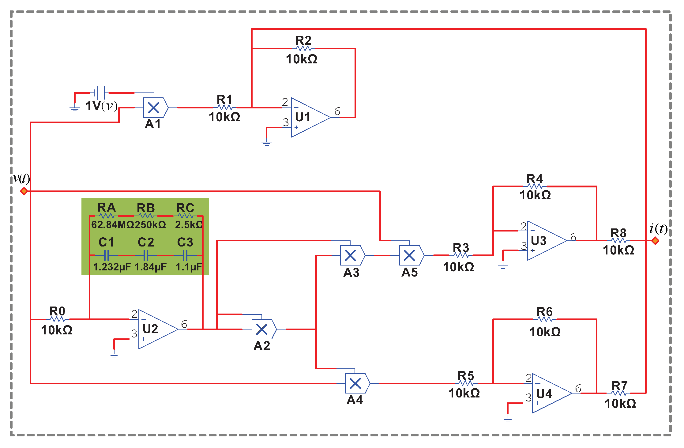
Figure 1. Hysteresis loop area of memristor with different fractional orders q.
Axioms 12 01125 g001
Figure 2. Circuit schematic diagram of fractional-order flux-controlled memristor.
Axioms 12 01125 g002
Figure 3. Simulation results of v t - i t curve of memristor controlled by 3D fractional flux. (a) Analog circuit results; (b) numerical simulation results.
Axioms 12 01125 g003
Figure 4. Circuit system schematic diagram of 3D fractional-order flux-controlled memristor.
Axioms 12 01125 g004
Figure 5. Chaotic attractor diagram of the system. (a) The projection of the chaotic attractor on the plane ( x 1 , x 2 ); (b) the chaotic attractor in the three-dimensional space ( x 1 , x 2 , x 3 ).
Axioms 12 01125 g005
Figure 6. Poincaré section and projection of the system. (a) x 2 = 0 in x 1 - x 3 - x 2 section in three-dimensional space; (b) x 3 = 0 in x 1 - x 2 - x 3 section in three-dimensional space.
Axioms 12 01125 g006
Figure 7. System order q changes. (a) Bifurcation diagram; (b) two LEs greater than zero.
Axioms 12 01125 g007
Figure 8. p-s plane trajectory of the system. (a) q = 0.55 ; (b) q = 0.62 .
Axioms 12 01125 g008
Figure 9. System parameter a changes. (a) Bifurcation diagram; (b) two LEs greater than zero.
Axioms 12 01125 g009
Figure 10. System parameter α changes. (a) Bifurcation diagram; (b) two LEs greater than zero.
Axioms 12 01125 g010
Figure 11. Chaotic degradation dynamic behavior of the system. (a) Time domain waveform of state variable x 1 within time (the blue line represents chaotic state and the red line is periodic state); (b) time domain waveform of state variable x 1 within time t ( 100   s 200   s ); (c) the projection of chaotic attractor in time t ( 0   s 35   s ); (d) stable periodic limit cycle in time t ( 100   s 200   s ).
Axioms 12 01125 g011
Figure 12. The complexity of system fractional order q changes. (a) C 0 complexity; (b) SE complexity.
Axioms 12 01125 g012
Figure 13. The complexity of system internal parameter α changes. (a) C 0 complexity; (b) SE complexity.
Axioms 12 01125 g013
Figure 14. Chaotic map of system structure complexity (dark-red area that exhibits complex chaotic behavior). (a) C 0 complexity chaotic map; (b) SE complexity chaotic map.
Axioms 12 01125 g014
Figure 15. Numerical results of system misalignment projection synchronization. (a) Time series (blue) x s 1 and (red) x 2 ; (b) synchronization phase diagram x s 1 - x 2 ; (c) time series (blue) x s 2 and (red) x 1 ; (d) synchronization phase diagram x s 2 - x 1 ; (e) time series (blue) x s 3 and (red) x 3 ; (f) synchronization phase diagram x s 3 - x 3 .
Axioms 12 01125 g015
Table 1. Circuit parameters of 3D fractional-order flux-controlled memristor.
Circuit ParametersPhysical MeaningParameter Value
C1Capacitance1.232  μ F
C2Capacitance1.84  μ F
C3Capacitance1.1  μ F
R0/R1/R2/R3/R4/R5/R6/R7/R8Resistance10 k Ω
RAResistance62.84 M Ω
RBResistance250 k Ω
RCResistance2.5 k Ω
Disclaimer/Publisher’s Note: The statements, opinions and data contained in all publications are solely those of the individual author(s) and contributor(s) and not of MDPI and/or the editor(s). MDPI and/or the editor(s) disclaim responsibility for any injury to people or property resulting from any ideas, methods, instructions or products referred to in the content.

