Efficiency of Orthogonal Matching Pursuit for Group Sparse Recovery

Abstract

We propose the Group Orthogonal Matching Pursuit (GOMP) algorithm to recover group sparse signals from noisy measurements. Under the group restricted isometry property (GRIP), we prove the instance optimality of the GOMP algorithm for any decomposable approximation norm. Meanwhile, we show the robustness of the GOMP under the measurement error. Compared with the P-norm minimization approach, the GOMP is easier to implement, and the assumption of $\gamma$-decomposability is not required. The simulation results show that the GOMP is very efficient for group sparse signal recovery and significantly outperforms Basis Pursuit in both scalability and solution quality.

1. Introduction

The problem of recovering sparse signals from incomplete measurements has been studied extensively in the field of compressed sensing. Many important results have been obtained, see refs. [1,2,3,4,5]. In this article, we consider the problem of recovering group sparse signals. We first recall some basic notions and results.

Assume that $x\in {\mathbb{R}}^n$ is an unknown signal, and the information we gather about $x\in {\mathbb{R}}^n$ can be described by

$$y=\mathsf{\Phi }x+e,$$

(1)

where $\mathsf{\Phi }\in {\mathbb{R}}^{m\times n}$ is the encoder matrix and $y\in {\mathbb{R}}^m$ is the information vector with a noise level ${\parallel e\parallel }_2\le ϵ$. To recover x from $y,$ we use a decoder $\mathsf{\Delta }$, which is a mapping from ${\mathbb{R}}^m$ to ${\mathbb{R}}^n$, and denote

$$x^{*}:=\mathsf{\Delta }\left(y\right)=\mathsf{\Delta }(\mathsf{\Phi }x+e)$$

as our approximation of $x.$

The $l_1$-norm minimization, also known as Basis Pursuit [2], is one of the most popular decoder maps. It is defined as follows:

$${\mathsf{\Delta }}_{\mathrm{BP}}\left(y\right):={\arg \min }_{z\in {\mathbb{R}}^n}{\parallel z\parallel }_1,\mathrm{s}.\mathrm{t}.{\parallel y-\mathsf{\Phi }z\parallel }_2\le ϵ.$$

(2)

Candès and Tao in Ref. [6] introduced the restricted isometry property (RIP) of a measurement matrix as follows:

A matrix $\mathsf{\Phi }$ is said to satisfy the RIP of order k if there exists a constant $\delta \in (0,1)$ such that, for all k-sparse signals $x,$

$${(1-\delta )\parallel x\parallel }_2^2\le {\parallel \mathsf{\Phi }x\parallel }_2\le (1+\delta ){\parallel x\parallel }_2^2.$$

In particular, the minimum of all $\delta$ satisfying the above inequality is defined as the isometry constant ${\delta }_k.$

Based on the RIP of the encoder matrix $\mathsf{\Phi },$ it has been shown that the solution to (2) recovers x exactly provided that x is sufficiently sparse [7]. We denote by ${\mathsf{\Sigma }}_k$ the set of all k-sparse signals, i.e.,

$${\mathsf{\Sigma }}_k:=\{z\in {\mathbb{R}}^n:\left|\mathit{supp}\left(z\right)\right|\le k\},$$

where $\mathit{supp}\left(z\right)$ is the set of i for which $z_i\ne 0$ and $\left|A\right|$ is the cardinality of the set $A.$ Let ${\sigma }_k{(x,\parallel ·\parallel }_1)$ be the sparsity index of x from ${\mathsf{\Sigma }}_k,$ which is defined by

$${\sigma }_k{(x,\parallel ·\parallel }_1):=\underset{z\in {\mathsf{\Sigma }}_k}{inf}{\parallel x-z\parallel }_1.$$

In Ref. [7], the authors obtained the estimation of the residual error

$${\parallel {\mathsf{\Delta }}_{\mathrm{BP}}\left(y\right)-x\parallel }_2\le \frac{C_0}{\sqrt{k}}{\sigma }_k{(x,\parallel ·\parallel }_1)+C_1ϵ,$$

(3)

where $C_0,C_1$ are constants depending only on the encoder matrix $\mathsf{\Phi }$ but not on x or e. In many current papers on sparse recovery, the $l_1$-norm objective function in (2) has been changed to several other norms.

At about the same time, the research community began to propose that the number of nonzero components of a signal might not be the only reasonable measure of the sparsity of a signal. Alternate notions under the broad umbrella of “group sparsity” and “group sparse recovery” began to appear. For more detail, one can see Ref. [8]. It has been shown that group sparse signals are used widely in EEG [9], wavelet image analysis [10], gene analysis [11], multi-channel image analysis [12] and other fields.

We next recall a result on the recovering of the group sparse signals from Ref. [13]. In that paper, Ahsen and Vidyasagar estimated x from y by solving the following optimization problem:

$${\mathsf{\Delta }}_P\left(y\right):={\arg \min }_{z\in {\mathbb{R}}^n}{\parallel z\parallel }_P,\mathrm{s}.\mathrm{t}.{\parallel y-\mathsf{\Phi }z\parallel }_2\le ϵ,$$

(4)

where ${\parallel ·\parallel }_P$ is the penalty norm. We begin with recalling some definitions from [13]. We denote the set $\{1,2,\dots ,n\}$ by the symbol $\left[n\right].$ The group structure $\mathcal{G}=\{G_1,G_2,\dots ,G_g\}$ is a partition of $\left[n\right].$ Here, we suppose that $|G_i|\le k$ for all $1\le i\le g.$ A signal $x\in {\mathbb{R}}^n$ is said to be group k-sparse if its support set supp(x) is contained in a group k-sparse set, which is defined as follows:

Definition 1.

A subset $\mathsf{\Lambda }\subseteq \left[n\right]$ is said to be group k-sparse if $\mathsf{\Lambda }=G_S:={\cup }_{i\in S}{G}_i$ for some $S\subseteq \{1,2,\dots ,g\}$ and $\left|\mathsf{\Lambda }\right|\le k.$

We use GkS to denote the set of all group k-sparse subsets of $\left[n\right].$

Definition 2.

We say a norm $\parallel ·\parallel$ on ${\mathbb{R}}^n$ is decomposable if $x,y\in {\mathbb{R}}^n,$ satisfy $\mathit{supp}\left(x\right)\subseteq G_S,\mathit{supp}\left(y\right)\subseteq G_T,$ with $S,T$ being disjoint subsets of $\{1,2,\dots ,g\},$ then one has $\parallel x+y\parallel =\parallel x\parallel +\parallel y\parallel .$

It is clear that $l_1$-norm is decomposable. More examples of decomposable norms can be found in Ref. [13].

In the processing of recovering an unknown signal $x\in {\mathbb{R}}^n,$ the approximation norm on ${\mathbb{R}}^n$ will be denoted by ${\parallel ·\parallel }_A.$ We assume that the approximation norm is decomposable.

Definition 3.

If there exists $\gamma \in (0,1]$ such that for any $x,y\in {\mathbb{R}}^n$ with $\mathit{supp}\left(x\right)\subseteq G_S,\mathit{supp}\left(y\right)\subseteq G_T,$ and $S,T$ are disjoint subsets of $\{1,2,\dots ,g\},$ it is true that $\parallel x+y\parallel \ge \parallel x\parallel +\gamma \parallel y\parallel ,$ we say the norm $\parallel ·\parallel$ is γ-decomposable.

Note that when $\gamma =1$, $\gamma$-decomposability coincides with decomposability.

For any index set $A\subseteq \left[n\right],$ let $x_A$ denote the part of the signal x consisting of coordinates falling on $A.$ The sparsity index and the optimal decomposition of a signal in ${\mathbb{R}}^n$ are defined respectively as follows:

Definition 4.

The group k-sparse index of a signal $x\in {\mathbb{R}}^n$ with respect to the norm $\parallel ·\parallel$ and the group structure $\mathcal{G}$ is defined by

$${\sigma }_{k,\mathcal{G}}(x,\parallel ·\parallel ):=\underset{\mathsf{\Lambda }\in \mathrm{GkS}}{min}\parallel x-x_{\mathsf{\Lambda }}\parallel =\underset{\mathsf{\Lambda }\in \mathrm{GkS}}{min}\parallel x_{{\mathsf{\Lambda }}^c}\parallel .$$

For $x\in {\mathbb{R}}^n$ and a norm $\parallel ·\parallel$ on ${\mathbb{R}}^n,$ if there exist ${\mathsf{\Lambda }}_i\in \mathrm{GkS}$ for $i=0,1,2,\dots ,s,$ such that

$$\parallel x_{{\mathsf{\Lambda }}_0^c}\parallel =\parallel x-x_{{\mathsf{\Lambda }}_0}\parallel =\underset{\mathsf{\Lambda }\in \mathrm{GkS}}{min}\parallel x-x_{\mathsf{\Lambda }}\parallel ={\sigma }_{k,\mathcal{G}}\left(x\right)$$

and

$$\parallel x_{{\mathsf{\Lambda }}_i^c}\parallel =\underset{\mathsf{\Lambda }\in \mathrm{GkS}}{min}\parallel x-\sum _{j=0}^{i-1}{x}_{{\mathsf{\Lambda }}_j}-x_{\mathsf{\Lambda }}\parallel ,i=1,2,\dots ,s,$$

then we call $\{x_{{\mathsf{\Lambda }}_0},x_{{\mathsf{\Lambda }}_1},\dots ,x_{{\mathsf{\Lambda }}_s}\}$ an optimal group k-sparse decomposition of $x.$

Definition 5.

A matrix $\mathsf{\Phi }\in {\mathbb{R}}^{m\times n}$ is said to satisfy the group restricted isometry property (GRIP) of order k if there exists a constant ${\delta }_k\in (0,1)$, such that

$$1-{\delta }_k\le \underset{\mathsf{\Lambda }\in \mathit{GkS}}{min}\underset{\mathit{supp}\left(z\right)\subseteq \mathsf{\Lambda }}{min}\frac{{\parallel \mathsf{\Phi }z\parallel }_2^2}{{\parallel z\parallel }_2^2}\le \underset{\mathsf{\Lambda }\in \mathit{GkS}}{max}\underset{\mathit{supp}\left(z\right)\subseteq \mathsf{\Lambda }}{max}\frac{{\parallel \mathsf{\Phi }z\parallel }_2^2}{{\parallel z\parallel }_2^2}\le 1+{\delta }_k.$$

Then, we are ready to state the result of Ahsen and Vidyasagar. We need the following constants:

$$a:=\underset{\mathsf{\Lambda }\in \mathrm{GkS}}{min}\underset{x_{\mathsf{\Lambda }}\ne 0}{min}\frac{\parallel x_{\mathsf{\Lambda }}{\parallel }_P}{\parallel x_{\mathsf{\Lambda }}{\parallel }_A},b:=\underset{\mathsf{\Lambda }\in \mathrm{GkS}}{max}\underset{x_{\mathsf{\Lambda }}\ne 0}{max}\frac{\parallel x_{\mathsf{\Lambda }}{\parallel }_P}{\parallel x_{\mathsf{\Lambda }}{\parallel }_A},f:=\sqrt{k}$$

and

$$c:=\underset{\mathsf{\Lambda }\in \mathrm{GkS}}{min}\underset{x_{\mathsf{\Lambda }}\ne 0}{min}\frac{\parallel x_{\mathsf{\Lambda }}{\parallel }_A}{\parallel x_{\mathsf{\Lambda }}{\parallel }_2},d:=\underset{\mathsf{\Lambda }\in \mathrm{GkS}}{max}\underset{x_{\mathsf{\Lambda }}\ne 0}{max}\frac{\parallel x_{\mathsf{\Lambda }}{\parallel }_A}{\parallel x_{\mathsf{\Lambda }}{\parallel }_2}.$$

(5)

Theorem 1.

Suppose that

1. The norm ${\parallel ·\parallel }_A$ is decomposable.

2. The norm ${\parallel ·\parallel }_P$ is γ-decomposable for some $\gamma \in (0,1].$

3. The matrix Φ satisfies GRIP of order $2k$ with constant ${\delta }_{2k}.$

4. Suppose the “compressibility condition"

$${\delta }_{2k}<\frac{fa\gamma /bd}{\sqrt{2}+fa\gamma /bd}$$

holds, then

$$\parallel {\mathsf{\Delta }}_P{(\mathsf{\Phi }x+e)-x\parallel }_2\le D_1{\sigma }_{k,\mathcal{G}}{\left(x\right)}_A+D_2ϵ.$$

Furthermore,

$$\parallel {\mathsf{\Delta }}_P{(\mathsf{\Phi }x+e)-x\parallel }_A\le D_3{\sigma }_{k,\mathcal{G}}{\left(x\right)}_A+D_4ϵ,$$

where

$$D_1=\frac{b(1+\gamma )}{a\gamma f}·\frac{1+(\sqrt{2}-1){\delta }_{2k}}{1-(1+\sqrt{2}bd/a\gamma f){\delta }_{2k}},D_2=2(1+bd/a\gamma f)·\frac{\sqrt{1+{\delta }_{2k}}}{1-(1+\sqrt{2}bd/a\gamma f){\delta }_{2k}}$$

and

$$D_3=\frac{b(1+\gamma )}{a\gamma }·\frac{1+(\sqrt{2}d/f-1){\delta }_{2k}}{1-(1+\sqrt{2}bd/a\gamma f){\delta }_{2k}},D_4=2(1+bd/a\gamma )·\frac{\sqrt{1+{\delta }_{2k}}}{1-(1+\sqrt{2}bd/a\gamma f){\delta }_{2k}}.$$

Recently, Ranjan and Vidyasagar presented sufficient conditions for (2) to achieve robust group sparse recovery by establishing a group robust null space property [14]. They derived the residual error bounds for the $l_p$-norm for $p\in [1,2].$

In compressed sensing, an alternative decoder for (1) is Orthogonal Matching Pursuit (OMP), which was originally proposed by J. Tropp in [15]. It is defined as Algorithm 1:

Algorithm 1 Orthogonal Matching Pursuit (OMP)

Input: measurement matrix $\mathsf{\Phi },$ measurement vector $y.$ Initialization:$S^0=\varnothing ,x^0=0.$ Iteration: repeat until a stopping criterion is met at $n=\overline{n}:$    $S^{n+1}=S^n\cup \left\{j_{n+1}\right\},j_{n+1}:={\arg \max }_{j\in \left[n\right]}{\left\{\right|{\mathsf{\Phi }}^{*}(y-\mathsf{\Phi }{x}^n))}_j\left|\right\},$    $x^{n+1}={\arg \min }_{z\in {\mathbb{R}}^n}{\{\parallel y-\mathsf{\Phi }z\parallel }_2,\mathrm{supp}\left(z\right)\subseteq S^{n+1}\}.$ Output: the $\overline{n}$-sparse vector $x^{\#}=x^{\overline{n}}.$

The major advantage of the OMP algorithm is that it is easy to implement, see Refs. [16,17,18,19,20,21]. In [22], under the RIP, T. Zhang proved that OMP with k iterations can exactly recover k-sparse signals and the procedure is also stable in $l_2$ under measurement noise. Based on this result, Xu showed that the OMP can achieve instance optimality under the RIP, cf. [23]. In [24], Cohen, Dahmen and DeVore extended T. Zhang’s result to the general context of k-term approximation from a dictionary in arbitrary Hilbert spaces. They have shown that OMP generates near-best k-term approximations under a similar RIP condition.

In this article, we will generalize the OMP to recover the group sparse signals. Assume that the signal x is group k-sparse with the group structure $\mathcal{G},$ then the number of non-zero groups of $x=(x_{G_1},x_{G_2},\dots ,x_{G_g})$ is no more than $k.$ We define

$$\alpha :=\underset{j\in \left[g\right]}{max}\left|G_j\right|.$$

It is obvious that $\alpha \le k.$

The group support set of x with respect to $\mathcal{G}$ is defined as follows:

$$\mathrm{Gsupp}\left(x\right):=\{j\in \left[g\right]:x_{G_j}\ne 0\}.$$

Let $\left|\mathrm{Gsupp}\right(x\left)\right|$ be the number of distinct groups on which x is supported. For any $i\in \{1,2,\dots ,g\},$ the subvector (submatrix) $x_{G_i}\left({\mathsf{\Phi }}_{G_i}\right)$ can also be written as $x\left[i\right]\left(\mathsf{\Phi }\right[i\left]\right).$

Now we start to propose the Group Orthogonal Matching Pursuit (GOMP) algorithm. Assume that the group structure $\mathcal{G}$ is given a prior. Let $\mathsf{\Omega }$ be the initial feature set of the group sparse signal x with the maximum allowed sparsity M. The GOMP is defined as Algorithm 2:

Algorithm 2 Group Orthogonal Matching Pursuit (${\mathrm{GOMP}}_M\left(y\right))$

Input: encoding matrix $\mathsf{\Phi },$ the vector $y,$ group structure ${\left\{G_i\right\}}_{i=1}^g,$ a set $\mathsf{\Omega }\subseteq \{1,2,\dots ,g\}$, maximum allowed sparsity M. Initialization:$x^0={\arg \min }_{\tilde{x}:\mathrm{Gsupp}\left(\tilde{x}\right)\subseteq \mathsf{\Omega }}{\parallel y-\mathsf{\Phi }\tilde{x}\parallel }_2$, $r^0=y-\mathsf{\Phi }{x}^0,l=1$, $I_0=\mathsf{\Omega }$.   while$l\le k\le M$do       Set $i_l={\arg \max }_i{\parallel {\mathsf{\Phi }}^{*}\left[i\right]r^{l-1}\parallel }_2$.       Identity $I_l=\{i_1,i_2,\dots ,i_l\}\cup \mathsf{\Omega }.$       Update $x^l={\arg \min }_{\tilde{x}:\mathrm{Gsupp}\left(\tilde{x}\right)\subseteq I_l}{\parallel y-\mathsf{\Phi }\tilde{x}\parallel }_2$, $r^l=y-\mathsf{\Phi }{x}^l$, $l=l+1$.   end while Output: ${\widehat{x}}_{\mathrm{GOMP}}=x^k$.

The GOMP${}_M\left(y\right)$ algorithm begins by initializing the residual as $r^0=y$, and at the lth $(l\ge 1)$ iteration, we chose one group index which matched $r^{l-1}$ best. However, the algorithm does not obtain a least-square minimization over the group index sets that have already been selected, but updates the residual and proceeds to the next iteration.

Then, we studied the efficiency of the GOMP. We show the instance optimality and robustness of the GOMP algorithm under the GRIP of the matrix $\mathsf{\Phi }$. We formulate them in the following theorem.

Theorem 2.

Suppose that the norm ${\parallel ·\parallel }_A$ is decomposable and $0<\delta \le 1.$ If the $\mathit{GRIP}$ condition ${\delta }_{k\alpha }+(1+\delta ){\delta }_{\beta k\alpha }\le \delta$ holds with $\beta :=\lceil 16+15\delta \rceil ,$ then for any signal x and any permutation e with ${\parallel e\parallel }_2\le ϵ,$ the solution $x^{*}:={\mathrm{GOMP}}_{(\beta -1)k}(\mathsf{\Phi }x+e)$ obeys

$$\parallel x^{*}{-x\parallel }_2\le D_1{\sigma }_{k,\mathcal{G}}{\left(x\right)}_A+D_2ϵ,$$

(6)

where

$$D_1=\frac{1}{c}[(1+\delta )(1+\sqrt{11+20\delta })+1]\mathit{and}{D}_2=\sqrt{1+\delta }(1+\sqrt{11+20\delta }).$$

(7)

Furthermore,

$$\parallel x^{*}{-x\parallel }_A\le D_3{\sigma }_{k,\mathcal{G}}{\left(x\right)}_A+D_4ϵ,$$

(8)

where

$$D_3=\frac{d}{c}\sqrt{2\beta \alpha -1}(1+\delta )(1+\sqrt{11+20\delta })+1\mathit{and}{D}_4=d\sqrt{(2\beta \alpha -1)(1+\delta )}(1+\sqrt{11+20\delta }).$$

(9)

When $e=0$, from inequalities (6) and (8), we have

$$\begin{array}{c}\hfill \parallel x^{*}{-x\parallel }_2\le D_1{\sigma }_{k,\mathcal{G}}{\left(x\right)}_A\end{array}$$

and

$$\begin{array}{c}\hfill \parallel x^{*}{-x\parallel }_A\le D_3{\sigma }_{k,\mathcal{G}}{\left(x\right)}_A.\end{array}$$

This implies the instance optimality of the GOMP. In other words, from the viewpoint of the error, the GOMP is almost the best. The robustness of the GOMP means that the signal can be recovered stably for different dimensions, sparsity levels, numbers of measurements and noise scenarios (which can be observed from the experiments in Section 3). Compared with Basis Pursuit (BP), our proposed algorithm performs far better, and runs extremely faster, especially when it comes large-scale problems.

Based on the observation of Theorems 1 and 2, one can see that the assumption of $\gamma$-decomposability is not required for the GOMP. Instead, we developed some new techniques to analyze the error performance of the GOMP.

We remark that the results of Theorem 2 are rather general. They cover some important cases.

Firstly, if $n={\sum }_{i=1}^g{d}_i$ and we take a special partition of $\left[n\right]$ as

$$\left[n\right]=[\underset{G_1}{\underbrace{1,\dots ,d_1}},\underset{G_2}{\underbrace{d_1+1,\dots ,d_1+d_2}},\dots ,\underset{G_g}{\underbrace{n-d_g+1,\dots ,n}}],$$

then the unknown sparse signals appear in a few blocks, i.e., the signals are block-sparse. It is obvious that our results include the case of the block-sparse signals. In practice, there are many forms of block-sparse signal, such as multi-band signal, DNA array, radar pulse signal and the multi-measurement vector problem and so on, see Refs. [25,26,27,28,29,30,31,32].

Secondly, applying Theorem 2 to the case of conventional sparsity, we obtain the following new results on the error estimates of the OMP.

Corollary 1.

(Conventional sparsity) Suppose that Φ satisfies the $\mathit{RIP}$ condition ${\delta }_k+(1+\delta ){\delta }_{\beta k}\le \delta$ with $\beta :=\lceil 16+15\delta \rceil .$ Then,

$$\parallel {\mathrm{OMP}}_{(\beta -1)k}{(\mathsf{\Phi }x+e)-x\parallel }_2\le D_1{\sigma }_k{\left(x\right)}_A+D_2ϵ,$$

and

$$\parallel {\mathrm{OMP}}_{(\beta -1)k}{(\mathsf{\Phi }x+e)-x\parallel }_A\le D_3{\sigma }_k{\left(x\right)}_A+D_4ϵ,$$

where the constants $D_i$ are defined in (1.6) and (1.8) for $i=1,2,3,4.$

The remaining part of the paper is organized as follows. In Section 2, based on a corollary of Theorem 3, we prove Theorem 2, while the proof of Theorem 3 will be given in the Appendix B. In the Appendix A, we establish some preliminary results for the proof. In Section 3, we compare the Group Orthogonal Matching Pursuit (GOMP) with the Basis Pursuit (BP) by numerical experiments. In Section 4, we draw the conclusions of our study. Moreover, we mention some other competitive algorithms which we will study in the future.

2. Proof of Theorem 2

The proof of Theorem 2 is based on the estimation of the residual error of the GOMP algorithm. To establish such estimation, we use the restricted gradient optimal constant for group sparse signals.

Definition 6.

Given $\overline{x}\in {\mathbb{R}}^n$ and $s>0,$ we define the restricted gradient optimal constant ${\epsilon }_s\left(\overline{x}\right)$ as the smallest non-negative value such that

$$|⟨2\mathsf{\Phi }\mu ,\mathsf{\Phi }\overline{x}-y⟩|\le {\epsilon }_s\left(\overline{x}\right){\parallel \mu \parallel }_2$$

for all $\mu \in {\mathbb{R}}^n$ with $\left|\mathrm{Gsupp}\right(\mu \left)\right|\le s.$

Some estimates about ${\epsilon }_s\left(\overline{x}\right)$ have been given in Ref. [22], such as ${\epsilon }_s\left(\overline{x}\right)\le 2\sqrt{s}{\parallel {\mathsf{\Phi }}^{*}(\mathsf{\Phi }\overline{x}-y)\parallel }_{\infty },$ ${\epsilon }_s\left(\overline{x}\right)\le 2{\parallel {\mathsf{\Phi }}^{*}(\mathsf{\Phi }\overline{x}-y)\parallel }_2,$ and so on.

The following theorem is our result of the residual error of the GOMP algorithm. Its proof is quite technical and is given in the Appendix B.

Theorem 3.

Let $\overline{x}\in {\mathbb{R}}^n$ and $\overline{F}=\mathit{Gsupp}\left(\overline{x}\right).$ If there exists s, such that

$$s\ge |\overline{F}\cup \mathsf{\Omega }|+\lceil 4|\overline{F}\backslash \mathsf{\Omega }|\frac{1+{\delta }_{\alpha }}{1-{\delta }_{s\alpha }}ln\frac{20(1+{\delta }_{|\overline{F}\backslash \mathsf{\Omega }|\alpha })}{1-{\delta }_{s\alpha }}\rceil ,$$

(10)

then when $k\ge \lceil 4|\overline{F}\backslash \mathsf{\Omega }|\frac{1+{\delta }_{\alpha }}{1-{\delta }_{s\alpha }}ln\frac{20(1+{\delta }_{|\overline{F}\backslash \mathsf{\Omega }|\alpha })}{1-{\delta }_{s\alpha }}\rceil ,$ we have

$$\parallel \mathsf{\Phi }{x}^k{-y\parallel }_2^2\le {\parallel \mathsf{\Phi }\overline{x}-y\parallel }_2^2+2.5{\epsilon }_s{\left(\overline{x}\right)}^2/(1-{\delta }_{s\alpha }),$$

and

$$\parallel x^k-\overline{x}{\parallel }_2\le \sqrt{6}{\epsilon }_s\left(\overline{x}\right)/(1-{\delta }_{s\alpha }).$$

Next, we will use Theorem 3 in the case of $\mathsf{\Omega }$ being empty to prove the following corollary, which plays an important role in the proof of Theorem 2.

Corollary 2.

Let $\overline{x}\in {\mathbb{R}}^n,\overline{k}=\left|\mathit{Gsupp}\left(\overline{x}\right)\right|.$ Let $0<\delta \le 1,\beta =\lceil 16+15\delta \rceil .$ If the GRIP condition ${\delta }_{\overline{k}\alpha }+(1+\delta ){\delta }_{\beta \overline{k}\alpha }\le \delta$ holds, then for $k=(\beta -1)\overline{k},$ we have

$$\parallel \mathsf{\Phi }{x}^k{-y\parallel }_2^2\le (11+20\delta ){\parallel \mathsf{\Phi }\overline{x}-y\parallel }_2^2.$$

Proof. 

If ${\delta }_{\overline{k}\alpha }+(1+\delta ){\delta }_{\beta \overline{k}\alpha }\le \delta$, then

$$1\le \frac{1+{\delta }_{\alpha }}{1-{\delta }_{\beta \overline{k}\alpha }}\le \frac{1+{\delta }_{\overline{k}\alpha }}{1-{\delta }_{\beta \overline{k}\alpha }}\le 1+\delta .$$

(11)

Therefore, we take $s=\beta \overline{k}$ in (10). Since $0<\delta \le 1,$ then for $k=(\beta -1)\overline{k},$ using the properties of rounding function and logarithm function, we have

$$\begin{array}{cc}\hfill k& \ge \lceil 4\overline{k}(1+\delta )ln\left(20(1+\delta )\right)\rceil \hfill \\ \hfill & \ge \lceil 4\overline{k}\frac{1+{\delta }_{\alpha }}{1-{\delta }_{\beta \overline{k}\alpha }}ln20\frac{1+{\delta }_{\overline{k}\alpha }}{1-{\delta }_{\beta \overline{k}\alpha }}\rceil .\hfill \end{array}$$

From Theorem 3 and inequality (11), we conclude

$$\begin{array}{cc}\hfill \parallel \mathsf{\Phi }{x}^k{-y\parallel }_2^2& \le \parallel \mathsf{\Phi }\left(\overline{x}\right){-y\parallel }_2^2+2.5{\epsilon }_{\beta \overline{k}}{\left(\overline{x}\right)}^2/(1-{\delta }_{\beta \overline{k}\alpha })\hfill \\ & \le \parallel \mathsf{\Phi }\left(\overline{x}\right){-y\parallel }_2^2+2.5·4(1+{\delta }_{\beta \overline{k}\alpha }){\parallel \mathsf{\Phi }\overline{x}-y\parallel }_2^2/(1-{\delta }_{\beta \overline{k}\alpha })\hfill \\ & =\parallel \mathsf{\Phi }\left(\overline{x}\right){-y\parallel }_2^2+10\frac{1+{\delta }_{\beta \overline{k}\alpha }}{1-{\delta }_{\beta \overline{k}\alpha }}{\parallel \mathsf{\Phi }\overline{x}-y\parallel }_2^2\hfill \\ & \le \parallel \mathsf{\Phi }\left(\overline{x}\right){-y\parallel }^2+10(1+2\delta ){\parallel \mathsf{\Phi }\overline{x}-y\parallel }_2^2\hfill \\ & =(11+20\delta )\parallel \mathsf{\Phi }\overline{x}{-y\parallel }_2^2,\hfill \end{array}$$

where the second inequality holds, since ${\epsilon }_{\beta \overline{k}}\left(\overline{x}\right)\le 2\sqrt{1+{\delta }_{\beta \overline{k}\alpha }}{\parallel \mathsf{\Phi }\overline{x}-y\parallel }_2.$ □

Now, we prove Theorem 2 with the help of Corollary 2.

Proof of Theorem 2.

Let $\{x_{{\mathsf{\Lambda }}_0},x_{{\mathsf{\Lambda }}_1},x_{{\mathsf{\Lambda }}_2},\dots ,x_{{\mathsf{\Lambda }}_s}\}$ be an optimal group k-sparse decomposition of $x.$ Taking $\overline{x}=x_{{\mathsf{\Lambda }}_0}$ in Corollary 2.1, we obtain that

$$\begin{array}{cc}\hfill \parallel \mathsf{\Phi }{x}^{*}{-y\parallel }_2& \le \sqrt{11+20\delta }{\parallel \mathsf{\Phi }{x}_{{\mathsf{\Lambda }}_0}-y\parallel }_2\hfill \\ & \le \sqrt{11+20\delta }{\parallel \mathsf{\Phi }{x}_{{\mathsf{\Lambda }}_0}-\mathsf{\Phi }x-e\parallel }_2\hfill \\ & \le \sqrt{11+20\delta }(\parallel \mathsf{\Phi }{x}_{{\mathsf{\Lambda }}_0}{-\mathsf{\Phi }x\parallel }_2+{\parallel e\parallel }_2),\hfill \end{array}$$

(12)

where $x^{*}:={\mathrm{GOMP}}_{(\beta -1)k}(\mathsf{\Phi }x+e).$ Noting that $\left|\mathrm{Gsupp}\right(x^{*}-x_{{\mathsf{\Lambda }}_0}\left)\right|\le \beta k$ and $(1+\delta ){\delta }_{\beta k\alpha }\le \delta -{\delta }_{k\alpha },$ we have

$$\begin{array}{cc}\hfill (1+\delta )(1-{\delta }_{\beta k\alpha })& =1+\delta -(1+\delta ){\delta }_{\beta k\alpha }\hfill \\ & \ge 1+\delta -\delta +{\delta }_{k\alpha }\hfill \\ & \ge 1.\hfill \end{array}$$

(13)

Combining (12) with (13), we conclude

$$\begin{array}{cc}\hfill \parallel x^{*}-x_{{\mathsf{\Lambda }}_0}{\parallel }_2& \le \frac{1}{\sqrt{1-{\delta }_{\beta k\alpha }}}{\parallel \mathsf{\Phi }{x}^{*}-\mathsf{\Phi }{x}_{{\mathsf{\Lambda }}_0}\parallel }_2\hfill \\ & \le \sqrt{1+\delta }(\parallel \mathsf{\Phi }{x}^{*}{-y\parallel }_2+\parallel \mathsf{\Phi }{x}_{{\mathsf{\Lambda }}_0}-y{\parallel }_2)\hfill \\ & \le \sqrt{1+\delta }(\parallel \mathsf{\Phi }{x}^{*}{-y\parallel }_2+\parallel \mathsf{\Phi }{x}_{{\mathsf{\Lambda }}_0}-y{\parallel }_2)\hfill \\ & \le \sqrt{1+\delta }(\sqrt{11+20\delta }+1){\parallel \mathsf{\Phi }{x}_{{\mathsf{\Lambda }}_0}-y\parallel }_2\hfill \\ & \le \sqrt{1+\delta }(\sqrt{11+20\delta }+1)(\parallel \mathsf{\Phi }{x}_{{\mathsf{\Lambda }}_0}{-\mathsf{\Phi }x\parallel }_2+{\parallel e\parallel }_2).\hfill \end{array}$$

(14)

We now estimate the term $\parallel \mathsf{\Phi }{x}_{{\mathsf{\Lambda }}_0}{-\mathsf{\Phi }x\parallel }_2.$ It is clear that

$$\parallel \mathsf{\Phi }{x}_{{\mathsf{\Lambda }}_0}{-\mathsf{\Phi }x\parallel }_2=\parallel \mathsf{\Phi }(x_{{\mathsf{\Lambda }}_0}-x){\parallel }_2=\parallel \mathsf{\Phi }(\sum _{i=1}^s{x}_{{\mathsf{\Lambda }}_i}){\parallel }_2=\parallel \sum _{i=1}^s\mathsf{\Phi }{x}_{{\mathsf{\Lambda }}_i}{\parallel }_2\le \sum _{i=1}^s{\parallel \mathsf{\Phi }{x}_{{\mathsf{\Lambda }}_i}\parallel }_2.$$

(15)

By the GRIP of the matrix $\mathsf{\Phi },$ we obtain

$$\parallel \mathsf{\Phi }{x}_{{\mathsf{\Lambda }}_0}{-\mathsf{\Phi }x\parallel }_2\le \sqrt{1+\delta }\sum _{i=1}^s{\parallel x_{{\mathsf{\Lambda }}_i}\parallel }_2.$$

(16)

Using (5) and the decomposability of ${\parallel ·\parallel }_A,$ we have

$$\begin{array}{cc}\hfill \parallel x-x_{{\mathsf{\Lambda }}_0}{\parallel }_2& \le \sum _{i=1}^s\parallel x_{{\mathsf{\Lambda }}_i}{\parallel }_2\le \frac{1}{c}\sum _{i=1}^s{\parallel x_{{\mathsf{\Lambda }}_i}\parallel }_A\hfill \\ & =\frac{1}{c}\parallel \sum _{i=1}^s{x}_{{\mathsf{\Lambda }}_i}{\parallel }_A=\frac{1}{c}{\parallel x_{{\mathsf{\Lambda }}_0^c}\parallel }_A=\frac{1}{c}{\sigma }_{k,\mathcal{G}}{\left(x\right)}_A.\hfill \end{array}$$

(17)

Combining inequalities (14)–(17), we obtain

$$\parallel x^{*}-x_{{\mathsf{\Lambda }}_0}{\parallel }_2\le (1+\delta )(1+\sqrt{11+20\delta })\frac{{\sigma }_{k,\mathcal{G}}{\left(x\right)}_A}{c}+\sqrt{1+\delta }(1+\sqrt{11+20\delta }){\parallel e\parallel }_2.$$

(18)

Inequalities (17) and (18) imply that

$$\begin{array}{cc}\hfill \parallel x^{*}{-x\parallel }_2& \le \parallel x^{*}-x_{{\mathsf{\Lambda }}_0}{\parallel }_2+{\parallel x_{{\mathsf{\Lambda }}_0}-x\parallel }_2\hfill \\ & \le \frac{1}{c}[(1+\delta )(1+\sqrt{11+20\delta })+1]{\sigma }_{k,\mathcal{G}}{\left(x\right)}_A+\sqrt{1+\delta }(1+\sqrt{11+20\delta }){\parallel e\parallel }_2,\hfill \end{array}$$

which leads to the bound in (6).

To derive inequality (8), we adopt a different strategy. Let $h=x^{*}-x_{{\mathsf{\Lambda }}_0}.$ Without loss of generality, we assume that Gsupp$(x^{*}-x_{{\mathsf{\Lambda }}_0})=\{1,2,\dots ,g\}$ and $|G_1|\ge |G_2|\ge \dots |G_g|$. We construct a subset $S_1$ of $\{1,2,\dots ,g\}$ as follows:

Note that $|G_1|\le \alpha \le k$. We picked 1 as an element of $S_1;$$S_1$ contains 2 if and only if $|G_1|+|G_2|\le k$. Inductively suppose we have constructed the set ${\mathsf{\Omega }}_{k-1}=S_1\cap \{1,2,\dots ,k-1\}$, then k is an element of $S_1$ if and only if

$$\sum _{i\in {\mathsf{\Omega }}_{k-1}\cup \left\{k\right\}}\left|G_i\right|\le k.$$

By this method, we can construct a unique subset $S_1$. Then, by using the same method, we can construct a unique subset:

$$S_2\subseteq \{1,2,\dots ,g\}-S_1.$$

Inductively suppose we have constructed subsets $S_1,\dots ,S_{k-1}$, we can form a subset $\{1,2,\dots ,g\}-\bigcup _{i=1}^{k-1}{S}_i$, then we can construct a unique subset $S_k\subseteq \{1,2,\dots ,g\}-\bigcup _{i=1}^{k-1}{S}_i$. In this way, we can decompose $\{1,2,\dots ,g\}$ as follows:

$$\{1,2,\dots ,g\}=\bigcup _{i=1}^l{S}_i.$$

From the construction, we know that when $l\ne 1$, for $i\ne l$,

$$|G_{S_i}|>\frac{k}{2}.$$

For any $1\le i\le l,$

$$|G_{S_{i-1}}|+|G_{S_i}|>k.$$

So we have

$$\sum _{i=1}^l\left|G_{S_i}\right|>\frac{k}{2}l,$$

which is to say, $\beta k\alpha >\frac{k}{2}l$, so $l<2\beta \alpha$. When $l=1$, we also have $l<2\beta \alpha$.

Using the Cauchy–Schwarz inequality and the decomposability of ${\parallel ·\parallel }_A,$ we have

$$\begin{array}{c}\hfill {\parallel h\parallel }_A=\underset{i=1}{\overset{l}{\mathsf{\Sigma }}}\parallel h_{G_{S_i}}{\parallel }_A\le d\underset{i=1}{\overset{l}{\mathsf{\Sigma }}}\parallel h_{G_{S_i}}{\parallel }_2\le d\sqrt{l}(\underset{i=1}{\overset{l}{\mathsf{\Sigma }}}\parallel h_{G_{S_i}}{\parallel }_2^2{)}^{\frac{1}{2}}=d\sqrt{l}{\parallel h\parallel }_2\le d\sqrt{2\beta \alpha -1}{\parallel h\parallel }_2.\end{array}$$

(19)

Combining (18) with (19), we have

$$\begin{array}{cc}\hfill \parallel x^{*}-x_{{\mathsf{\Lambda }}_0}{\parallel }_A& \le d\sqrt{2\beta \alpha -1}{\parallel x^{*}-x_{{\mathsf{\Lambda }}_0}\parallel }_2\hfill \\ & \le \frac{d}{c}\sqrt{2\beta \alpha -1}(1+\delta )(1+\sqrt{11+20\delta }){\sigma }_{k,\mathcal{G}}{\left(x\right)}_A\hfill \\ & +d\sqrt{(2\beta \alpha -1)(1+\delta )}(1+\sqrt{11+20\delta }){\parallel e\parallel }_2.\hfill \end{array}$$

From the above inequality, we conclude

$$\begin{array}{cc}\hfill \parallel x^{*}{-x\parallel }_A& \le \parallel x^{*}-x_{{\mathsf{\Lambda }}_0}{\parallel }_A+{\parallel x_{{\mathsf{\Lambda }}_0}-x\parallel }_A\hfill \\ & =\parallel x^{*}-x_{{\mathsf{\Lambda }}_0}{\parallel }_A+{\sigma }_{k,\mathcal{G}}{\left(x\right)}_A\hfill \\ & \le [\frac{d}{c}\sqrt{2\beta \alpha -1}(1+\delta )(1+\sqrt{11+20\delta })+1]{\sigma }_{k,\mathcal{G}}{\left(x\right)}_A\hfill \\ & +d\sqrt{(2\beta \alpha -1)(1+\delta )}(1+\sqrt{11+20\delta }){\parallel e\parallel }_2.\hfill \end{array}$$

This leads to the bound in (8), and hence we complete the proof of Theorem 2. □

3. Simulation Results

In this section, we test the performance of the GOMP and present the results of our experiments. We first describe the details relevant to our experiments in Section 3.1. We demonstrate the effectiveness of the GOMP in Section 3.2. In Section 3.3, we compare the GOMP with Basis Pursuit to show the efficiency and scalability of our algorithm.

3.1. Implementation

For all experiments, we considered the following model. Suppose that $x\in {\mathbb{R}}^N$ is an unknown N-dimensional signal and we wish to recover it by the given data

$$y=\mathsf{\Phi }x+e,$$

(20)

where $\mathsf{\Phi }\in {\mathbb{R}}^{M\times N}$ is a known measurement matrix with $M\ll N$ and e is a noise. Furthermore, since $M\ll N$, the column vectors of $\mathsf{\Phi }$ are linearly dependent and the collection of these columns can be viewed as a redundant dictionary.

For arbitrary $x,y\in {\mathbb{R}}^N$, define

$$\begin{array}{c}\hfill ⟨x,y⟩=\sum _{j=1}^N{x}_j{y}_j,\end{array}$$

and

$$\begin{array}{c}\hfill {\parallel x\parallel }_2={\left(\sum _{j=1}^N{\left|x_j\right|}^2\right)}^{1/2},\end{array}$$

where $x={\left(x_j\right)}_{j=1}^N$ and $y={\left(y_j\right)}_{j=1}^N.$ Obviously, ${\mathbb{R}}^N$ is a Hilbert space with the inner product $⟨·,·⟩$.

In the experiment, we set the measurement matrix $\mathsf{\Phi }$ to be a Gaussian matrix where each entry is selected from the $\mathcal{N}(0,M^{-1})$ distribution and the density function of this distribution is $p\left(x\right):=\frac{1}{\sqrt{2\pi M}}{e}^{-x^{2}M/2}$. We executed the GOMP with the data vector $y=\mathsf{\Phi }x$.

To demonstrate the performance of signal-recovering algorithms, we use the mean square error (MSE) to measure the error between the real signal x and its approximant $\widehat{x}$, which is defined as follows:

$$\begin{array}{c}\hfill \mathrm{MSE}=\frac{1}{N}\sum _{j=1}^N{(x_j-\widehat{x})}^2.\end{array}$$

For the Group Orthogonal Matching Pursuit (GOMP), we let $\mathsf{\Omega }=⌀\in \{1,\cdots ,g\}$ as the initialization. In the experiments, we constructed input signals randomly by the following steps:

i.

Given a sparse level K;

ii.

Produce a group structure ${\left\{G_i\right\}}_{i=1}^g$ randomly, satisfying $\#G_i\le K$ for each index i;

iii.

Randomly select a set $S\subseteq \{1,\cdots ,g\}$, such that $\#G_S:=\#\left\{{\sum }_{i\in S}{G}_i\right\}=K$;

iv.

Let the set $G_S$ be the support, and produce a signal by random numbers from normal distribution $\mathcal{N}(0,1)$.

Some of examples of the randomly constructed group 50-sparse signals in different dimensions can be found in Figure 1.

Figure 1. Examples of group 50-sparse signals in different dimensions: (a) An example of the group 50-sparse signal in dimension $N=128$. (b) An example of the group 50-sparse signal in dimension $N=256$. (c) An example of the group 50-sparse signal in dimension $N=512$. (d) An example of the group 50-sparse signal in dimension $N=1024$.

We set Basis Pursuit (BP) as the baseline for further comparison with the GOMP to analyze the latter’s properties. For the implementation of Basis Pursuit, we used the $l_1$ Magic toolbox (Open-sourced code: https://candes.su.domains/software/l1magic/#code, accessed on 15 February 2023) developed by E. Candès and J. Romberg in [33].

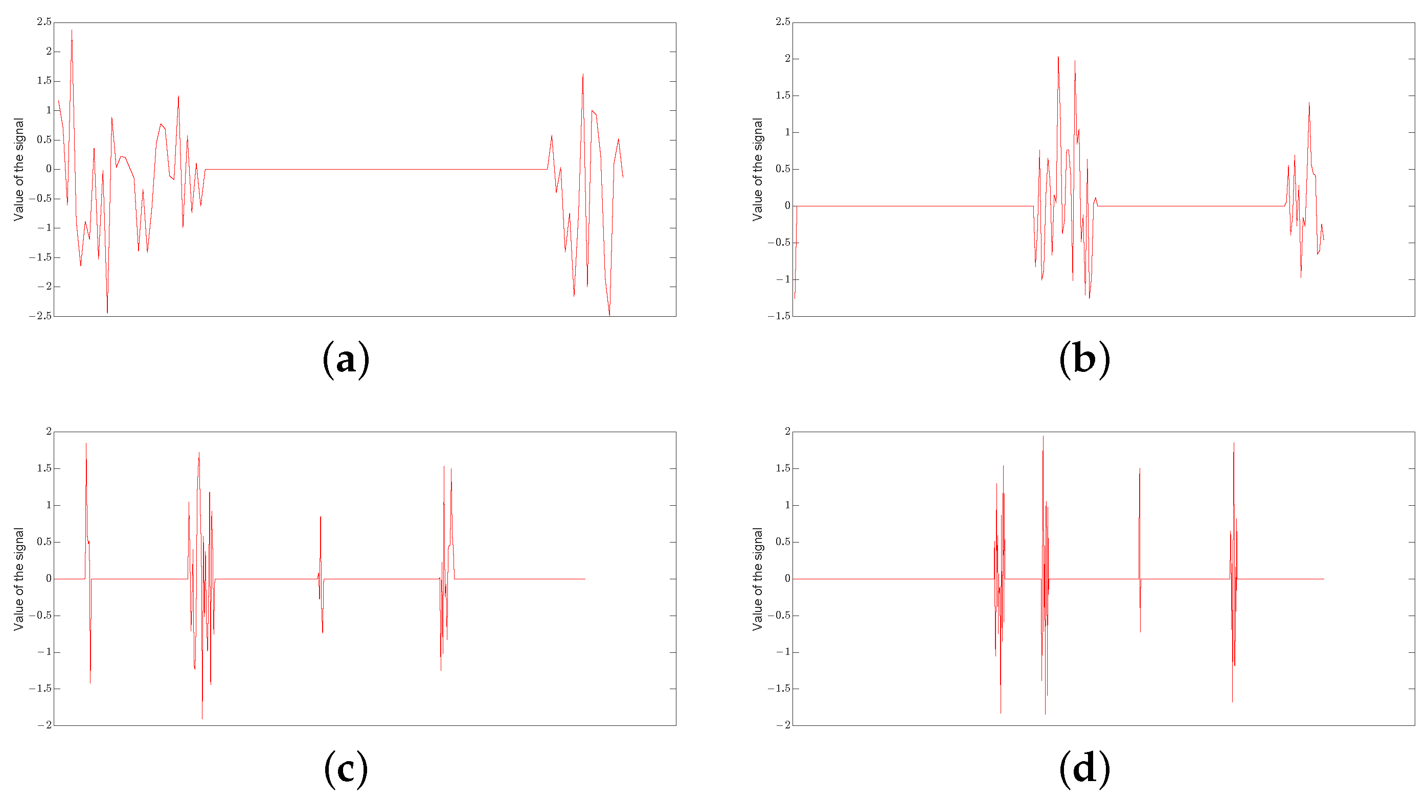
3.2. Effectiveness of the GOMP

Figure 2 shows the performance of the GOMP for an input signal in dimension $N=512$ with group sparsity level $K=50$ and number of measurements $M=200$ under different noises, where the red line represents the original signal and the black squares represent the approximation. Figure 3 shows the performance of BP. The poor performance of BP can be easily observed when the noise occurs.

Figure 2. The recovery of an input signal via GOMP in dimension $N=512$ with group sparsity level $K=50$ and number of measurements $M=200$ under different noises: (a) The recovery of an input signal via GOMP under the noise $e=0$. (b) The recovery of an input signal via GOMP under a Gaussian noise e from $\mathcal{N}(0,{0.1}^2)$.

Figure 3. The recovery of an input signal via BP in dimension $N=512$ with group sparsity level $K=50$ and number of measurements $M=200$ under different noises: (a) The recovery of an input signal via BP under the noise $e=0$. (b) The recovery of an input signal via BP under a Gaussian noise e from $\mathcal{N}(0,{0.1}^2)$.

In general, the above example shows that the GOMP is very effective for signal recovering, i.e., it can recover the group sparse signal exactly. We will analyze the performance of the GOMP further in terms of the mean square error by a comparison with BP in the next subsection.

Figure 4 describes the situation in dimension $d=1024$ under noise $e=0$. It displays the relation between the percentage (of 100 input signals) of the support that can be recovered correctly and the number N of measurements. Furthermore, to some extent, it shows how many measurements are necessary to recover the support of the input group K-sparse signal $x\in {\mathbb{R}}^d$ with high probability. If the percentage equals 100%, it means that support of all the 100 input signals can be found, which implies the support of input signal can be exactly recovered. As expected, Figure 4 shows that when the group sparsity level K increases, it is necessary to increase the number N of measurements to guarantee signal recovery. Furthermore, we can find that the GOMP can recover the correct support of the input signal with high probability.

Figure 4. The percentage of the support of 100 input signals correctly recovered as a function of number N of Gaussian measurements for different group sparsity levels K in dimension $d=1024$.

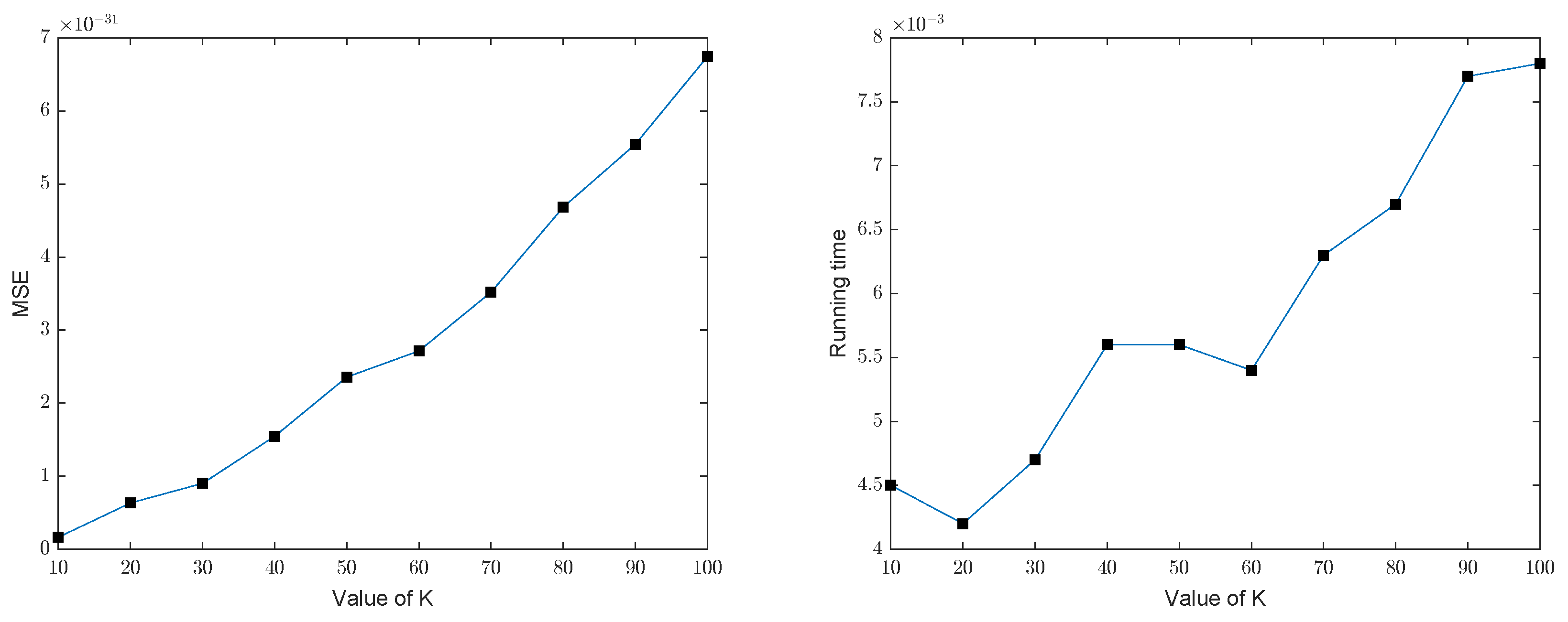
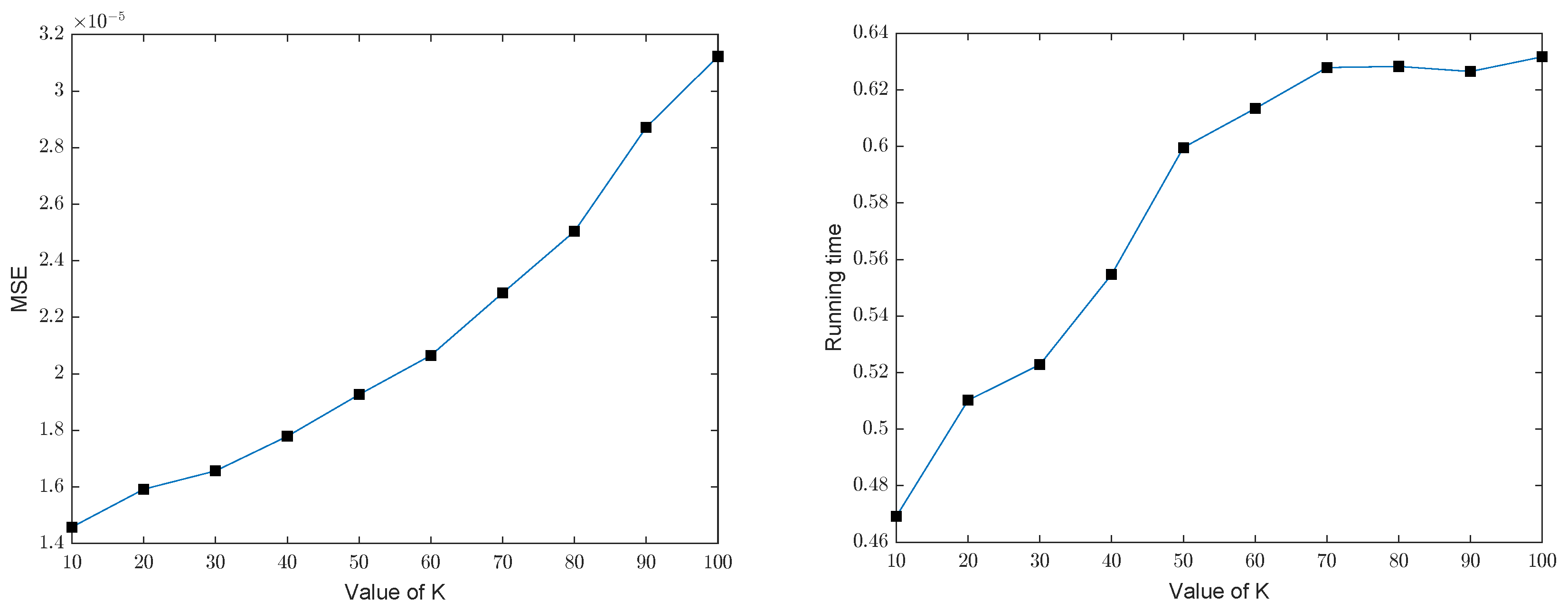
3.3. Comparison with Basis Pursuit

In order to demonstrate the efficiency and robustness of the Group Orthogonal Matching Pursuit (GOMP), we implement the Group Orthogonal Matching Pursuit (GOMP) and the Basis Pursuit (BP) to recover the group sparse signals for comparison.

We implemented the GOMP and BP for recovering the group sparse signals in dimension $N=1024$ with number of measurements $M=500$ under different noises to calculate the average mean square error (MSE) and the average running time by repeating the test 100 times. Figure 5 and Figure 6, respectively, show the MSE and running time of the GOMP, implying that the error and the running time of the GOMP will constantly increase with the increased $K\in \{10,20,\cdots ,100\}$. The figure of the error of the GOMP in terms of MSE is about ${10}^{-31}$ (noiseless) and ${10}^{-7}$ (Gaussian noise), which means that the GOMP can effectively recover the group sparse signal. Meanwhile, the computational complexity of the GOMP is also relatively low according to its running time. Figure 7 and Figure 8 show that the MSE and the running time of the BP have the same trend as the GOMP: the error and the running time increase with the increased sparsity level, without changes to other parameters, while the MSE of BP is higher in figure when compared with the GOMP, which is around ${10}^{-7}$ (noiseless) and ${10}^{-5}$ (Gaussian noise). In order to facilitate comparison, the details of the above results in Figure 5, Figure 6, Figure 7 and Figure 8 also can be found in Table 1 and Table 2.

Figure 5. MSE and running time of the GOMP in dimension $N=1024$ with number of measurements $M=500$ under the noise $e=0$.

Figure 6. MSE and running time of the GOMP in dimension $N=1024$ with number of measurements $M=500$ under a Gaussian noise e from $\mathcal{N}(0,{0.1}^2)$.

Figure 7. MSE and running time of BP in dimension $N=1024$ with number of measurements $M=500$ under the noise $e=0$.

Figure 8. MSE and running time of BP in dimension $N=1024$ with number of measurements $M=500$ under a Gaussian noise e from $\mathcal{N}(0,{0.1}^2)$.

Table 1. The average MSE and running time (repeating 100 times) of the GOMP and BP in 1024 dimension with number of measurements $M=500$ under the noise $e=0$.

Group Sparsity Level	GOMP		BP
	MSE	Running Time	MSE	Running Time
K = 10	$1.6350\times {10}^{-32}$	0.0045s	8.1887 $\times {10}^{-08}$	0.3724 s
K = 20	$6.3295\times {10}^{-32}$	0.0042 s	$8.7195\times {10}^{-8}$	0.5158 s
K = 30	$9.0108\times {10}^{-32}$	0.0047 s	$9.3230\times {10}^{-8}$	0.5358 s
K = 40	$1.5460\times {10}^{-31}$	0.0056 s	$1.0408\times {10}^{-7}$	0.5544 s
K = 50	$2.3565\times {10}^{-31}$	0.0056 s	$1.1414\times {10}^{-7}$	0.4513 s
K = 60	$2.7140\times {10}^{-31}$	0.0054 s	$1.2543\times {10}^{-7}$	0.5099 s
K = 70	$3.5189\times {10}^{-31}$	0.0063 s	$1.4186\times {10}^{-7}$	0.5634 s
K = 80	$4.6822\times {10}^{-31}$	0.0067 s	$1.6007\times {10}^{-7}$	0.5831 s
K = 90	$5.5434\times {10}^{-31}$	0.0077 s	$1.8272\times {10}^{-7}$	0.5946 s
K = 100	$6.7451\times {10}^{-31}$	0.0078 s	$2.0194\times {10}^{-7}$	0.6087 s

Table 2. The average MSE and running time (repeating 100 times) of the GOMP and BP in 1024 dimension with number of measurements $M=500$ under a Gaussian noise e from $\mathcal{N}(0,{0.1}^2)$.

Group Sparsity Level	GOMP		BP
	MSE	Running Time	MSE	Running Time
K = 10	$2.1440\times {10}^{-7}$	0.0043 s	1.4580 $\times {10}^{-5}$	0.4691 s
K = 20	$4.1167\times {10}^{-7}$	0.0043 s	$1.5919\times {10}^{-5}$	0.5102 s
K = 30	$6.1894\times {10}^{-7}$	0.0050 s	$1.6566\times {10}^{-5}$	0.5228 s
K = 40	$8.6262\times {10}^{-7}$	0.0058 s	$1.7790\times {10}^{-5}$	0.5547 s
K = 50	$1.1870\times {10}^{-6}$	0.0058 s	$1.9266\times {10}^{-5}$	0.5996 s
K = 60	$1.3162\times {10}^{-6}$	0.0057 s	$2.0652\times {10}^{-5}$	0.6134 s
K = 70	$1.6356\times {10}^{-6}$	0.0067 s	$2.2859\times {10}^{-5}$	0.6279 s
K = 80	$1.9119\times {10}^{-6}$	0.0069 s	$2.5038\times {10}^{-5}$	0.6283 s
K = 90	$2.1399\times {10}^{-6}$	0.0076 s	$2.8718\times {10}^{-5}$	0.6265 s
K = 100	$2.5990\times {10}^{-6}$	0.0081 s	$3.1227\times {10}^{-5}$	0.6317 s

According to the mean square error, obviously our algorithm outperforms the BP by a lot on both noiseless and noisy data. This trend is expected because the solution of the GOMP is updated by solving least squares problems. What is more, the BP normally cannot exactly recover the real signal since the produced solution may not be 0 on the indices which are not in the support, according to the observation during the experiments (can also be found in Figure 3b. For the GOMP, the solution’s support has been restricted in the group sparse set based on the selected indices of the group structure ${\left\{G\right\}}_{i=1}^g$ at each iteration. That also leads to the better performance of the GOMP compared with BP. Although the performance of the GOMP can be affected by the group sparsity level and noise, our method still has pretty low mean square errors and performs better than BP, showing the robustness and effectiveness of our proposed algorithm. We can also observe that the GOMP runs much quicker than the BP, demonstrating the scalability and efficiency of our algorithm.

Further more, when it comes to large-scale group sparse signal recovery, the execution of BP occupies more memory and takes far more time to obtain the solution compared with our method (details can be found in Table 3 and Table 4 for different noise scenarios). This is because the scale of least square problems that the GOMP needs to solve to obtain the solution are bounded by the sparsity level K, as seen in the GOMP defined in Section 1. At the same time, the GOMP still outperforms BP a lot in terms of MSE. In addition, we can also find that the running speed of BP will be slightly slower when the noise occurs, while for the GOMP it will not be affected.

Table 3. The average MSE and running time (repeating 100 times) of the GOMP and BP with number of measurements $M=500$ and group sparsity level $K=50$ under the noise $e=0$.

Dimension	GOMP		BP
	MSE	Running Time	MSE	Running Time
N = 1024	$2.3846\times {10}^{-31}$	0.0057 s	$1.1414\times {10}^{-7}$	0.4513 s
N = 2048	$1.1178\times {10}^{-31}$	0.0114 s	$4.4095\times {10}^{-8}$	1.6611 s
N = 3072	$8.5425\times {10}^{-32}$	0.0195 s	$2.7722\times {10}^{-8}$	5.8170 s
N = 4096	$5.9586\times {10}^{-32}$	0.0413 s	$1.9752\times {10}^{-8}$	11.3636 s

Table 4. The average MSE and running time (repeating 100 times) of the GOMP and BP with number of measurements $M=500$ and group sparsity level $K=50$ under a Gaussian noise e from $\mathcal{N}(0,{0.1}^2)$.

Dimension	GOMP		BP
	MSE	Running Time	MSE	Running Time
N = 1024	$1.1143\times {10}^{-6}$	0.0066 s	$1.9539\times {10}^{-5}$	0.4521 s
N = 2048	$5.7826\times {10}^{-7}$	0.0115 s	$7.8597\times {10}^{-6}$	2.6113 s
N = 3072	$3.9382\times {10}^{-7}$	0.0200 s	$5.3449\times {10}^{-6}$	6.3476 s
N = 4096	$3.0434\times {10}^{-7}$	0.0406 s	$4.4554\times {10}^{-6}$	12.1959 s

4. Conclusions

We propose the Group Orthogonal Matching Pursuit (GOMP) to recover group sparse signals. We analyze the error of the GOMP algorithm in the process of recovering group sparse signals from noisy measurements. We show the instance optimality and robustness of the GOMP under the group restricted isometry property (GRIP) of the decoder matrix. Compared with the P-norm minimization approach, the GOMP has two advantages. One is its easier implementation, that is, it runs quickly and has lower computational complexity. The other is that we do not need the concept of $\gamma$-decomposability. Furthermore, our simulation results show that the GOMP is very efficient for group sparse signal recovery and significantly outperforms Basis Pursuit in both scalability and solution quality.

On the other hand, there are several algorithms that we will study in the future, such as Sparsity Adaptive Matching Pursuit (SAMP) [34], Constrained Backtracking Matching Pursuit (CBMP) [35] and Group-based Sparse Representation-Joint Regularization (GSR-JR) [36], which could be potentially competitive with the GOMP.

References

- Foucart, S.; Rauhut, H. A Mathematical Introduction to Compressive Sensing; Springer: Berlin/Heidelberg, Germany, 2013. [Google Scholar]
- Cai, T.; Zhang, A. Sparse representation of a polytope and recovery of sparse signals and low-rank matrices. IEEE Trans. Inf. Theory 2014, 60, 122–132. [Google Scholar] [CrossRef]
- Günther, M.; Böhringer, S.; Wieczorek, D.; Würtz, R.P. Reconstruction of images from Gabor graphs with applications in facial image processing. Int. J. Wavelets Multiresolut. Inf. Process. 2015, 13, 1550019. [Google Scholar] [CrossRef]
- Ye, P.X.; Wei, X.J. Efficiency of weak greedy algorithms for m-term approximations. Sci. China. Math. 2016, 59, 697–714. [Google Scholar] [CrossRef]
- Yang, B.; Yang, C.; Huang, G. Efficient image fusion with approximate sparse representation. Int. J. Wavelets Multiresolut. Inf. Process. 2016, 14, 1650024. [Google Scholar] [CrossRef]
- Candès, E.; Kalton, N.J. The restricted isometry property and its implications for compressed sensing. C. R. Acad. Sci. Sér. I 2008, 346, 589–592. [Google Scholar] [CrossRef]
- Candès, E.J.; Tao, T. Decoding by linear programming. IEEE Trans. Inf. Theory 2005, 51, 4203–4215. [Google Scholar] [CrossRef]
- Yuan, M.; Lin, Y. Model selection and estimation in regression with grouped variables. J. R. Stat. Ser. B 2006, 68, 49–67. [Google Scholar] [CrossRef]
- Ou, W.; Hämäläinen, M.S.; Golland, P. A distributed spatio-temporal EEG/MEG inverse solver. NeuroImage 2009, 44, 932–946. [Google Scholar] [CrossRef]
- Antoniadis, A.; Fan, J. Regularization of wavelet approximations. J. Amer. Stat. Assoc. 2001, 96, 939–967. [Google Scholar] [CrossRef]
- He, Z.; Yu, W. Stable feature selection for biomarker discovery. Comput. Biol. Chem. 2010, 34, 215–225. [Google Scholar] [CrossRef]
- Mishali, M.; Eldar, Y.C. Blind multiband signal reconstruction: Compressed sensing for analog signals. IEEE Trans. Signal Process. 2009, 57, 993–1009. [Google Scholar] [CrossRef]
- Ahsen, M.E.; Vidyasagar, M. Error bounds for compressed sensing algorithms with group sparsity: A unified approach. Appl. Comput. Harmon. Anal. 2017, 42, 212–232. [Google Scholar] [CrossRef]
- Ranjan, S.; Vidyasagar, M. Tight performance bounds for compressed sensing with conventional and group sparsity. IEEE Trans. Signal Process 2019, 67, 2854–2867. [Google Scholar] [CrossRef]
- Tropp, J.A. Greedy is good: Algorithmic results for sparse approximation. IEEE Trans. Inform. Theory 2004, 50, 2231–2242. [Google Scholar] [CrossRef]
- Lin, J.H.; Li, S. Nonuniform support recovery from noisy measurements by orthogonal matching pursuit. J. Approx. Theory 2013, 165, 20–40. [Google Scholar] [CrossRef]
- Mo, Q.; Shen, Y. A remark on the restricted isometry property in orthogonal matching pursuit. IEEE Trans. Inf. Theory 2012, 58, 3654–3656. [Google Scholar] [CrossRef]
- Dan, W. Analysis of orthogonal multi-matching pursuit under restricted isometry property. Sci. China Math. 2014, 57, 2179–2188. [Google Scholar] [CrossRef]
- Xu, Z.Q. The performance of orthogonal multi-matching pursuit under RIP. J. Comp. Math. 2015, 33, 495–516. [Google Scholar] [CrossRef]
- Shao, C.F.; Ye, P.X. Almost optimality of orthogonal super greedy algorithms for incoherent dictionaries. Int. J. Wavelets Multiresolut. Inf. Process. 2017, 15, 1750029. [Google Scholar] [CrossRef]
- Wei, X.J.; Ye, P.X. Efficiency of orthogonal super greedy algorithm under the restricted isometry property. J. Inequal. Appl. 2019, 124, 1–21. [Google Scholar] [CrossRef]
- Zhang, T. Sparse recovery with orthogonal matching pursuit under RIP. IEEE Trans. Inf. Theory 2011, 57, 6215–6221. [Google Scholar] [CrossRef]
- Xu, Z.Q. A remark about orthogonal matching pursuit algorithm. Adv. Adapt. Data Anal. 2012, 04, 1250026. [Google Scholar] [CrossRef]
- Cohen, A.; Dahmen, W.; DeVore, R. Orthogonal matching pursuit under the restricted isometry property. Constr. Approx. 2017, 45, 113–127. [Google Scholar] [CrossRef]
- Eldar, Y.C.; Mishali, M. Robust recovery of signals from a structured union of subspaces. IEEE Trans. Inf. Theory 2009, 55, 5302–5316. [Google Scholar] [CrossRef]
- Wright, J.; Yang, A.Y.; Ganesh, A.; Sastry, S.S.; Ma, Y. Robust face recognition via sparse representation. IEEE Trans. Pattern Anal. Mach. Intell. 2009, 31, 210–227. [Google Scholar] [CrossRef]
- Van Den Berg, E.; Friedlander, M.P. Theoretical and empirical results for recovery from multiple measurements. IEEE Trans. Inf. Theory 2010, 56, 2516–2527. [Google Scholar] [CrossRef]
- Eldar, Y.C.; Kuppinger, P.; Bölcskei, H. Block-sparse signals: Uncertainty relations and efficient recovery. IEEE Trans. Signal Process. 2010, 58, 3042–3054. [Google Scholar] [CrossRef]
- Lai, M.J.; Liu, Y. The null space property for sparse recovery from multiple measurement vectors. Appl. Comput. Harmon. Anal. 2011, 30, 402–406. [Google Scholar] [CrossRef]
- Zhang, J.; Wang, J.; Wang, W. A perturbation analysis of block-sparse compressed sensing via mixed l2/l1 minimization. Int. J. Wavelets, Multiresolut. Inf. Process. 2016, 14, 1650026. [Google Scholar] [CrossRef]
- Chen, W.G.; Ge, H.M. A sharp recovery condition for block sparse signals by block orthogonal multi-matching pursuit. Sci. China Math. 2017, 60, 1325–1340. [Google Scholar] [CrossRef]
- Wen, J.M.; Zhou, Z.C.; Liu, Z.L.; Lai, M.J.; Tang, X.H. Sharp sufficient conditions for stable recovery of block sparse signals by block orthogonal matching pursuit. Appl. Comput. Harmon. Anal. 2019, 47, 948–974. [Google Scholar] [CrossRef]
- Candès, E.; Romberg, J. l1-Magic: Recovery of Sparse Signals via Convex Programming. Available online: https://candes.su.domains/software/l1magic/#code (accessed on 15 February 2023).
- Do, T.T.; Gan, L.; Nguyen, N.; Tran, T.D. Sparsity adaptive matching pursuit algorithm for practical compressed sensing. In Proceedings of the 2008 42nd Asilomar Conference on Signals, Systems and Computers, Pacific Grove, CA, USA, 26–29 October 2008; pp. 581–587. [Google Scholar]
- Bi, X.; Leng, L.; Kim, C.; Liu, X.; Du, Y.; Liu, F. Constrained Backtracking Matching Pursuit Algorithm for Image Reconstruction in Compressed Sensing. Appl. Sci. 2021, 11, 1435. [Google Scholar] [CrossRef]
- Wang, R.; Qin, Y.; Wang, Z.; Zheng, H. Group-Based Sparse Representation for Compressed Sensing Image Reconstruction with Joint Regularization. Electronics 2022, 11, 182. [Google Scholar] [CrossRef]
Disclaimer/Publisher’s Note: The statements, opinions and data contained in all publications are solely those of the individual author(s) and contributor(s) and not of MDPI and/or the editor(s). MDPI and/or the editor(s) disclaim responsibility for any injury to people or property resulting from any ideas, methods, instructions or products referred to in the content. |
© 2023 by the authors. Licensee MDPI, Basel, Switzerland. This article is an open access article distributed under the terms and conditions of the Creative Commons Attribution (CC BY) license (https://creativecommons.org/licenses/by/4.0/).