1. Introduction
Finite mixture distributions have a rich legacy in statistics. Newcomb [
1] originated the idea of the finite mixture models for modelling outliers. The finite mixture distribution is a potent and adaptable probabilistic modelling framework for both univariate and multivariate data. The mixture model is broadly recognized in the field of statistical data modelling [
2]. Pearson [
3] used a mixture of two univariate Gaussian models to evaluate model parameters using the method of moments to examine a dataset comprising forehead-to-body length ratios for 1000 crabs. When a mixture model replaces a poor single model, the fitting effect of the load data (such as the wheel loader) improves [
4]. Since then, several scholars have investigated finite mixture models in diverse circumstances. The load range probability density function can be characterized as a mixture of Weibull models [
5,
6]. Ni Yiqing [
7] modelled the stress range using three types of finite mixture models (normal, lognormal, and Weibull). Radhakrishna et al. [
8] investigated the moment and maximum likelihood estimators of the uncertain parameters of a mixture of the generalized gamma model. To forecast the collapse of a mechanical framework with multiple risks modes, Zhang et al. [
9] introduced a mixture Weibull proportional hazard model. In contrast, [
10] described the exponential mixture model and the increasing failure rate of Gamma models. Damsesy et al. [
11] estimated the reliability and malfunction rate of an electronic system using a mixture of two Lindley models. [
12] on the other hand presented and explored a finite mixture of Lindley models and its stress–strength reliability. Several scholars who deal with mixture modelling in various practical concerns are listed below: Mohammadi et al. [
13,
14], Ateya [
15], and Sindhu et al. [
16]. Other research findings are [
17,
18,
19,
20,
21,
22,
23].
Since the family of exponential models is significant in several application scenarios, we will investigate a mixture of two log-Bilal (LB) distributions that belong to this family and are utilized in several implementations. In this respect, the Lindley model is useful for characterizing diverse sets of lifespan data and reliability. Even though the beta model is commonly utilized to model data sets with bounded intervals, it fails to model extremely left-skewed and leptokurtic data sets. The LB distribution eradicates the shortcomings of existing models for modelling extremely skewed data sets. This model is required because it offers more versatility than established models for the shapes of the hazard function (HF), and this distribution completes well in modelling lifespan data and is a better option than other models [
24]. The different estimation methods for analysis of unknown parameters are used to investigate the efficiency of different methodologies in distribution studies. Recently Sindhu et al. [
25] tried to use different estimation methods to estimate the mixture distribution. The highlights of their study have proposed that the mixture model is a potential candidate for modelling COVID-19 and other associated data sets.
From the cited literature, it has been revealed that many researchers have been focused on mixture distributions over an infinite domain, but not much attention has been given to model data sets on bounded intervals with mixture models. So, in this research work, we determined to present this novel mixture model and explain its characteristics and implementations from a different perspective. Hence, we develop and investigate the MLBD in detail. We also explain the assessment of the unspecified parameters of the mixture model, employing appropriate techniques such as the maximum likelihood least-squares estimation (LSE) and weighted least-squares estimation (WLSE). Lastly, we conduct some simulation experiments and apply a real-world dataset to the MLBDs. As a necessary consequence, we use goodness-of-fit strategies with some plots of a histogram and likelihood function for the dataset to endorse and highlight data fitting via some packages in the R programming language. The novelty of the current work is described in the following lines.
To construct a new two-component mixture of a LB distribution which has simple- and closed-form equations for its statistical characteristic.
We illustrate some graphs of the unimodal and bimodal cases of the mixture model density and hazard rate functions.
The properties of the MLBDs are obtained in explicit forms without any special mathematical functions.
The main focus of this work is to analyze the different method of estimation and to carry out a comparative study for estimation for the mixture model. This comparison will be expressed with the help of statistical graphs.
The feasibility and effectiveness of this model is proven through the simulation study and a real dataset.
2. Model Analysis and General Properties of the MLBDs
The mixture distribution function of the MLBDs of component densities with weighting proportions
has the following PDF (probability density function).
which complies with the following limitations:
where
signifies a vector of component unexplained
parameters. Constant
ξ symbolizes
for a weighting proportion, and
symbolizes a component PDF of log-Bilal distribution (LBD). The LBD is expressed by the random variable (
r.v) Y that has the presenting PDF.
where
ξi denotes the scale parameter. The CDF (Cumulative Distribution Function) of the MLBD is
Hazard rate functions (HRF) are essential components of lifetime distributions. Most applications use this information to show how failure risk shifts over time. It may be helpful to have prior knowledge about the shape of the hazard when choosing a model. The HRF of MLBDs is:
2.1. Mean and Variance:
The Mean of MLBDs in (1) is simply given as Whereas the variance is described as
2.2. kth Moments
The kth Moments of theMLBDsis presented as 2.3. mth Order Negative Moments
The mth Order Negative Moment can be simply obtained by substituting k with “m” in (8), as shown below 2.4. Factorial Moments: The Factorial Moments Can Be Measured Using [26] Result as Given
here
denotes the non-null real numbers. The
can be simply determined by substituting
k with “
m” in (8), as
2.5. Mode and Median
It can be demonstrated that equations for acquiring the mode and median of the MLBDs are 2.6. Incomplete Moments
The kthIncomplete Moment of Y is The incomplete moments of random variables are useful techniques for measuring inequalities, such as the Gini coefficient (see, [
27] for details).
Figure 1a–e shows the PDF configurations of the MLBDs for both unimodal and bimodal contexts.
Figure 1a–d depicts the PDF of the MLBDs unimodal case at the specified values of parameters and
Figure 1e captures the structure of the MLBDs bimodal case with the
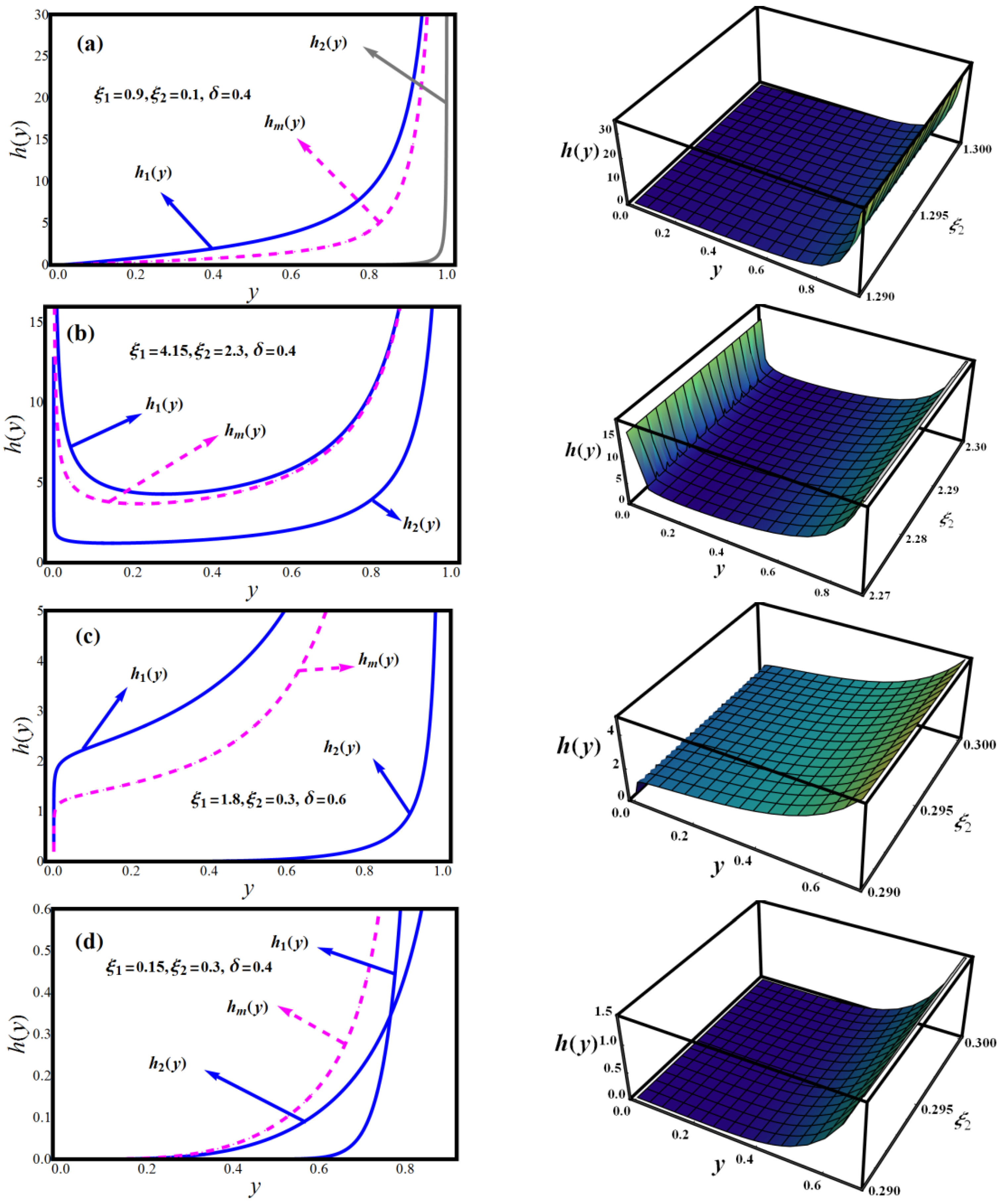
The visual behavior of the hrf
h(
y) of the MLBDs is shown in
Figure 2a–d. The hazard rate of the MLBDs distribution comes in a variety of shapes, including, increasing, and bathtub curves, all of which are appealing features for any lifespan model.
Figure 3 and
Figure 4 display the mean plots of the MLBDs distribution, showing decreasing behavior. The variance plots of the MLBDs are shown in
Figure 5, where they exhibit increasing and upside-down behavior.
3. Estimation
We go over the method for estimating the parameters of the MLBDs using four estimation methods. These certain approaches are MLE (maximum likelihood estimation), LSE (least-squares estimation), and WLSE (weighted least-squares estimation). The rest of this section contains more information on these estimation techniques.
3.1. Maximum Likelihood
Let
be a random sample from the MLBDs and corresponding given values
from the MLBD with parameters
The log-likelihood function of MLBDs is
By differentiating (15) with respect to
gives
The MLEs of parameters, is the solution of (16)–(18) for zero. There is no clear and specific analytic expression for (11). As a matter of fact, it can be addressed iteratively, or the direct maximization of (15) can be considered as an alternative. Similarly, the immediate maximization of (15) is selected by utilizing the optimum tool of the R programming language.
3.2. Least Squares
Let
be the arranged values of
having MLBDs. The LSE of
is assessed by minimizing.
where
is in (3). Then,
3.3. Weighted Least Squares
The minimization of (21) gives the WLS estimators of parameters
.
4. Simulation Study and Comparisons
We examine the effectiveness of the MLE, LSE, and WLSE mechanisms in assessing the parameters of the MLBDs. As a result, we conduct Monte Carlo (MC) simulation investigations on the unimodal and bimodal cases of a MLBDs.
Four simulation experiments are performed in order to examine the effectiveness of MLEs, LSEs, and WLSEs of the MLBDs. The simulation algorithm is explained in the steps below:
Utilizing various weighting factor and model parameters for the unimodal and bimodal scenarios, develop random samples of sizes from the mixture model MLBDs. The random samples for the simulation are obtained in the following step.
Start generating one variable u from the distribution using (runif) in R.
If then we create a random variable from the first component (LBD with ). If , we develop a random variable from the second component (LBD with ).
Continue with (2) till we have the requisite sample of size n.
Using 1000 replications, keep repeating steps 1 to 4 again. Compute the MLEs, LSEs, and WLSEs for the 1000 samples; if for to acquire numerical outcomes for the simulation experiment, the statistical software R is employed. The following quantities are used to interpret the simulation results.
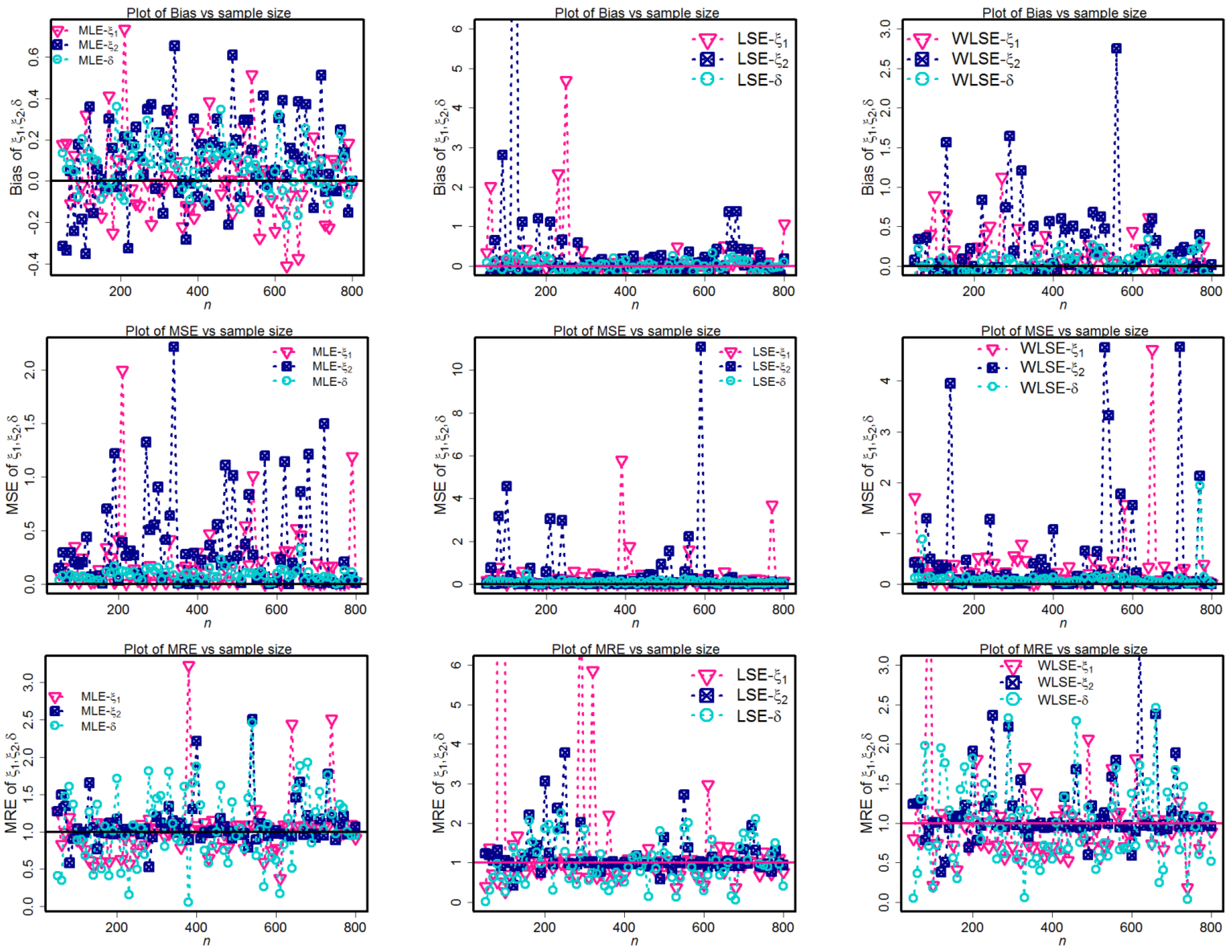
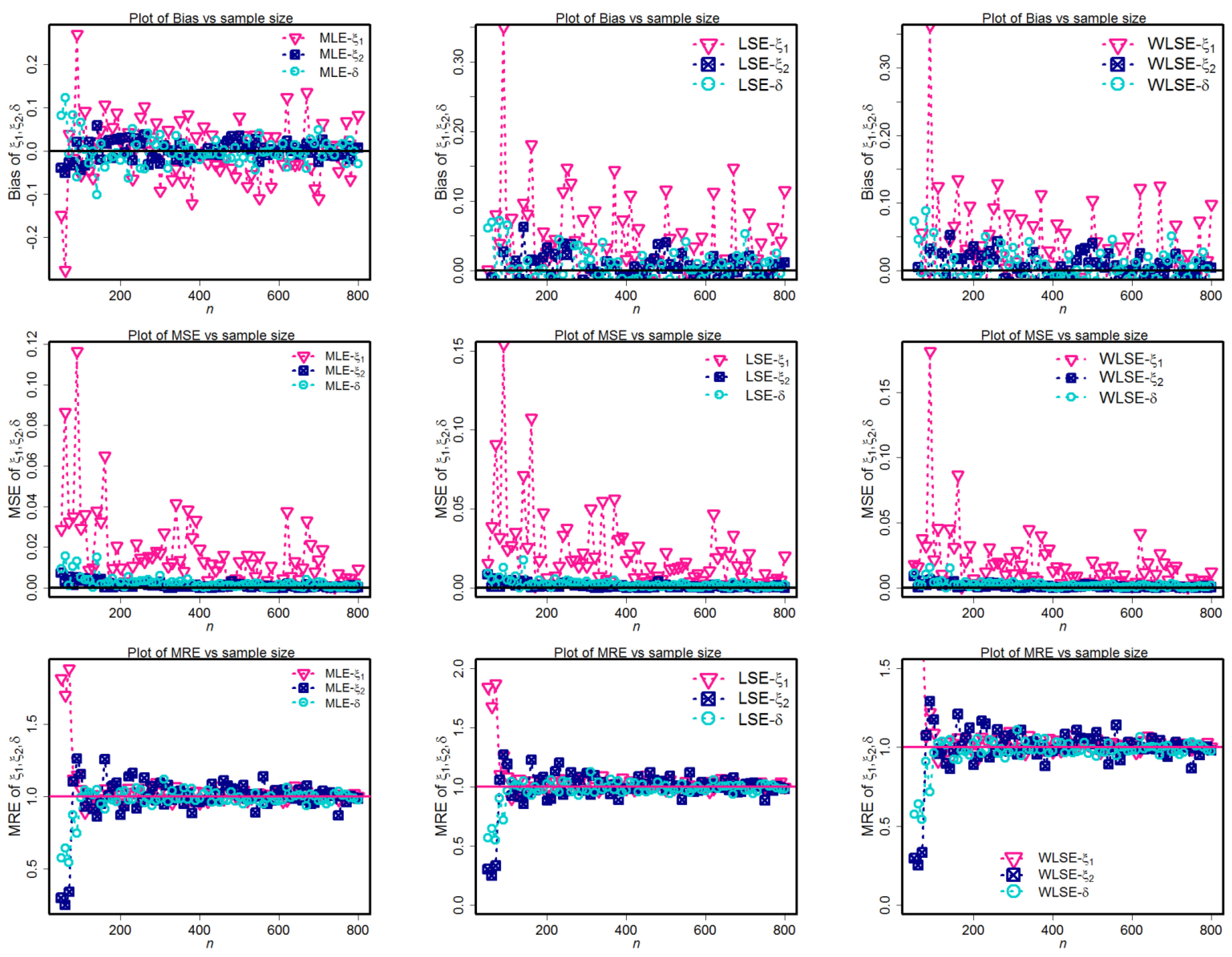
These quantitative metrics, such as the mean squared errors (MSEs) and mean relative errors (MREs), are utilized to evaluate the various methods of determining the ideal model under pre-ascertained possibilities (see, Zeng et al., [
28]). If the forecasting models produce an asymptotically unbiased estimate, we can expect MSEs and biases to reach zero. MREs, in contrast, will be very close to one.
Figure 6,
Figure 7,
Figure 8 and
Figure 9 depict the simulation findings. These graphs show that the MLE technique approaches the optimum condition of biases, MSEs, and MREs quicker than other evaluation techniques for component parameters and weighted factors. As a direct consequence, the MLE method is superior to other methods for estimating the MLBD parameters.
5. Empirical Studies
The data set, called the trade share data set, takes into account the readings of the variable trade share in the well-known “Determinants of Economic Growth Data.” Up to 61 countries’ growth rates, as well as characteristics that may be associated with growth, are studied. As an online supplement to [
29], the data are publicly available. In [
30], scholars investigate this data set as well. The data on trade share is right-skewed or almost symmetrical and the value of excess kurtosis shows distribution is thin-tailed or close to platykurtic with a moderate standard deviation, as seen in
Table 1.
We investigate this data set using a fitting strategy as our primary statistical study. The MLBDs distribution has been validated with the mixture of two unit-Lindley models [
31] and a mixture of two log-X Lindley models [
25] on a real-world data set to demonstrate its capabilities. As comparison criteria, the fitted distributions are compared by utilizing goodness-of-fit indicators such as AIC (Akaike information), CAIC (consistent Akaike information), the log likelihood (
l (.)) value where
l (.) represents the maximized score of the log-likelihood function, and BIC (Bayesian information).
Table 2 displays the outcomes of the estimations, model adequacy measures, and data fitting statistics. It is worth noting that the MLBDs model produces the greatest log-likelihood value [
32,
33]. The optimal model for the data sets is one with the lowest values of these model adequacy metrics but the highest value of the log-likelihood function.
Figure 10 combines boxplot and histograms to depict the quantile characteristics and layout of the data set. In addition, a strip chart for the data set is also shown in
Figure 10. The strip chart produces one-dimensional scatter plots (also referred as dot plots) of the input data. When sample sizes are small, these plots are useful replacements for boxplots. The projections of the modelled CDF, SF, and P–P plots for the data set are also discussed in
Figure 11 and
Figure 12.
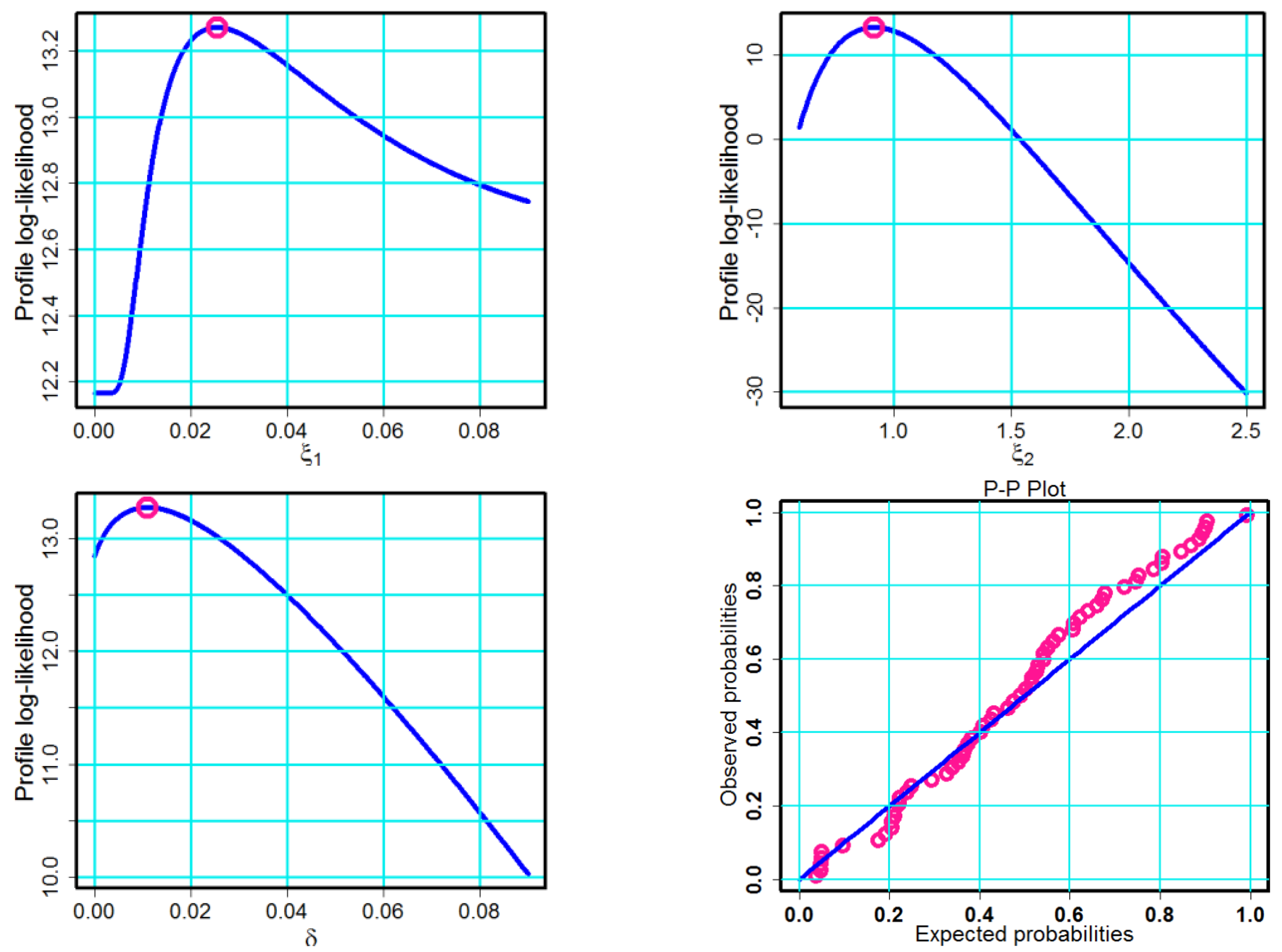
For this data, the estimated variance–covariance matrix
of the MLBDs is given using
The estimated parameters maximize the log-likelihood function, as seen in
Figure 11. With Mathematica 12, we estimate the roots with the help of the NMaximize function that invariably determines the global maximum, not the local maximum. We also confirmed these findings by plotting the log-likelihood function; as shown, the deep-pink dot indicates that the estimates are at their highest points across the curve.
Result Reveals from the Analysis of the Dataset
As a result, we can infer that the MLBDs model conforms better than the other contending models.
Table 2 reveals that the MLBDs distribution contains the lowest scores with the highest value of the log-likelihood function when compared to certain other distributions on all information metrics.
Furthermore, when the distribution is the MLBDs, the value of l (.) is the highest. As a result, we can conclude that MLBDs better fits the trade share dataset.
The PP plot in
Figure 11 indicates that the proposed model is a good match and model for dataset.
The estimated CDF and SF of the model plots are shown in
Figure 11 indicate that the proposed model is a good fit for data set.
The log-likelihood function has a global maximum root for the model parameters, as demonstrated in
Figure 11.
6. Conclusions
We studied a mixture of two one-parameter log-Bilals (MLBDs) in this investigation utilizing three estimate methods: the MLE, LSE, and WLSE. Additionally, some additional statistical characteristics of the MLBDs model were noticed. A total of 1000 replications were used in a simulation investigation to evaluate and compare the effectiveness of the estimation methodologies. As a result, we revealed that when assessing the model’s unknown parameters, the MLE technique executed better than the alternatives in terms of accuracy and consistency. This innovative model has been applied in trade share data. The histogram, CDF, SF, and PP curves/plots are also useful for determining the best fit to confine datasets. We illustrated that the MLBDs model is appropriate and successful for data modelling, and that it performs better with the mixture of two unit-Lindley and two log-X Lindley using a real dataset. We may utilize the proposed model to model diverse real data sets in a variety of areas in the future, such as medical diagnosis, systems engineering, survival research, and so forth.
Author Contributions
Conceptualization, S.A.L., T.N.S.; data curation, T.N.S., M.K.H.H.; formal analysis, S.A.L., T.N.S., S.A.A.; investigation, T.A.A., T.N.S., M.K.H.H.; methodology, T.N.S., M.K.H.H., S.A.; software, T.N.S., and T.A.A.; validation, S.A.L., T.N.S., M.K.H.H., S.A.A.; writing—original draft, T.N.S., M.K.H.H.; writing—review and editing, T.N.S., S.A. and T.A.A. All authors have read and agreed to the published version of the manuscript.
Funding
This research received no external funding.
Institutional Review Board Statement
Not applicable.
Informed Consent Statement
Not applicable.
Data Availability Statement
The datasets generated and analyzed during the current research are available from the corresponding author on reasonable request.
Conflicts of Interest
The authors declare that they have no conflicts of interest.
References
- Newcomb, S. A generalized theory of the combination of observations so as to obtain the best result. Am. J. Math. 1886, 8, 343–366. [Google Scholar] [CrossRef]
- Pearson, K. Contributions to the mathematical theory of evolution. Philos. Trans. R. Soc. London A 1894, 185, 71–110. [Google Scholar]
- Figueiredo, M.A.T.; Jain, A.K. Unsupervised learning of finite mixture models. IEEE Trans. Pattern Anal. Mach. Intell. 2002, 24, 381–396. [Google Scholar] [CrossRef]
- Nagode, M.; Klemenc, J.; Fajdiga, M. Parametric modelling and scatter prediction of rainflow matrices. Int. J. Fatigue 2001, 23, 525–532. [Google Scholar] [CrossRef]
- Nagode, M.; Fajdiga, M. On a new method for prediction of the scatter of loading spectra. Int. J. Fatigue 1998, 20, 271–277. [Google Scholar] [CrossRef]
- Tovo, R. On the fatigue reliability evaluation of structural components under service loading. Int. J. Fatigue 2001, 23, 587–598. [Google Scholar] [CrossRef]
- Ni, Y.Q.; Ye, X.W.; Ko, J.M. Modeling of stress spectrum using long-term monitoring data and finite mixture distributions. J. Eng. Mech. 2012, 138, 175–183. [Google Scholar] [CrossRef]
- Radhakrishna, C.; Dattatreya Rao, A.V.; Anjaneyulu, G.V.S.R. Estimation of parameters in a two-component mixture generalized gamma distribution. Commun. Stat. Theory Methods 1992, 21, 1799–1805. [Google Scholar] [CrossRef]
- Zhang, Q.; Hua, C.; Xu, G. A mixture Weibull proportional hazard model for mechanical system failure prediction utilizing lifetime and monitoring data. Mech. Syst. Signal Process. 2014, 43, 103–112. [Google Scholar] [CrossRef]
- Block, H.W.; Langberg, N.A.; Savits, T.H. A mixture of exponential and IFR gamma distributions having an upside-down bathtub-shaped failure rate. Probab. Eng. Inf. Sci. 2012, 26, 573–580. [Google Scholar] [CrossRef]
- Damsesy, M.A.E.; El Genidy, M.M.; El Gazar, A.M. Reliability and failure rate of the electronic system by using mixture Lindley distribution. J. Appl. Sci. 2015, 15, 524–530. [Google Scholar] [CrossRef][Green Version]
- Khan, A.H.; Jan, T.R. Estimation of stress-strength reliability model using finite mixture of two parameter Lindley distributions. J. Stat. Appl. Probab. 2015, 4, 147–159. [Google Scholar]
- Mohammadi, A.; Salehi-Rad, M.R.; Wit, E.C. Using mixture of Gamma distributions for Bayesian analysis in an M/G/1 queue with optional second service. Comput. Stat. 2013, 28, 683–700. [Google Scholar] [CrossRef]
- Mohamed, M.M.; Saleh, E.; Helmy, S.M. Bayesian prediction under a finite mixture of generalized exponential lifetime model. Pak. J. Stat. Oper. Res. 2014, 10, 417–433. [Google Scholar] [CrossRef]
- Ateya, S.F. Maximum likelihood estimation under a finite mixture of generalized exponential distributions based on censored data. Stat. Pap. 2014, 55, 311–325. [Google Scholar] [CrossRef]
- Sindhu, T.N.; Aslam, M. Preference of prior for Bayesian analysis of the mixed Burr type X distribution under type I censored samples. Pak. J. Stat. Oper. Res. 2014, 10, 17–39. [Google Scholar] [CrossRef]
- Zhang, H.; Huang, Y. Finite mixture models and their applications: A review. Austin Biom. Biostat. 2015, 2, 1–6. [Google Scholar]
- Sindhu, T.N.; Riaz, M.; Aslam, M.; Ahmed, Z. Bayes estimation of Gumbel mixture models with industrial applications. Trans. Inst. Meas. Control 2016, 38, 201–214. [Google Scholar] [CrossRef]
- Sindhu, T.N.; Aslam, M.; Hussain, Z. A simulation study of parameters for the censored shifted Gompertz mixture distribution: A Bayesian approach. J. Stat. Manag. Syst. 2016, 19, 423–450. [Google Scholar] [CrossRef]
- Sindhu, T.N.; Feroze, N.; Aslam, M.; Shafiq, A. Bayesian inference of mixture of two Rayleigh distributions: A new look. Punjab Univ. J. Math. 2020, 48, 49–64. [Google Scholar]
- Sindhu, T.N.; Khan, H.M.; Hussain, Z.; Al-Zahrani, B. Bayesian Inference from the Mixture of Half-Normal Distributions under Censoring. J. Natl. Sci. Found. Sri Lanka 2018, 46, 587–600. [Google Scholar] [CrossRef]
- Sindhu, T.N.; Hussain, Z.; Aslam, M. Parameter and reliability estimation of inverted Maxwell mixture model. J. Stat. Manag. Syst. 2019, 22, 459–493. [Google Scholar] [CrossRef]
- Ali, S. Mixture of the inverse Rayleigh distribution: Properties and estimation in a Bayesian framework. Appl. Math. Model. 2015, 39, 515–530. [Google Scholar] [CrossRef]
- Altun, E.; El-Morshedy, M.; Eliwa, M.S. A new regression model for bounded response variable: An alternative to the beta and unit-Lindley regression models. PLoS ONE 2021, 16, e0245627. [Google Scholar] [CrossRef]
- Sindhu, T.N.; Hussain, Z.; Alotaibi, N.; Muhammad, T. Estimation method of mixture distribution and modeling of COVID-19 pandemic. AIMS Math. 2022, 7, 9926–9956. [Google Scholar] [CrossRef]
- Khan, M.N. The modified beta Weibull distribution. Hacet. J. Math. Stat. 2015, 44, 1553–1568. [Google Scholar] [CrossRef]
- Butler, R.J.; McDonald, J.B. Using incomplete moments to measure inequality. J. Econom. 1989, 42, 109–119. [Google Scholar] [CrossRef]
- Zeng, Q.; Wen, H.; Huang, H.; Pei, X.; Wong, S.C. Incorporating temporal correlation into a multivariate random parameters Tobit model for modeling crash rate by injury severity. Transp. A Transp. Sci. 2018, 14, 177–191. [Google Scholar] [CrossRef]
- Bantan, R.A.; Jamal, F.; Chesneau, C.; Elgarhy, M. Theory and applications of the unit gamma/gompertz distribution. Mathematics 2021, 9, 1850. [Google Scholar] [CrossRef]
- Eliwa, M.S.; Ahsan-ul-Haq, M.; Al-Bossly, A.; El-Morshedy, M. A Unit Probabilistic Model for Proportion and Asymmetric Data: Properties and Estimation Techniques with Application to Model Data from SC16 and P3 Algorithms. Math. Probl. Eng. 2022, 2022, 1–13. [Google Scholar] [CrossRef]
- Mazucheli, J.; Menezes, A.F.B.; Chakraborty, S. On the one parameter unit-Lindley distribution and its associated regression model for proportion data. J. Appl. Stat. 2019, 46, 700–714. [Google Scholar] [CrossRef]
- Shafiq, A.; Sindhu, T.N.; Dey, S.; Lone, S.A.; Abushal, T.A. Statistical Features and Estimation Methods for Half-Logistic Unit-Gompertz Type-I Model. Mathematics 2023, 11, 1007. [Google Scholar] [CrossRef]
- Abushal, T.A.; Sindhu, T.N.; Lone, S.A.; Hassan, M.K.; Shafiq, A. Mixture of Shanker Distributions: Estimation, Simulation, and Application. Axioms 2023, 12, 231. [Google Scholar] [CrossRef]
| Disclaimer/Publisher’s Note: The statements, opinions and data contained in all publications are solely those of the individual author(s) and contributor(s) and not of MDPI and/or the editor(s). MDPI and/or the editor(s) disclaim responsibility for any injury to people or property resulting from any ideas, methods, instructions or products referred to in the content. |
© 2023 by the authors. Licensee MDPI, Basel, Switzerland. This article is an open access article distributed under the terms and conditions of the Creative Commons Attribution (CC BY) license (https://creativecommons.org/licenses/by/4.0/).


 ,
, 


