Fascination with Fluctuation: Luria and Delbrück’s Legacy

Abstract

While Luria and Delbrück’s seminal work has found its way to some college biology textbooks, it is now largely absent from those in mathematics. This is a significant omission, and we consider it a missed opportunity to present a celebrated conceptual model that provides an authentic and, in many ways, intuitive example of the quantifiable nature of stochasticity. We argue that it is an important topic that could enrich the educational literature in mathematics, from the introductory to advanced levels, opening many doors to undergraduate research. The paper has two main parts. First, we present in detail the mathematical theory behind the Luria–Delbrück model and make suggestions for further readings from the literature. We also give ideas for inclusion in various mathematics courses and for projects that can be used in regular courses, independent projects, or as starting points for student research. Second, we briefly review available hands-on activities as pedagogical ways to facilitate problem posing, problem-based learning, and investigative case-based learning and to expose students to experiments leading to Poisson distributions. These help students with even limited mathematics backgrounds understand the significance of Luria–Delbrück’s work for determining mutation rates and its impact on many fields, including cancer chemotherapy, antibiotic resistance, radiation, and environmental screening for mutagens and teratogens.

1. Introduction

In 1969 Salvador Luria and Max Delbrück were awarded the Nobel Prize in Physiology or Medicine. Their fluctuation test experiment was heralded as a paradigm shift in biology because their 1943 paper [1] had made three major contributions: (1) Empirically: their fluctuation test (Figure 1) was simple, reproducible, and applicable to many biological, environmental, and medical contexts; (2) Theoretically: it was heralded as distinguishing between the Darwinian selection of random mutations versus Lamarckian induction of adaptive mutation; and, (3) Analytically: it provided the first quantitative estimates of a mutation rate. The legacy of their work continues to have a significant impact on contemporary biology, environmental issues, medical practices, education, and mathematical biology research.

Much has been written in the last two decades about the need for substantive curriculum restructuring as a way for educating the “quantitative biologists” of the future (see, e.g., [2,3,4]). It has also been emphasized that in order to acquire a toolbox of diverse mathematical problem-solving approaches appropriate to answer important questions in modern biology, mathematics education needs to change as well and incorporate more applied quantitative problems [5]. Despite several high-profile reports advocating for such changes [2,3,6], progress on integrating mathematics and biology education has remained slow. Most biology courses still feature only limited mathematical treatments, and examples from biology are still rare in mathematics courses, which have been historically dominated by physics and engineering.

Notably, the mathematical model in the Luria and Delbrück paper [1] using a Poisson process is one of the few pieces of mathematics that is explicitly dealt with in undergraduate biology. It is thus both puzzling and inexcusable that references to this seminal work are virtually absent from undergraduate mathematics textbooks and curricula. Just as the origins of modern genetics can be traced back to Mendel’s pea experiments, Luria and Delbrück’s work is considered by some to mark the birth of quantitative biology. Yet, very few mathematics students have heard of the so-called fluctuation test, and if they have, this almost surely happened in a biology course. While its importance in biology is widely praised, its impact on mathematics is often overlooked. The Luria–Delbrück experiment should not be viewed as a mere demonstration of the power of mathematics in biological research because it has generated (and continues to generate) a lot of questions leading to new mathematical theories. The literature on the so-called Luria–Delbrück distribution is already massive, and the questions they raised 80 years ago continue to generate significant mathematical interest. It provides a compelling example that biology can indeed lead to new theorems [7].

The goals of this paper are two-fold: (1) To present the mathematical theory underpinning Luria–Delbrück’s work on the timing of evolutionary changes and determining mutation rates. It can be used as a fast-track theoretical introduction for anyone who wants to get sufficient background on the topic and transition to reading more recent mathematical literature on the topic. This part is also appropriate for a number of mathematics courses. It is presented in detail and is accompanied by suggestions for possible classroom use, as well as student research projects that tackle more advanced mathematical questions; and (2) To highlight some existing resources based on Luria–Delbrück’s work that uses educational simulations, mathematical manipulatives, and wet laboratories. These can be used in undergraduate biology and mathematics courses at any level as activities for self-discovery. This part concludes with material that demonstrates how important estimating mutation rates is in environmental contexts and in the medical practice.

2. Luria–Delbrück’s Work as a Catalyst for Engagement

In their celebrated work [1], Luria and Delbrück addressed a major historical distinction between Darwin and Lamarck. Their fluctuation test was crucial to the rejection of Lamarckian assumptions and a confirmation that Darwinian selection operated upon variations that already existed in the population and which were not due to the presence of a selective agent. Their main argument was mathematical in nature, demonstrating the powerful role mathematical models play in biology.

The mathematical background required to understand the main idea in its simplest form, assuming discrete time, is minimal—it requires basic familiarity with distributions of discrete random variables and their expected values and variances. This material is covered in undergraduate courses in elementary probability and discrete mathematics. It can also be introduced easily in elementary statistics and mathematical modeling courses. The original paper [1] assumes continuous time, but using discrete time does not undermine generality—the main question can easily be formulated in a discrete-time context with all other important model assumptions remaining in place. Still, to the best of our knowledge, the Luria–Delbrück work is largely absent from mathematics textbooks. To paraphrase the widely-cited quote by Gian-Carlo Rota, this absence is “either a tragedy, a scandal, or a challenge, it is hard to decide which.” [8].

So how can the fluctuation test be incorporated?

2.1. The Story

Student engagement begins with provoking interest, and the story behind the Luria–Delbrück test is fascinating in its own right. It combines human emotion, grit and tenacity, cross-disciplinary collaboration, professional ethics, and the courage to challenge authorities. From a pedagogical perspective, it is a story worth telling and re-telling, especially since mathematics courses are not awash with such examples. (We also highly recommend reading the chapter titled “The Science Path: Toward the Summit Heights” in Luria’s autobiography [9]. It can be used to motivate students to pursue their own ideas and not fear failure—a problem identified as a significant barrier to student retention and success in STEM [10]). Here is how it goes:

In his work with phages, Luria needed bacteria resistant to one of the phages he worked with. The well-known technique was to spread samples of phage on agar plates covered with a layer of sensitive bacteria. In a day, all except a few bacteria would be killed by the phage and dissolved. These few would remain alive and grow into colonies that were specifically and permanently resistant to that phage. In his autobiography [9], Luria writes:

But I soon started wondering, how do phage-resistant bacteria originate? Are they produced by direct action of the phage on a few bacterial cells, about one in a billion? Or do they originate spontaneously by mutations…?

In those days, the traditional wisdom among bacteriologists was that bacteria had no chromosomes and no genes. An eminent British physical chemist, Sir Cyril Hinshelwood, for example, thought and “proved” through mathematical models that hereditary changes in bacteria are due to altered chemical equilibrium. Luria writes (in [9]):

Despite the strength of public opinion and Sir Cyril’s authority denying genes to bacteria, I favored gene mutation origin for my phage-resistant cultures—an arrogant David pitted against the Goliath of physical chemistry. My reasons were several. My interests were in genetics, and I could not conceive of an organism without them. And where are genes there are mutations. Also, the extreme stability of the resistant bacteria spoke for a mutational mechanism. And, finally, I could not really understand Sir Cyril’s mathematics.

Luria continues:

I struggled with the problem [are mutations directed or spontaneous] for several months, mostly in my own thoughts, and also tried a variety of experiments, none of which worked. The answer finally came to me in February 1943 in the improbable setting of a faculty dance at Indiana University, a few weeks after I had moved there as an instructor…I am not a passionate dancer, but the dances had other attractions for a young bachelor. I was certainly glad to have gone to this one, but not for romantic reasons.

During the pause in the music I found myself standing near a slot machine, watching a colleague putting dimes into it. Though losing most of the time, he occasionally got a return…. I was teasing him about his inevitable losses, when he suddenly hit the jackpot…, gave me a dirty look, and walked away. Right then, I began giving some thought to the actual numerology of slot machines; in so doing it dawned on me that slot machines and bacterial mutations have something to teach each other.

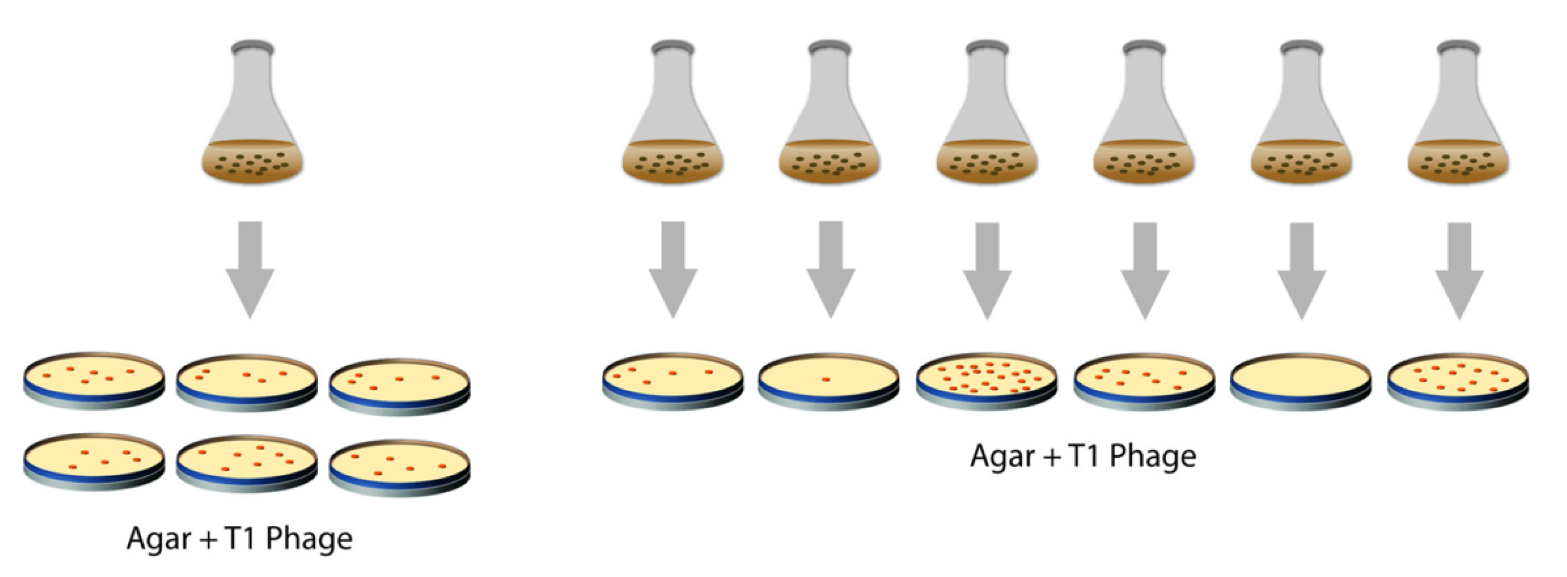
After designing and performing the now-famous “fluctuation test” experiments, Luria enlisted the theoretical expertise of Max Delbrück, which resulted in their seminal paper [1]. Luria and Delbrück made a convincing case in favor of the spontaneous mutation hypothesis by showing that the experimental pattern of variability was inconsistent with directed mutation. They established that the number of mutant cells was not Poisson, but it is just as important to the story that they were unable to mathematically describe that non-Poisson distribution. It took six more years until Lea and Coulson found the probability-generating function of the mutant distribution [11]. This was followed by the work of many others who presented alternative proofs, studied the same question within different stochastic frameworks, proposed statistical treatments and alternative approaches to calculating mutation rates, and derived asymptotic results (see the excellent review by Zheng [12]).

While most biologists presumed that Luria–Delbrück dealt the death knell to Lamarckism, the specter of Lamarck has unfortunately re-arisen several times since their publication. Claims of directed mutation were made by Cairns, Overbaugh, and Miller [13], Sarkar [14], Hall [15], and Heidenreich [16], among others. Holmes et al. [17] argued that the original Luria–Delbrück data cannot rule out a model that favors both Darwinian and Lamarckian mechanisms.

A root reason for the controversy was the fact that investigators were initially flabbergasted by post-plating mutations. This phenomenon is quite easy to understand in light of the mutation-mutant principle [18,19]. After the dust settled, biologists were quite nonchalant about this sort of mutation. For example, Lang [20] used a two-parameter model to fit data, taking into account post-plating mutations. Additionally, Ford et al. [21] followed suit. Unaware of these developments, Holmes et al. [17] went the extra mile to prove something that biologists already regarded as mundane. A subtler reason for the persistent belief in Lamarckism is the fact that post-plating mutations (or mutations induced by drugs) tend to occur at higher rates, but Witkin [22] has emphasized that this phenomenon is unlikely to be evidence of Lamarkism. An account more accessible to biology students is the introductory section of [23] where Zheng has developed new computational methods that take into account the idea that “nonlethal exposure of antibiotics [can] increase rates of bacterial mutations …[and where] some wide-type cells may be killed by nonlethal exposure to an antibiotic, [whereas resistant] mutants proliferate unimpeded….”.

Renewed scrutiny has also led to questions about bacterial evolution in light of bacterial adaptations through the CRISPR-Cas viral defense system. This quasi-Lamarckian behavior, however, likely evolved by random mutations and natural selection, has led some to imagine an alternative scientific history that might have occurred if Luria and Delbrück had used for their experiment, not E. coli, in which the CRISP-Cas mechanism is suppressed, but another bacterial species, e.g., Streptococcus thermophilus in which it is not [24,25]. The authors challenge us to ask: Would they have found evidence in favor of the directed mutation hypothesis? How would that have affected the course of future discoveries? This “What if…” approach, they say, “underscores the fact that, like evolution, science perhaps also progresses both adaptively and randomly” [24]. Engaging mathematics students with these questions is an important step in the process. The story continues, and it matters.

2.2. The Experiment

To begin, Luria started a series of identical cultures of bacteria, each starting with very few bacteria, which he allowed to grow for approximately 24 h until each culture contained about a billion bacteria. Each culture was plated individually and mixed with the phage. After another 24 h, he counted the number of resistant colonies per plate to find that he had, on average, about ten per plate, but there were many plates without resistant colonies and a few with “jackpots,” showing a large difference between the plated cultures.

His control was to start a single culture from a few cells, wait for it to grow, divide it into small portions and plate each individual portion to mix with the phage. Then, as before, he counted the resistant colonies after 24 h. He observed that the average number of resistant colonies per plate was about 10 (just as in the previous experiment), but this time the individual numbers were randomly spread about the average, and there were no “jackpots” (Figure 2).

2.3. The Mathematics Curriculum

The Luria–Delbrück idea is brilliant in its simplicity: the pattern of variability in the number of mutant cells ought to differ under the competing hypotheses of spontaneous vs. directed mutations (Darwin vs. Lamark). When students understand this idea, they understand something much more general: variability is natural, quantifiable, and predictable. It cannot be eliminated or (in some cases) controlled, but it can be described, and studied mathematically.

It is way too often that standard courses in mathematics fail to underscore this. Courses such as Finite Mathematics or Discrete Mathematics often focus exclusively on estimating elementary probabilities through counting arguments in the context of games of chance (cards, dice, guessing games), and Introductory Statistics courses are concerned primarily with teaching students how to compute the average and standard deviation of data sets, compare between-groups proportions and averages, and assess linear dependencies between quantitative factors (linear regression). These are all worthy goals, but in many courses, the ideas are obscured in favor of rote memorization of formulas that many students do not understand. The approach by Tintle et al. [27] to teach elementary statistics by way of simulations and using authentic projects drawn from recent peer-reviewed publications (called by the authors “explorations”) is a notable exception and has been gaining popularity in recent years.

Dedicated higher-level Probability courses offer a much broader view of the discipline—the standard list of topics extends beyond combinatorial counting arguments and covers random variables, discrete and continuous distributions, marginal and conditional distributions, moment and probability generating functions, limit theorems, and (time permitting) the basics of stochastic processes. To the best of the authors’ knowledge, however, Luria–Delbrück’s work is not found in any of the standard probability texts, thus missing an opportunity to discuss the importance of sample variance as a distinguishing factor between different types of distributions.

Of course, the argument that there is only a certain amount of “material” such courses can cover is a valid one. What we argue here is that some of it, especially when presented in ways that provide little context for its importance in authentic settings, can be reimagined and introduced through the lens of Luria–Delbrück experiments and analyses. What is more, introducing their work in a probability course opens the door to have students continue developing the relevant mathematics in other courses such as Calculus, Differential Equations, Real Analysis, and Mathematical Modeling.

How to mathematically describe and quantify patterns of variability offers an opportunity to understand the value of using models, how models rely on assumptions, and how to test models by using simulations and experimental data. Calculus is not required for the discrete-time model. For students with a calculus background, familiarity with rates of change, infinite series, and conditional probability provides a bridge to more advanced mathematical treatments. It gives the necessary tools to determine the probability-generating function of the number of mutants under the spontaneous mutation hypothesis.

Below, we will outline the theory with plenty of mathematical detail, hoping that instructors will find it helpful in case they choose to adapt parts of the material as course modules. The LaTeX file can also be obtained from the authors upon request for classroom use and adaptation.

3. Mathematical Models

We first present the underlying mathematical model for discrete time, following closely the work of Baake [28], where the variance of the number of mutants can be computed exactly under each hypothesis. We follow up with a generalization to continuous time, which allows for computing the probability-generating function for the distribution of mutants obtained by Lea and Coulson [11].

3.1. The Luria–Delbrück Model with Discrete Time

With the assumption that time t is discrete ($t=0,1,2,\dots$), we think of synchronized cell division where a unit of time equals the time between cell divisions. Thus t counts the number of generations. Let $n\left(t\right)=2^t$ denote the number of cells produced by a single sensitive cell after time t ($n\left(0\right)=1$), and let T be the time when the phage is introduced. It is common to also set $N=n\left(T\right)=2^T$.

The main assumptions of the model are as follows:

• When a cell divides, a mutation may occur in one of the daughter cells with a small probability p ($p\approx 0$);
• At any time t, the number of mutated cells in the population is negligible in comparison with $n\left(t\right)$. This is justified since the mutation probability p is small;
• Mutations are independent, and both sensitive and mutant cells divide every generation;
• Backward mutations (from a resistant cell to a sensitive one) are negligible.

Before we proceed, a few comments are in order. Assumption 1 rules out the possibility of both daughter cells mutating when a cell divides. Since p is very small, the probability $p^2$ for this to occur is much smaller and can be ignored for the purposes of our discussion. That said, the reader may choose to consider Zheng [12] for a discussion of this possibility and the paper [29] by the same author for an alternative discrete-time model—the so-called Haldane model, developed around 1946.

Now let $Z=Z\left(T\right)$ be the number of resistant cells at time T. Our goal is to determine what properties Z would have under the directed and under the spontaneous mutation hypotheses.

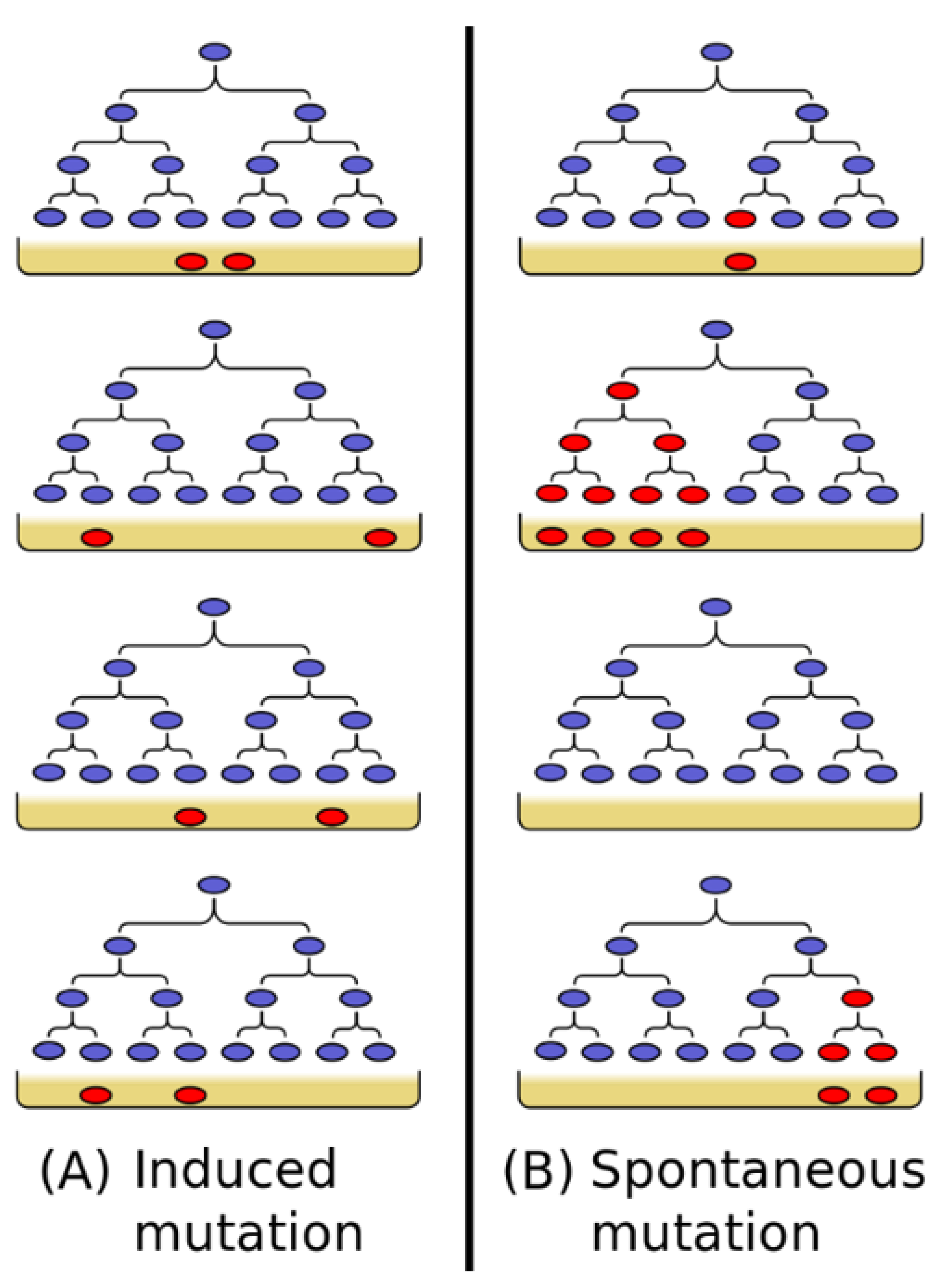
3.1.1. Case 1: Directed Mutations

In this case, each of the N cells in generation T mutates with probability p. Since mutation events are independent, the number of resistant cells has a binomial distribution with parameters N and p. Therefore,

$$\mathbb{E}\left(Z\right)=Np,\mathbb{V}\left(Z\right)=Np(1-p).$$

(1)

Since p is small, $1-p\approx 1$, and thus $\mathbb{E}\left(Z\right)\approx \mathbb{V}\left(Z\right)$, or, which is the same,

$$\frac{\mathbb{E}\left(Z\right)}{\mathbb{V}\left(Z\right)}\approx 1.$$

(2)

If we consider a Poisson approximation with parameter $\lambda =Np$ of the Binomial distribution of Z, then $\mathbb{E}\left(Z\right)=\mathbb{V}\left(Z\right)=\lambda$ and the ratio in Equation (2) is exactly 1.

3.1.2. Case 2: Spontaneous Mutations

In this case, calculating $\mathbb{E}\left(Z\right)$ and $\mathbb{V}\left(Z\right)$ requires more careful examination.

Let

$$X\left(t\right)=\mathrm{the}\mathrm{number}\mathrm{of}\mathrm{new}\mathrm{mutants}\mathrm{that}\mathrm{appear}\mathrm{at}\mathrm{time}t$$

and

$$\begin{array}{cc}\hfill Y_T\left(t\right)=& \mathrm{the}\mathrm{number}\mathrm{of}\mathrm{resistant}\mathrm{cells}\mathrm{at}\mathrm{time}T\hfill \\ & \mathrm{that}\mathrm{are}\mathrm{offspring}\mathrm{of}\mathrm{a}\mathrm{cell}\mathrm{mutated}\mathrm{at}\mathrm{time}t<T.\hfill \end{array}$$

Since $Y_T\left(t\right)=0$ for $t\ge T$, a mutation happening at time t will have $2^{T-t}$ offspring at time T, leading to

$$Y_T\left(t\right)=X\left(t\right)2^{T-t}.$$

(3)

The cumulative number of mutants at time T will then be

$$Z=\sum _{t=1}^T{Y}_T\left(t\right)=\sum _{t=1}^{T}Y\left(t\right).$$

(4)

In the second equality, we have simplified the notation, using $Y\left(t\right)$ for $Y_T\left(t\right)$ but we should keep in mind its dependence on T.

We now need to calculate the expected value and variance of Z, for which we need the expectations and variances of $X\left(t\right)$ and $Y\left(t\right)$.

Since p is small (Assumption 1), mutations are independent (Assumption 3), and the number of sensitive cells in the population is very close to $n\left(t\right)=2^t$ (Assumption 2), the number of new mutants at time t, $X\left(t\right)$, is approximately Binomial, and

$$\mathbb{E}\left(X\right(t\left)\right)\approx n\left(t\right)p,\mathbb{V}\left(X\right(t\left)\right)\approx n\left(t\right)p(1-p)=(1-p)\mathbb{E}\left(X\right(t\left)\right).$$

(5)

From Equation (3), for $1\le t\le T$ (and since $n\left(t\right)=2^t$),

$$\begin{array}{cc}\hfill \mathbb{E}\left(Y\right(t\left)\right)& =2^{T-t}\mathbb{E}\left(X\left(t\right)\right)=2^{T-t}n\left(t\right)p\hfill \\ \hfill & =\frac{2^T}{2^t}n\left(t\right)p=Np\hfill \end{array}$$

(6)

$$\begin{array}{cc}\hfill \mathbb{V}\left(Y\right(t\left)\right)& =2^{2(T-t)}\mathbb{V}\left(X\left(t\right)\right)\hfill \\ \hfill & =2^{2(T-t)}n\left(t\right)p(1-p)\hfill \\ \hfill & =2^{(T-t)}(1-p)\mathbb{E}\left(Y\left(t\right)\right)\hfill \end{array}$$

(7)

Consequently, the expected number of resistant cells when the virus is introduced at time T is

$$\mathbb{E}\left(Z\right)=\sum _{t=1}^T\mathbb{E}\left(Y\left(t\right)\right)=TNp$$

(8)

and

$$\begin{array}{cc}\hfill \mathbb{V}\left(Z\right)& =\sum _{t=1}^T\mathbb{V}\left(Y\left(t\right)\right)\hfill \\ \hfill & =\sum _{t=1}^T{2}^{T-t}(1-p)\mathbb{E}\left(Y\left(t\right)\right)\hfill \\ \hfill & =2^{T}Np(1-p)\sum _{t=1}^T{2}^{-t}\hfill \\ \hfill & =2^{T}Np(1-p)(1-\frac{1}{2^T})\hfill \\ \hfill & =(2^T-1)Np(1-p).\hfill \end{array}$$

(9)

Using once again than $1-p\approx 1$, and that $2^T$ is very large, we obtain that under the spontaneous mutation hypothesis

$$\frac{\mathbb{V}\left(Z\right)}{\mathbb{E}\left(Z\right)}\approx \frac{2^T}{T}\to \infty ,\mathrm{as}T\to \infty .$$

(10)

Thus, in that case, the ratio variance/expectation for the mutants will be much greater than 1.

3.2. The Luria–Delbrück Model with Continuous Time

The continuous model requires the use of calculus (rates of change, infinite series, differentiating infinite series) and is an excellent project for courses in calculus, calculusbased mathematical modeling, and real analyses. It will also be beneficial to students in Differential Equations courses, as the probability-generating function of Z is obtained as a solution of a differential equation.

To begin, just as in the discrete-time case, let $n=n\left(t\right)$ be the population size, grown from a single cell, at time t ($n\left(0\right)=1$), and let $Z=Z\left(t\right)$ be the number of mutant cells at time t. Let $\mathbb{E}\left(Z\right)$ and $\mathbb{V}\left(Z\right)$ denote the mean and the variance of Z.

When time is considered continuous, the model assumptions are as follows:

1’

The mutation rate is $\alpha$, meaning that a mutation of a sensitive cell may occur at any time $dt$ with probability $\alpha dt$ ($\alpha \approx 0$);

2’

At any time t, the number of mutated cells in the population is negligible in comparison with $n\left(t\right)$. This is justified since the mutation probability $\alpha$ is small;

3’

Sensitive cell numbers grow exponentially (and deterministically) at a rate $\beta$; that is

$$n=e^{\beta t}.$$

4’

Each mutant cell can split at time $dt$ into two mutant cells with probability $\beta dt$, independent of other cells. This probability is the same for all mutants and does not depend on the cell’s age. With this assumption, the number of mutant cells Z will always have an integer value. The splitting rate $\beta$ is the same as the growth rate of sensitive cells.

5’

Backward mutations (from a resistant cell to a sensitive one) are negligible.

Note that assumptions 2’ and 5’ are the same as in the discrete-time case, while assumptions 1,’ 3’, and 4’ are modifications of those in the discrete-time model.

With these assumptions, we follow the work of Lea and Coulson [11]. The difference with the original 1943 Luria–Delbrück model is that Luria and Delbrück assumed deterministic exponential growth of rate $\beta$ for both populations—the population of sensitive bacteria and the population of mutants. In contrast, Lea and Coulson made the additional assumption 4’ that would allow us, as we will see below, to determine the probability-generating function of the number of mutants Z. The paper by Armitage [30] contains more details, as well as an interesting history of prior work. (Those familiar with stochastic processes will recognize that 4’ assumes that the growth of mutant cells follows a Yule stochastic birth process with birth rate $\beta$. For very large t, $Z\left(t\right)$ is well approximated by $e^{\beta t}$, which is what Luria and Delbrück assumed. See the Discussion section for how this may be a pathway to initiating student research projects on random processes).

We should also note that, in principle, both $\beta$ and $\alpha$ may depend on t. In their work [11], Lea and Coulson make the observation that even though $\alpha$ and $\beta$ may change with time, it would make sense to assume that $\alpha$ and $\beta$ are affected similarly by factors such as nutritional conditions and population density. Thus, they make an additional assumption that the mutation rate per generation $\alpha /\beta$ (though not per unit time) may be considered constant even though $\alpha$ and $\beta$ are not.

Just as in the discrete-time model, we will now compute the ratio of $\mathbb{E}\left(Z\right)$ and $\mathbb{V}\left(Z\right)$ under the directed and spontaneous mutation hypotheses. We then follow the work by Lea and Coulson [11] to determine the probability-generating function of Z.

Consider again the population of size $n=n\left(t\right)$. Assumption 3’ now implies,

$$dn=n\beta dt,\mathrm{or},\mathrm{equivalently},\beta dt=\frac{dn}{n}.$$

(11)

Since $\alpha$ is the mutation rate, the average number of mutations in a population of size n in time $dt$ is $n\alpha dt$. Here, we use Assumption 2’, which allows us to use the total number of organisms $n\left(t\right)$ and not subtract the number of mutants. Thus, the average number of mutations to occur by the time the population has grown to size $n=n\left(t\right)$ is

$$m={\int }_0^{t}n\alpha dt=\frac{\alpha }{\beta }{\int }_1^{n}dn=\frac{\alpha }{\beta }(n-1)\approx \frac{\alpha }{\beta }n.$$

(12)

Let us now denote, for $r=0,1,2,\dots ,$

$$p_r=p_r\left(t\right)=P\left(\mathrm{a}\mathrm{culture}\mathrm{of}\mathrm{size}n\mathrm{has}r\mathrm{mutant}\mathrm{bacteria}\mathrm{at}\mathrm{time}t\right)=P\left(Z\left(t\right)\right)=r.$$

(13)

In what follows, we should suppress the dependence on time in the notation but should remember that n, $p_r$, and Z depend on t and $\alpha /\beta$ is constant.

3.2.1. Case 1: Directed Mutations

Let us assume the phage was introduced at time T when the population has size $N=n\left(T\right)$. Just as in the discrete-time case, each of the N cells can, at time [T, $T+dt$], mutate with probability $\alpha dt$. Since mutation events are independent, the number of resistant cells has Binomial distribution with parameters N and $\alpha dt$, which can be approximated using a Poisson distribution with mean and variance $\alpha$. Therefore,

$$\mathbb{E}\left(Z\right)=\alpha ,\mathbb{V}\left(Z\right)=\alpha ,\mathrm{and}\mathrm{thus}\frac{\mathbb{V}\left(Z\right)}{\mathbb{E}\left(Z\right)}=1.$$

(14)

3.2.2. Case 2: Spontaneous Mutations

Consider a culture of size $n=n\left(t\right)$ with r mutants. The proportion of mutants at this time is $p_r$. How can it change in time $dt$? That is, what is the proportion of mutants at time $t+dt$?

Consider

$$p_r+d{p}_r=p_r+\frac{d{p}_r}{dn}dn,$$

the probability that the number of mutants in a population of size $n+dn$ is r. This can happen in the following ways for $r\ge 1$:

(a)

At time t, the culture had $r-1$ mutants, and one of them divides at time $dt$. The probability of this event is

$$p_{r-1}(r-1)\beta dt=p_{r-1}(r-1)\frac{dn}{n};$$

(b)

At time t, the culture had $r-1$ mutants and a mutation occurred at time $dt$. The probability of this event is

$$p_{r-1}\alpha ndt=p_{r-1}\frac{\alpha }{\beta }dn;$$

(c)

At time t, there were r mutants, and neither a division nor a mutation occurred at time $dt$. The probability of this event is

$$p_r(1-\alpha ndt-r\beta dt)=p_r(1-r\frac{dn}{n}-\frac{\alpha }{\beta }dn).$$

Combining (a)–(c) gives the following equations:

$$p_r+d{p}_r=p_{r-1}[(r-1)\beta +\alpha n]dt+p_r[1-r\beta +\alpha n]dt.$$

(15)

Simplifying yields

$$\frac{d{p}_r}{dt}=p_{r-1}[(r-1)\beta +\alpha n]-p_r[r\beta +\alpha n].$$

(16)

Rearranging, and recalling, from Equations (11) and (12) that

$$\beta dt=\frac{dn}{n},\mathrm{and}m=\frac{\alpha }{\beta }n,$$

we obtain

$$\frac{d{p}_r}{dm}+p_r+p_r\frac{r}{m}=p_{r-1}(1+\frac{r-1}{m}).$$

(17)

We will now use Equation (16) to obtain $\mathbb{E}\left(Z\right)$ and $\mathbb{V}\left(Z\right)$ and Equation (17) to obtain the probability generating function of Z.

Expected value and variance of the number of mutants Z. Note that

$$\frac{d}{dt}\mathbb{E}\left(Z\right)=\sum _{r=1}^{\infty }r\frac{d{p}_r}{dt},$$

and so, multiplying Equation (16) by r and taking the sum over r, we obtain

$$\begin{array}{cc}\hfill \frac{d}{dt}\mathbb{E}\left(Z\right)& =\sum _{r=1}^{\infty }r[\beta (r-1)p_{r-1}-\beta r{p}_r+\alpha n{p}_{r-1}-\alpha n{p}_r]\hfill \\ \hfill & =\beta \underset{\mathrm{I}}{\underbrace{{\displaystyle \sum _{r=1}^{\infty }}r(r-1)p_{r-1}}}-\beta \underset{\mathrm{II}}{\underbrace{{\displaystyle \sum _{r=1}^{\infty }}{r}^2{p}_r}}+\alpha n\underset{\mathrm{III}}{\underbrace{{\displaystyle \sum _{r=1}^{\infty }}r{p}_{r-1}}}-\alpha n\underset{\mathrm{IV}}{\underbrace{{\displaystyle \sum _{r=1}^{\infty }}r{p}_r}}.\hfill \end{array}$$

(18)

With the understanding that for any $r<0$, $p_r=0$, for the sum denoted as I, we obtain:

$$\begin{array}{cc}\hfill \sum _{r=0}^{\infty }r(r-1)p_{r-1}=\sum _{r=0}^{\infty }(r+1)r{p}_r& =\sum _{r=0}^{\infty }{r}^2{p}_r+\sum _{r=0}^{\infty }r{p}_r\hfill \\ \hfill & =\mathbb{E}\left(Z^2\right)+\mathbb{E}\left(Z\right).\hfill \end{array}$$

(19)

For sum III,

$$\begin{array}{c}\hfill \sum _{r=0}^{\infty }r{p}_{r-1}=\sum _{r=0}^{\infty }(r-1)p_{r-1}+\sum _{r=0}^{\infty }{p}_{r-1}=\mathbb{E}\left(Z\right)+1.\end{array}$$

(20)

Sum II gives $\mathbb{E}\left(Z^2\right)$ and sum IV is $\mathbb{E}\left(Z\right)$. Combining back into Equation (18) we obtain the following differential equation for $\mathbb{E}\left(Z\right)$:

$$\frac{d}{dt}\mathbb{E}\left(Z\right)=\beta \mathbb{E}\left(Z\right)+\alpha n=\beta \mathbb{E}\left(Z\right)+\alpha e^{\beta t}.$$

(21)

Solving leads to

$$\mathbb{E}\left(Z\right)=\alpha t{e}^{\beta t}.$$

(22)

To find $\mathbb{V}\left(Z\right)=\mathbb{E}\left(Z^2\right)-{\left(\mathbb{E}\left(Z\right)\right)}^2$, we need to find $\mathbb{E}\left(Z^2\right)$. Multiplying Equation (16) now by $r^2$ and applying the same approach, we obtain the following differential equation for $\mathbb{E}\left(Z^2\right)$:

$$\frac{d}{dt}\left(\mathbb{E}\left(Z^2\right)\right)=2\beta \mathbb{E}\left(Z^2\right)+\beta \mathbb{E}\left(Z\right)+2\alpha n\mathbb{E}\left(Z\right)+\alpha n.$$

(23)

Plugging in again $n\left(t\right)=e^{\beta t}$ and solving, yields

$$\mathbb{E}\left(Z^2\right)=\frac{\alpha e^{\beta t}}{\beta }(2e^{\beta t}-\beta t-2)+{\left(\mathbb{E}\left(Z\right)\right)}^2,$$

leading to

$$\mathbb{V}\left(Z\right)=\frac{\alpha e^{\beta t}}{\beta }(2e^{\beta t}-\beta t-2)=\frac{2\alpha e^{2\beta t}}{\beta }+o\left(e^{2\beta t}\right),$$

(24)

where $o\left(e^{2\beta t}\right)$ indicates terms that grow much slower with time than $e^{2\beta t}$. Combining with Equation (22) shows that

$$\mathbb{V}\left(Z\right)\approx \frac{2e^{\beta t}}{\beta t}\mathbb{E}\left(Z\right),$$

(25)

and

$$\frac{\mathbb{V}\left(Z\right)}{\mathbb{E}\left(Z\right)}=\frac{2e^{\beta t}}{\beta t}\to \infty ,\mathrm{as}t\to \infty .$$

(26)

Thus, under the spontaneous mutation hypothesis, the variance in the number of mutants is much bigger than the expected value.

The Probability Generating Function (PGF) of Z. Using the expression for probabilities $p_r$ from Equation (17), Lea and Coulson obtained the PGF $F(x,m)$ defined by

$$F(x,m)=\mathbb{E}\left(x^Z\right)=\sum _{r=0}^{\infty }{p}_r{x}^r,$$

(27)

where m is the average number of mutations when the population size is n. Then

$$\frac{\partial F}{\partial x}=\sum _{r=0}^{\infty }r{p}_r{x}^{r-1}\mathrm{and}\frac{\partial F}{\partial m}=\sum _{r=0}^{\infty }{x}^r\frac{d{p}_r}{dm}.$$

(28)

Multiplying Equation (17) by $x^r$ and summing up, gives

$$\sum _{r=0}^{\infty }{x}^r\frac{d{p}_r}{dm}+\sum _{r=0}^{\infty }{x}^r{p}_r+\frac{x}{m}\sum _{r=0}^{\infty }{x}^{r-1}r{p}_r=x\sum _{r=0}^{\infty }{x}^{r-1}{p}_{r-1}+\frac{x^2}{m}\sum _{r=0}^{\infty }(r-1)x^{r-2}{p}_{r-1},$$

(29)

which leads to

$$\frac{\partial F}{\partial m}+F+\frac{x}{m}\frac{\partial F}{\partial x}=xF+\frac{x^2}{m}\frac{\partial F}{\partial x}.$$

(30)

Thus, the PGF $F(x,m)$ satisfies

$$m\frac{\partial F}{\partial m}=m(x-1)F+\frac{\partial F}{\partial x}(x^2-x)m,\mathrm{with}F(0,m)=p_0=e^{-m},$$

(31)

where $p_0$ is the probability of having no mutant cells in a population of size $n=n\left(t\right)$.

Lea and Coulson went on to show that

$$F(x,m)={(1-x)}^{\frac{m(1-x)}{x}}.$$

(32)

was a solution to Equation (31), which can be checked by substitution.

3.3. Determining the Mutation Rate

It is interesting that eighty years after the publication of the Luria–Delbrück work, it is better known not for demonstrating that experimental data conforms with the spontaneous mutation hypothesis but rather for presenting an ingenious way for estimating the mutation rate. The paper [1] presents two such methods—the so called $p_0$-method and the method of likely averages. Significant progress has been made on this front since the original Luria–Delbrück work, and many more modern and more accurate methods have been developed in the past 80 years. Better methods have been necessary for two reasons. On one hand, some of the methods rely on mathematical assumptions that may be difficult to justify or verify in practice. On the other, experimental difficulties that impact accuracy should be considered. The need to develop reliable, easy-to-use approaches to estimating mutation rates has generated considerable literature on the subject, and the excellent reviews by Zheng [31], and Łazowski [32] outline the evolution of protocols for estimating mutation rates, providing the theoretical underpinnings of multiple methods together with some practical challenges related to their use.

In what follows, we focus on three classical methods: the two originally proposed in [1], and a method by Drake [33], based on the rate of growth of the average number of mutants $\rho =\mathbb{E}\left(Z\right)$ from Equation (21). The method of likely averages and Drake’s method are now outdated and should no longer be used in practice. We chose to present them here due to their historical significance, even though, from the very beginning, their use has been riddled with conceptual, experimental, and computational difficulties. In addition, many other methods can be traced back to them, and, for students, the history here is yet another powerful example of the idea that mathematical models inform experimental biology in important ways but that translations into practice may not be straightforward. The work by Zheng [31] could be used as a bridge to student research projects on the topic.

Nowadays, maximal (ML) methods are the predominant methods for estimating mutation rates in research. Describing those methods is beyond the scope of this work, but we should mention that several computational tools implementing various methods have been developed in the last decade and are freely available. The web-based webSalvador [34] (descending from rSalvador [35]) is perhaps the easiest to use. New statistically rigorous methods using Bayesian and Markov Chain Monte Carlo approaches have also been developed recently [36].

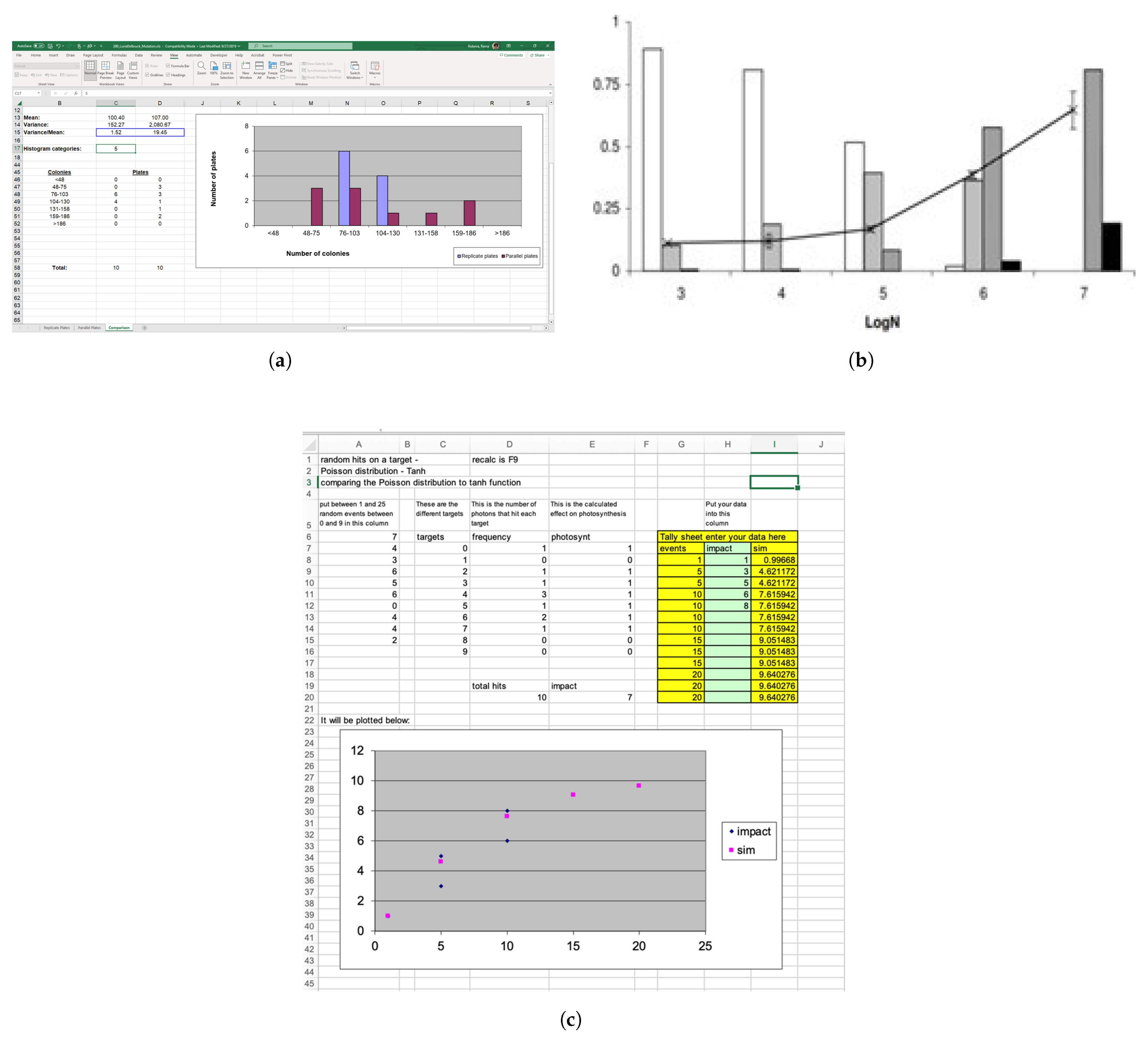
3.3.1. Method 1—Using a Poisson Approximation (The $P_0$-Method)

This method is the one biology students would most commonly learn about in the lab. Using the same notation as Equation (13), we let $p_0$ denote the probability that no mutations have occurred over the interval $[0,t]$ (no mutations in a population of size n). Since the number of new mutants over the interval [0,t] is Poisson with parameter m,

$$p_0=e^{-m}=e^{-\frac{\alpha }{\beta }n}$$

(using $m=\frac{\alpha }{\beta }n$, Equation (12)). Experimentally, this same probability $p_0$ may be approximated as the fraction of cultures showing no mutations in a large series of similar cultures:

$$p_0\approx \frac{\mathrm{number}\mathrm{of}\mathrm{cultures}\mathrm{with}\mathrm{no}\mathrm{mutations}}{\mathrm{total}\mathrm{number}\mathrm{of}\mathrm{cultures}}.$$

(33)

With this approximation for $p_0$, the average number of mutants is

$$m\approx -ln\left(p_0\right),$$

which, combined with Equation (12), gives the needed approximation for the mutation rate $\alpha$

$$\alpha \approx -\frac{\beta ln\left(p_0\right)}{n},$$

(34)

where the growth rate $\beta$, the population size n, and the proportion of cultures with no mutations $p_0$ are known/determined from the experiment.

3.3.2. Method 2—Using a Likely Average

This method does not make any assumptions about the distribution of mutants Z and uses only the assumption 3’ of exponential growth.

Equation (22) shows that the average number of mutants increases more rapidly than the population size n. Experimentally, though, for small mutation rates, it would be very unlikely to have an early mutation in a single or a limited number of experimental cultures. Thus, experimental results would very likely generate smaller values than the theoretical value from Equation (22). In the unlikely occasion that a mutation did occur early, the experimental average would be much larger than this theoretical value. Luria and Delbrück wrote:

This situation is similar to the operation of a (fair) slot machine, where the average return from a limited number of plays is probably considerably less than the input, and improbably, when the jackpot is hit, the return is much bigger than the input [1].

As we saw in Equation (24), this leads to what Luria and Delbrück called “an abnormally large variance” and note that for “such distributions, the averages derived from limited numbers of samples yield very poor estimates of the true averages.” To mitigate this situation, they proposed that, for a limited number of samples, it would be more appropriate to calculate the likely average r of the number of resistant bacteria

$$r=(t-t_0)\frac{\alpha }{\beta }n,$$

(35)

obtained by integrating Equation (21) over an interval $[t_0,t]$ (instead of $[0,t]$, which led to Equation (22)).The time $t_0$ should be such that prior to it mutations would be unlikely to occur in any of the experimental samples.

Luria and Delbrück chose $t_0$ to be such that up to that time, only one mutation has occurred on average in a group of C similar cultures. Integrating over $[t_0,t]$, similarly to Equation (12), we obtain

$$1=\frac{\alpha }{\beta }Cn\left(t_0\right),\mathrm{or}n\left(t_0\right)=\frac{\beta }{\alpha C}.$$

(36)

We may also connect $n\left(t_0\right)$ with $n=n\left(t\right)$, the number of bacteria at the time of observation, using that the population grows exponentially:

$$n=n\left(t_0\right)e^{\beta (t-t_0)},\mathrm{or}n\left(t_0\right)=n{e}^{-\beta (t-t_0)}.$$

(37)

Equating the two different representations of $n\left(t_0\right)$ from Equations (36) and (37), and solving for $t-t_0$ gives

$$t-t_0=\frac{1}{\beta }ln\left(\frac{\alpha }{\beta }nC\right).$$

(38)

With this, Equation (35) becomes

$$r=\frac{\alpha }{{\beta }^2}nln\left(\frac{\alpha }{\beta }nC\right).$$

(39)

Since the quantities r, $n=n\left(t\right)$, $\beta$, and C can be measured experimentally, Equation (39) can now be solved numerically to find the mutation rate $\alpha$.

3.3.3. Method 3—The Drake Equation

This method, proposed by Drake [33], uses Equation (21) to derive the rate of change of the proportion f of resistant mutants in the population.

Recall that (Equation (11)) $n\beta dt=dn$. With this, Equation (21) becomes

$$\frac{d\rho }{dn}=\frac{\alpha }{\beta }+\frac{\rho }{n},\mathrm{or},\mathrm{equivalently}d\rho =\frac{\alpha }{\beta }dn+\frac{\rho }{n}dn.$$

(40)

Consider now the fraction f of resistant mutants when the population size is n.

$$f=\frac{\rho }{n}$$

Then $\rho =fn$ and, by the product rule,

$$d\rho =fdn+fdn.$$

Replacing $d\rho$ in Equation (40) with this expression, simplifying, and dividing by $f=\rho /n$, leads to

$$df=\frac{\alpha }{\beta }\frac{dn}{n}.$$

Integrating this over a time interval $[t_0,t]$ gives

$$f-f_0=\frac{\alpha }{\beta }(ln\left(n\right)-ln\left(n_0\right))=\frac{\alpha }{\beta }ln(n/n_0),$$

(41)

and the mutation rate $\alpha$ can be estimated as

$$\alpha =\beta \frac{f-f_0}{ln(n/n_0)}.$$

(42)

Several comments are in order:

• Note that if we choose $t_0=0$ and assume, as we assumed before, $n\left(0\right)=1$ and $f_0=0$, Equation (42) yields

  $$\alpha =\beta \frac{f}{ln\left(n\right)}.$$
• Alternatively, to avoid the same type of problems as we discussed when describing Method 2 above, $t_0$ may be chosen so that $n_0=n\left(t_0\right)$ is the size of the culture when the first mutant appears. At that time, $n_0\approx 1/(\alpha /\beta )$, and $f_0$ is very small and can be ignored. Replacing this value for $n_0$ in Equation (41) and using that $f=\rho /n$, gives the following equation for the mutation rate:

  $$\frac{\rho }{n}=\frac{\alpha }{\beta }ln(\frac{\alpha }{\beta }n).$$

  (43)

The three methods presented here lay a foundation for many modifications. The works by Foster et al. [37], Zheng [31], and Łazowski [32] can be used as a launchpad for further investigations.

4. Suggestions for Classroom Use

In this section, we comment on ways to incorporate elements from this theory in several standard undergraduate mathematics courses. With some careful scaffolding, the discrete-time model could be used as a student project in some biology courses as well, e.g., genetics, ecology, evolution, developmental biology, and physiology.

4.1. Possible Uses of the Discrete-Time Model in Mathematics Courses

Except for Equation (10), the discrete-time model does not rely on calculus, and the use of limits in it may be easily avoided by examining the ratio $(2^T-1)/T$ for growing values of T to observe that it increases without a bound away from 1. Thus, in our view, this model could be incorporated into precalculus-level courses (e.g., Finite Mathematics, Discrete Mathematics, Mathematical Modeling) with the following scaffolding: (1) Rely on students’ intuitive understanding of Independence, (2) Outline the framework within which the Binomial distribution forms (a fixed number of independent trials is performed; each trial has only two possible outcomes—usually termed “success” and “failure”, and the probability for success is the same for all trials), and (3) Accept (perhaps after examining some examples) that when random quantities are independent, the variance of their sum is the sum of the variances as in Equation (9). We consider this an efficient way to bypass some technicalities that are of secondary importance to students with yet undeveloped mathematical maturity and show how the Binomial distribution can be used to generalize many of the combinatorial examples students encounter in these courses. With this, Equation (10) also provides an opportunity to use the closed form of a geometric sum, something they have likely already seen in problems focused on the growth of investment with compound interest-type problems.

In dedicated Probability courses, the scaffolding would be unnecessary, and this Luria–Delbrück model could be used with full mathematical justification. It may also be assigned as an independent project where students read the Braake paper [28], discuss it with their instructor, and write a paper or give a presentation on the topic.

Students who have taken calculus can be assigned a project to show that the binomial distribution $\mathcal{B}(N,p)$ obtained for the number of mutants under the directed mutations hypothesis is well approximated by a Poisson distribution $\mathcal{P}\left(\lambda \right)$, where $\lambda =Np$ remains constant when $N\to \infty$. As this fact is a standard material included in a calculus-based probability course, the Luria–Delbrück experiments can be used as an authentic example and as a way to justify why counts of “rare” events over a unit of time or space generally follow Poisson distribution laws. Those students may also be asked to compare the expressions for the ratios of the variants and the expected value in the discrete and continuous cases (Equations (10) and (26)) and comment on the comparison.

4.2. Possible Uses of the Continuous-Time Model in Mathematics Courses

Clearly, the model with continuous time requires some sophisticated mathematical treatment, but we hope that the outline presented here underscores its accessibility to students in calculus and in more advanced calculus-based courses. The first author, who used parts of this material in an advanced probability course, was able to observe genuine student interest once they got engaged with the project, even though their initial knowledge of biology was not strong. It improved while students worked on the project, but overall remained limited, which emphasizes the idea that understanding the importance of the questions raised and answered by Luria and Delbrück are easily understandable even for mathematics audiences with only limited background in biology. Additional observations include the following:

• Most students in the sciences are keenly aware of the ongoing political debates about evolution and how school boards nowadays may mandate that teaching evolution in the schools should necessarily be paired with “-parallel” theories, e.g., Lamarckism and intelligent design. To see how, at least in the bacterial world, it can be established that the directed mutations hypothesis is not supported by experimental data provides a high-impact example of the value of hypothesis-driven research.
• The fluctuation test allows students to see a statistical approach not based on comparing group proportions or means (which is almost exclusively what most introductory statistics courses do) and focusing instead on their variances. A discussion asking why averages do not allow for distinguishing between the hypotheses of spontaneous mutations and directed mutations provides an excellent opportunity to build a better understanding of how randomness is quantifiable.
• Most standard courses in mathematical modeling place emphasis on describing the time evolution of systems comprising interacting components through difference or differential equations; that is, using a deterministic approach. In rare cases when some stochasticity is added to the models, it is primarily in assuming that the values of the model parameters are drawn from an underlying distribution of interest (e.g., in the context of looking into a solution’s stability without performing full mathematical analyses). The fluctuation test uses a mathematical model very different from those they may have seen in such courses and, thus, presents an opportunity to broaden the scope of modeling approaches students are exposed to.
• There are many links relating the theory above to standard material taught in other courses. As an example, students in a probability class are introduced to probabilitygenerating functions, but justifying the term-by-term differentiation of the infinite series from Equation (28) is something that they will encounter in Calculus or Real Analysis courses. Verifying that the limit, as $x\to 0$, of the solution $F(x,m)$ in Equation (32) agrees with the condition $F(0,m)=p_0=e^{-m}$ is another good calculus problem. The use of “little o” notation in Equation (24) is an opportunity to talk about rates of growth at infinity.
• Changing the summation index in Equations (19) and (20) is something that comes up often in Differential Equations courses in the context of finding solutions in the form of infinite series—something students generally struggle with. In a Differential Equations course, it would also be of interest to ask students to obtain Equation (21) in an alternative way, without using assumption 4’ and the probabilities $p_r$. Instead, they may assume that the population of mutant cells grows exponentially at a rate $\beta$, just as the population of sensitive cells does (assumption 3’). To do that, they should notice that the rate of growth of $\rho =\mathbb{E}\left(Z\right)$ has two components: (1) a contribution from new mutations in time $dt$: $\alpha ndt$, and (2) a contribution from the growth of resistant mutants in time $dt$: $\beta \rho dt$. Thus, the rate of increase of the average number of resistant mutant bacteria is

  $$\frac{d\rho }{dt}=\alpha n+\beta \rho ,$$

  (44)
  providing an intuitive interpretation of Equation (21).
• Once students feel comfortable with the theory outlined above, there are many possible directions for student research projects. They can follow, e.g., the work of Ma [38] to analyze the distribution of mutant cells using discrete convolution powers or read Pakes’s [39] and Kemp’s [40] remarks on the Luria–Delbrück’s distribution to discover more of its mathematical properties, including asymptotic evaluations of the probabilities $p_r$. The short communication by Goldie [41] suggests an alternative method for finding the PGF $F(x,m)$ and the asymptotics of the probabilities $p_r$ by representing the number of mutant cells Z as a Poisson compound. Examining additional methods for estimating mutation rates, using [37] as a starting point is another possibility.
• If one is interested in more recent mathematical developments, the paper by Zheng in Chance [42], written for a general audience, can be used as a continuation of our Section 2.1. This pleasant read addresses the time span between the publications of the Luria–Delbrück paper [1] and that by Lea and Coulson [11], discussing unpublished efforts and anecdotes. This is followed by descriptions of more recent work on the topic. The review paper by the same author [12] provides a rigorous review of the mathematical literature until 1999, which will be of interest to those who pursue research in the field.
• A fine distinction of interest based on the assumptions under which the models are developed can be studied by the work of Luria–Delbrück [1], Lea and Coulson [11] and M.S. Bartlett. As mentioned earlier, Luria and Delbrück assumed deterministic growth of the sensitive and the mutant cells, while Lea and Coulson used a deterministic growth for the sensitive cells but assumed the growth of mutants followed a Yule branching process. Bartlett on the other hand, treats the growth of both sensitive cells and mutant cells as Yule processes. See [12,43] for the interesting history behind Bartlett’s work and references to it.
• Finally, it is important to help students realize that mathematical models for biology and medicine rely on assumptions that should be considered and weighed with great care. Due to those assumptions, mathematical models generally present useful but incomplete descriptions of cellular and molecular mechanisms. Students should be aware of the risks of drawing dubious conclusions based on simplifications that are more about mathematical tractability than about biological reality. There are certain mutations that are extremely hard to predict but can have significant biological consequences (see e.g., [44,45]). The accurate modeling of such processes may require different approaches or new mathematical treatments, thus advancing research in both mathematics and biology.

Our lists here present just a small portion of the many possible ways the Luria–Delbrück work links with topics in the standard mathematics curriculum and can be a springboard to student research where students could delve into the theory of stochastic processes. It is an example that shows how theoretical mathematics can be used to answer questions of clear practical importance to biology (something rare for advanced mathematics courses) while also propelling advancements in mathematical theory. In that sense, the fluctuation test is an example that will “keep giving,” as long as it appears on our radar. We hope this article makes a first step in assisting readers with this goal.

5. Educational Simulations, Mathematical Manipulatives, and Wet Laboratories

As mentioned already, notions of randomness are frequently counterintuitive and difficult for many students and present a special challenge for undergraduate biology education. The quantitative reasoning issue has been specifically addressed by Robson and Burns [46], and Meneely [47] focused on developing a primer on the Poisson statistical test. Here we highlight a few resources that can be used as hands-on activities geared at helping students with limited mathematical backgrounds to understand randomness, variability, rates of occurrence, and Poisson distributions in an applied context. These can prepare students for appreciating and better understanding the Luria–Delbrück idea for estimating mutation rates.

5.1. Simulations

Computer simulations are useful for a multitude of reasons. First, most mathematics students are unfamiliar with analyzing actual data from experiments and then exploring what would happen if the results were a little different. By varying entries in a spreadsheet or other interface, students often experience surprise when something counterintuitive to their expectation occurs [48]. Second, students can explore the differences among hypothesis-free exploration and model-using, model-revising, and model-building simulations. Thus, some simulations are black-box, and others are glass-box where the underlying mathematics is both accessible and visualizable. Furthermore, students who build simulations (“no-box”) benefit from translating a model to deal with actual data, units (dimensions), and visualization comprehensible to a user other than themselves [48]. These skills are frequently transferable to other contexts as well. Third, simulations also require students to think out the issues of dealing with continuous models in a discrete environment or actually transforming their model to a discrete version in the first place [49]. Too many students have only been used to dealing with ordinary differential equation and partial differential equation models and have no experience with finite difference equations and extensive use of iteration and recursion. Fourth, the visual interface of simulations is also crucially important to developing students understanding. For example, in the case of the distribution of univariate data, violin plots may be very preferable to box and whiskers displays because some non-Gaussian distributions are not bell shaped, and it is easier to see where the mean, median, and mode are distinctly different from one another [50]. See our earlier Section 3.3.2—Using a Likely Average, where we discuss the importance of assumptions about relationships between experimental averages and theoretical values. In the educational literature on visualization in computer simulations, seven I’s are cited as skills that are important: (1) illustrating; (2) informing; (3) integrating; (4) implicating; (5) inferring; (6) interpreting; and (7) illusions (perceiving ambiguity, complexity, alternatives, etc.) [51].

Weisstein, Jungck, and Green (https://bioquest.org/esteem/esteem_result.php accessed on 15 January 2023), and Carvajal-Rodríguez [52] have developed software simulations to engage students in understanding these quantitative ideas (Figure 3). In as much as the ESTEEM module is a spreadsheet, students could enter data from actual lab experiments, from the literature, or explore the impact of changing raw data to see what happens.

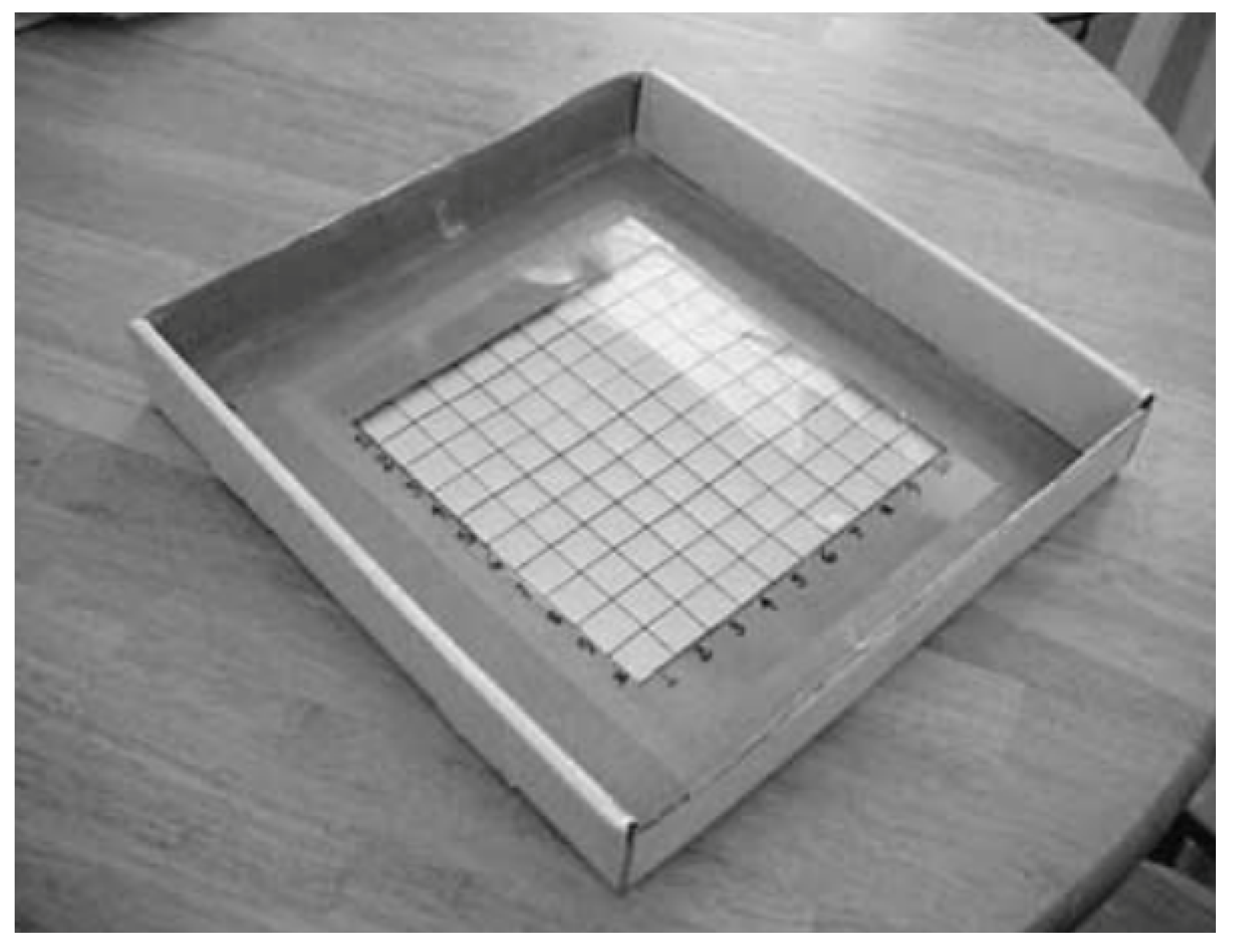
5.2. Mathematical Manipulatives

Manipulatives alone do not work well unless students are actively engaged in four different processes: (1) Starting out with very different conditions and exploring multiple iterations. (2) Graphing data in multiple ways. For example, by plotting a cobwebbing graph of successive values of $x_{t=n}$ versus $x_{t=n+1}$, there is a potential to discriminate between a highly regular pattern, and a chaotic process [53]. (3) Explicitly relating the component manipulatives to variables in the mathematical model. (4) Explicitly relating the component manipulatives to biological entities and processes (e.g., photons hitting chloroplasts in cells of a leaf). A teacher usually achieves success when students are using a manipulative model when they report counterintuitive results, express surprise, and actively start changing the game or activity to correspond with their ideas about what is happening in the natural physical system.

Furner and Worrell [54] state several important precautions about using manipulatives to engage students in developing conceptual ties from the analog world to theoretical models:

Teachers need to learn how to encourage student exploration, related discussion, and reflection about the prospective math concept they teach. They need to be comfortable with students’ exploration of the math concepts and possibly wandering off the ‘correct’ track or even to represent quantities in real-world contexts, challenging the teachers’ own mathematical viewpoint. Teachers cannot assume that when students use manipulatives they will automatically draw the correct conclusions from them … Teachers need to keep in mind that the student does not already possess this knowledge and still needs to make the correct connections between the manipulative and the underlying math concept. While math manipulatives are a valuable tool in the instruction of mathematics, teachers need to bridge the manipulatives to the representational and then abstract understanding in mathematics so that students internalize their understanding. Just using manipulatives by themselves without this may not have great value.

Furthermore, Ross-Hogaaboam-Gray and Hannay [55] emphasize that success in the use of manipulatives is strongly associated with both a teacher’s knowledge and confidence as well as a commitment to constructivist teaching.

Jungck, Gaff, and Weisstein [56] demonstrate the utility mathematical of manipulatives in helping students understand concepts like Poisson distributions. A specific application of Poisson distributions to photons impinging on the surface of a leaf and its relationship to photosynthesis was developed by Buonaccorsi and Skibiel [57] (Figure 4). They had students calculate: “(1) the observed frequencies of peas per quadrat, (2) the mean number of peas per quadrat, (3) the Poisson estimated probabilities for each outcome, (4) the Poisson expected frequencies, (5) the mean and variance of the distribution, (6) the coefficient of dispersion (CD) and (7) the fit of observed and expected frequencies using a chi-square goodness of-fit test.” In a similar fashion, Haddix and Danderson [58] developed a dice-roll exercise to simulate “the probability basis for mutation rate calculation.”

5.3. Wet Laboratories

Cornette et al. [59] pioneered the use of wet laboratories in a freshman calculus class. From analyzing whether the growth of mold on the surface of a cup of tea seasoned with sugar or a slice of bread in the refrigerator fit a linear, exponential, or logistic model to investigating sunlight depletion below the surface of a lake or ocean and its relationship to underwater photography to a standard biology laboratory osmosis experiment, they carefully developed relevant calculus models, used theorems in a way that students appreciated the generalization that extended well beyond individual cases, and how models grew in sophistication with each passing week. Note that their book is also available online as an Open Educational Resource. Subsequently, others adopted the use of labs in mathematics courses. Sanft and Walter [60,61] included four wet lab experiments on enzyme kinetics, blood glucose–insulin feed-back and homeostasis, population growth, and random walks/diffusion in their mathematical modeling course. They argue:

It is important to provide students in biology and mathematics with opportunities to interact and collaborate with one another. However, it can be a challenge to develop integrated courses that are accessible and useful to both sets of students. In this paper, we describe the development, implementation, and assessment of a team-taught course that was developed to provide undergraduate students with a truly integrated experience by incorporating a wet laboratory into a mathematics course …The wet laboratory in Math 236 enabled students to undertake experimentation, data collection, mathematical modeling, and statistical computation, all essential to developing models of biological processes. Each lab addresses core concepts in the categories outlined in BIO 2010 [2]: calculus, linear algebra, dynamical systems, computation, data structures, rate of change, modeling, equilibria and stability, structure, and interactions. Although each lab touches on each of these areas, the tools become more sophisticated as the semester progresses.

Not only do such courses address a national call for improving interdisciplinary mutual appreciation of mathematical and biological educators [62], but, more importantly, they make a significant difference in student learning [63].

Haddix, Paulsen, and Werner [64], Green and Bozzone [65], Robson and Burns [46], Hester, Sarvary, and Ptak [66], Smith, Golomb, Billstein, and Montgomery Smith [67], Amir and Balaban [68], and Hutchinson [69] have all published laboratory protocols for experimental investigations that lead to fluctuation tests on bacterial populations.

6. Why Measuring Mutation Rates Matters in Everyday Life

6.1. Radiation: Hiroshima/Nagasaki/Fukushima/Chernobyl/Three Mile Island

One way of inducing mutations is through ionizing radiation. As we write this article, we are concerned that with Ukraine under attack, the potential of a second Chernobyl-like event in that nation is a reality that endangers international world order and is threatening the lives of people in many nations. When the Three Mile Island accident happened in the United States, the only significant data on pre-accident radiation levels had been collected by students of Professor Priscilla Laws at Dickinson College in Pennsylvania. Thus, there is a precedent for students being engaged with such an important issue and making a difference.

After the atomic bombs destroyed Hiroshima and Nagasaki at the end of World War II, scientists studied the mutations that occurred in survivors over a long period. Prior to these bombings, Native Americans in the southwestern United States and New Zealand sailors were exposed to radiation during tests of the bomb prototypes and suffered serious health effects. Most recently, the tsunami that destroyed the Fukushima nuclear power plant again affected the lives of many survivors in the immediate area. Numerous reports on these incidents are available and could be used to develop a case with a lot of primary data.

As an additional motivator for students, Moller and Mousseau [70] make the case for why much more research is needed:

The disaster at the Chernobyl nuclear power plant in 1986 released 80 petabecquerels of radioactive cesium, strontium, plutonium, and other radioactive isotopes into the atmosphere, polluting 200,000 $k{m}^2$ of land in Europe. As we discuss here, several studies have since shown associations between high and low levels of radiation and the abundance, distribution, life history, and mutation rates of plants and animals. However, this research is the consequence of investment by a few individuals rather than a concerted research effort by the international community, despite the fact that the effects of the disaster are continent-wide. A coordinated international research effort is therefore needed to further investigate the effects of the disaster, the knowledge that could be beneficial if there are further nuclear accidents, including the threat of a ‘dirty bomb’.

Furthermore, Sacks, Meyerson, and Siegel [71] have argued that much of the prior work has used “specious statistics” because of a dependence on an old “linear no-threshold hypothesis (LNTH)” and their work has also been critiqued and extended. We believe that such controversy affords an additional opportunity for students to appreciate why mathematics can matter so much.

A case developed around nuclear warfare would have pleased Luria and Delbrück very much as Luria fled fascism in Italy and Delbrück fled Nazism in Germany to emigrate to the United States [9]. Once here, Luria was an activist concerned about racial segregation, eugenic discrimination, workers’ rights, academic freedom, and especially biological and nuclear weapons. Selya [72] obtained records from the FBI on Luria through the Freedom of Information Act that showed that Luria was carefully monitored and was thoroughly questioned about his colleagues and affiliations. At one time, Luria was denied a visa to travel to a scientific meeting and see his ill mother. As Abbott noted [73], “As Luria’s success grew, so did his political involvement.” Students frequently do not get the opportunity to see the human side of scientists and mathematicians and how their work relates to crucial issues in society. We believe that part of education is to prepare students for socially responsible use of the knowledge developed in our classes so that they are active participants in our democracy.

6.2. Cancer Chemotherapy—Evolution of Resistance

One of the unfortunate aspects of the education of physicians and the misinformation received by patients is the conceptual misunderstanding of evolution. The use of military metaphors such as the “war on cancer,” chemotherapeutics as attackers, strike forces, missiles, etc., cancer cells as enemies, and euphemisms such as the cancer returns or the battle has been lost divert attention from understanding that cancers involve a population of cells that have mutations that differentiate them from normal cells and natural selection will promote the survival of cells that outcompete other cells in acquiring nutrients and oxygen that promote their growth. Many patients, after surgery, chemotherapy, and nuclear therapy, experience a second round of cancerous growth due to the evolution of resistant cells being able to re-populate tissues. “The result is that virtually all cancer deaths are due to therapeutically resistant disease” [74]. Merlo et al. [75] state: “Cancer is a disease of clonal evolution within the body. This has profound clinical implications for neoplastic progression, cancer prevention, and cancer therapy.” Hence, many evolutionarily-informed physician researchers have argued that we need a “paradigm shift” in cancer research and treatment [62,76,77,78].

The fluctuation test has long been explicitly used in the cancer research literature (see, e.g., [79,80,81,82,83,84]). Two books that give a good foundation for undergraduates are Goldie and Coldman [85], who spend three chapters on the Luria–Delbrück distribution and differencing between directed and random mutation and Durrett [86] who develops results on continuous time branching processes and applies them to study the rate of tumor growth, extending the classic work on the Luria–Delbrück distribution. The probability that mutations that confer resistance to treatment are present at detection and quantifying the extent of tumor heterogeneity is also calculated. After Goldie and Coldman [85] discuss the classical experiments, they present an interesting hypothetical experimental model using Lederbergs’ replica plating technique where “the magnitude of experiments involved may make them impractical” but would easily be modeled mathematically by undergraduates. Cells are laid out on a rectangular grid so that the spatial coordinates of the microwells of cells are explicit. They set up the transfer of cells in subsequent generations such that: “Under the directed mutation model, there will be few surviving cells (resistant) at the same coordinates on each plate. Under the random mutation model, the possibility that resistance may have been pre-existing increases the probability that there will be resistant cells at the same locations.”

Goldie and Coldman’s work is critiqued in another accessible book edited by Pinedo and Giaccone [87]. Another alternative presented by Durrett [86] is to look at the reciprocal problem of the loss of resistance. Unfortunately, a major overview of drug resistance with 31 chapters only deals with molecular and physiological approaches [88] with no treatment of either mathematics or evolution, but the data therein could be used to develop models whose parameter estimates would be informed by experiments.

Six types of cancer evolution models are described by Zhu, Xu, and Luo [89]. However, here again students could explore a controversy started by Graham and Sottoriva [90], Turajlic et al. [91], and Saito et al. [92] who argue that models should include punctuated equilibria to understand evolution in cancer. Students could contrast their approach with the Fluctuation Analysis approach and models that consider most mutations to be neutral [93,94,95] rather than detrimental or beneficial. In this journal, we recommend that readers examine the work of Frank [96] and some of his previous work on the use of Luria and Delbrück on cancer (e.g., his brief communication on developmental predisposition to cancer [97] can be used to initiate interesting student research projects).

6.3. Antibiotic Resistance

In [98], Lesho and Laguio-Vila write:

Antimicrobial-resistant infections kill 700,000 patients every year …By 2050, they are projected to cause 10 million deaths per year at a cumulative global cost of $100 trillion. Professional societies and international health agencies, including the United Nations, have declared escalating antimicrobial resistance as one of the gravest and most urgent threats to global public health and issued calls for action.

Soon after Luria and Delbrück published their paper using bacteriophage as a selective agent, biologists started applying the Fluctuation Test to sensitivity to radiation, as noted above [22], and antibiotic resistance. Penicillin had saved many allied soldiers during WWII, but the Nazis had not developed the ability to produce penicillin in sufficient amounts for their troops. Shortly thereafter, resistance to penicillin appeared in British populations.

Despite four famous early works, policymakers did not respond rapidly to the risks of the overuse of antibiotics. Luria himself published on mutations to sulfonamide resistance [99]. Demerec [100] published a very similar table to Luria and Delbrück [1], using penicillin as the selective agent and analyzing 10 different aliquots from one culture, where the number of resistant colonies varied from 16 to 38. When the samples were cultured before exposure to the antibiotic, the number of resistant colonies ranged from 9 to 839. Subsequently, Demerec [101] tested streptomycin resistance. Similarly, Cavalli [102] published a table substituting chloramphenicol as the selective agent and analyzing 10 different aliquots where the number of resistant colonies varied from 3 to 245 after 24 h on one replica and 6 to 155 on a second replica, with a mean/variance test rejecting the directed mutations hypothesis. As Creager [103] noted in her historical analysis of these experiments: “Implicitly, Demerec’s use of the Luria and Delbrück’s experimental design drew the analogy between resistance to antibacterial infectious agents (bacteriophage) and resistance to antibacterial chemical substances (antibiotics).”

The rapid emergence of resistant bacteria is occurring worldwide, endangering the efficacy of antibiotics, which have transformed medicine and saved millions of lives. Many decades after the first patients were treated with antibiotics, bacterial infections have again become a threat. The antibiotic resistance crisis has been attributed to the overuse and misuse of these medications, as well as a lack of new drug development by the pharmaceutical industry due to reduced economic incentives and challenging regulatory requirements. The Centers for Disease Control and Prevention have classified a number of bacteria as presenting urgent, serious, and concerning threats, many of which are already responsible for placing a substantial clinical and financial burden on the U.S. healthcare system, patients, and their families. “Coordinated efforts to implement new policies, renew research efforts, and pursue steps to manage the crisis are greatly needed” [104]. We believe that developing a problem space or case study that demonstrates how measuring the rate of mutation affects the evolution of resistance in pathogenetic bacterial infections would be invaluable for learning about evolution and human health. It could have practical ramifications on individuals’ behaviors such as requesting antibiotic prescriptions from their physicians for themselves, their children, or their parents; complying with directions of use of prescriptions; and, proper disposal of unused medications [105]. Since some of our students will become practicing clinicians, they should be better able to “readily implement practical, no-cost changes to minimize antibiotic exposure” [98].

6.4. Environmental Screening for Mutagens and Teratogens: Ames Test

In the post-WWII period, due to the massive increase of pesticides and herbicides in agriculture, there was a loss of an enormous amount of wildlife which led to the clarion call of Rachel Carson’s seminal Silent Spring ([106] which re-invigorated international environmental movements [107]). Other chemicals caused public health crises like the use of thalidomide, which led to children being born with limb deformities [108,109] and the use of Teflon on cooking utensils led to enormous court settlement for carcinogenicity [110,111]. Thus, the scientific drive to be able to test an enormous range of industrial, agricultural, and pharmaceutical chemicals in our environment became a crucial challenge.

Bruce Ames at the University of California, Berkeley, was much influenced by this need to develop an assay (see e.g., [112,113,114,115,116]) for determining the mutagenicity of numerous chemicals. The Ames Test uses bacteria to test whether a given chemical can cause mutations in the DNA of the test organism. It provides a way to assess the mutagenic potential of chemical compounds and lies in the general category of bacterial genetic toxicity tests. The Ames Test detects backmutations (reversion of a point mutation) and is the only one that is in widespread use, and that is generally acceptable for regulatory submissions to federal agencies. The impact of this work became heralded as a “Stethoscope for the 21st Century” [117] and as a major paradigm shift in environmental science and especially in microbiological research. Claxton, Umbuzerio, and DeMarini [117] summarize its significance thusly:

The initial uses of the Salmonella assay led to the startling (at the time) recognition that our environment is replete with mutagens, including fungal toxins, combustion emissions, industrial chemicals, and drugs. The Salmonella assay was essential to this effort, providing the means by which researchers discovered for the first time that much of our environment had mutagenic activity, including cigarette smoke…

The impact was substantial not only on subsequent environmental policies and regulations but had major ramifications for food, cosmetics, pharmaceutical drugs and prescriptions, agriculture, and chemical industries.

However, due to some statistical problems concerning nonlinearity in the original Ames test, multiple researchers modified the Ames test by returning to the Luria–Delbrück Fluctuation test for inspiration and developed the Ames Fluctuation test, which has been used henceforth (see, e.g., [79,118,119]. Bridges [118] argued that this shift led to greater sensitivity and easier numerical analysis. An interesting student project could be to compare and contrast the two approaches by modeling multiple factors and determining which parameters (such as using 48 well versus 384 well plates) are most likely to result in false positives and false negatives and discriminate between specificity and sensitivity (see, e.g., [120,121,122]). Kauffmann et al. [123] describe a number of changes to the Ames Fluctuation test to improve its sensitivity. Furthermore, Wlodkowic and Jansen [124] argue that forthcoming techniques will generate “big data” on mutagens that will require extensive mathematical analyses:

The rapidly increasing number of new production chemicals coupled with the stringent implementation of global chemical management programs necessitates a paradigm shift towards broader uses of low-cost and high-throughput ecotoxicity testing strategies as well as a deeper understanding of cellular and sub-cellular mechanisms of ecotoxicity that can be used in effective risk assessment. The latter will require the automated acquisition of biological data, new capabilities for big data analysis as well as computational simulations capable of translating new data into in vivo relevance.

It will be up to us as educators to prepare students to lead the way in furthering the field in ways that meet these needs.

7. Conclusions

Luria and Delbrück’s work has spurred vigorous debates among biologists for almost 80 years and has shown how important questions in biology may lead to novel theoretical mathematics. Its absence from mainstream mathematics textbooks is hard to understand.

Many reports and publications at the national level in the last decade have brought about efforts to revitalize and modernize STEM education through vetted approaches that have been shown to improve student learning, produce more inclusive classrooms, and increase both retention and graduation rates (see, e.g., [125,126,127,128]). Abundant literature from the education-research field has demonstrated improved engagement and attitude for learning when students are engaged in guided discovery through projects, experiential learning, hands-on discovery, and small group discussions (see, e.g., [127,129]). The importance of using authentic problems and primary sources to teach biology and mathematics at all levels is well documented (see, e.g., [130,131,132]).

Seven approaches that use vetted research literature and that support gains in student learning, promote inclusivity, increase retention, and that would work well with engaging students in utilizing their previous background with the Luria–Delbrück literature are:

(1)

C.R.E.A.T.E. [133,134], where students go through a five-step process of developing the skills to better understand a primary research paper by reading, presenting, peer reviewing, and suggesting future work for the authors;

(2)

CUREs: Course-based Undergraduate Research Experiences [135], where the students are engaged in a research problem that they can investigate with powerful tools;

(3)

USE Cit Sci: Undergraduate Student Experiences with Citizen Science [136];

(4)

ICBL: Investigative Case Based Learning [137]: the National Center for Case Study Teaching in Science at the University of Buffalo has recently transferred its longheld repository of vetted cases to the National Science Teaching Organization’s site: https://www.nsta.org/case-studies accessed on 15 January 2023;

(5)

Problem-based Learning [138]; we maintain a clearinghouse of vetted problems at ITUE (the Institute for Transforming University Education—https://itue.udel.edu/ accessed on 15 January 2023;

(6)

Problem Spaces (Donovan: https://bioquest.org/bedrock/problem_spaces/) accessed on 15 January 2023;

(7)

Question Formulation Technique and Problem-Posing [139]; The Right Question Institute: https://rightquestion.org accessed on 15 January 2023; BioQUEST: https://bioquest.org/ accessed on 15 January 2023 [140,141,142,143];

In our prior work [144], we have advocated that 21st-century students would be better served in a classroom environment where they are encouraged to experience discovery by being guided through activities, laboratories, and projects relying on primary sources. We should strive to engage students in the process of discovery and help them take charge of their own education. Instead of teaching facts that can easily be looked up and techniques that may soon become outdated, we would be more efficient as educators if we could teach them how to learn and keep learning. This concept has fueled an evolution from pedagogy to andragogy to heutagogy—a form of self-determined learning with “emphasis placed on the development of learner capacity and capability with the goal of producing learners who are well prepared for the complexities of today’s workplace” [145] (Figure 5). Yet, despite the numerous calls for a shift toward experiential-learning methods and project-based pedagogy, STEM classes are often still dominated by lectures [146].

This unfortunate discrepancy can be attributed to many factors, one of which is that finding authentic problems and relevant educational materials at the appropriate levels is not easy. Many educators may be lacking confidence and appropriate professional training to develop materials on their own at the junction of mathematics and biology. Biology faculty often feel unsure about their proficiency in mathematics, and mathematics faculty generally do not have a background in biology. To bridge this gap, we have been engaged in developing and promoting such materials, and the set of resources has expanded considerably (see e.g., the QUBES Hub—A BioQUEST Project https://qubeshub.org/ accessed on 15 January 2023, as well as [153,154,155].

Interdisciplinary examples that can cross the boundaries between standard courses in college mathematics are not easy to find. Authentic examples that are accessible to students with limited mathematical backgrounds and can generate even more interesting mathematical questions in advanced settings (while still accessible to undergraduate students) are important and valuable. The Luria–Delbrück fluctuation test not only does that but can be used as a bridge in transitioning students to graduate-level work on topics involving branching processes, infinitely divisible distributions, limit theorems, distributions’ asymptotic behavior, stable measures, and many others. We have offered here both a rationale and multiple resources for the mathematics community to find ways to feature it prominently in its textbooks and educational practices.

References

1. Luria, S.E.; Delbrück, M. Mutations of bacteria from virus sensitivity to virus resistance. Genetics 1943, 28, 491. [Google Scholar] [CrossRef] [PubMed]
2. National Research Council. BIO2010: Transforming Undergraduate Education for Future Research Biologists; National Academies Press: Washington, DC, USA, 2003. [Google Scholar]
3. National Research Council. A New Biology for the 21st Century; National Academies Press: Washington, DC, USA, 2009. [Google Scholar]
4. Jungck, J.R.; Robeva, R.; Gross, L.J. Mathematical biology education: Changes, communities, connections, and challenges. Bull. Math. Biol. 2020, 82, 1–14. [Google Scholar] [CrossRef] [PubMed]
5. National Research Council. The Mathematical Sciences in 2025; National Academies Press: Washington, DC, USA, 2013. [Google Scholar]
6. AAAS. Vision and Change: A Call to Action—A Summary of Recommendations; AAAS: Washington, DC, USA, 2010. [Google Scholar]
7. Sturmfels, B. Can biology lead to new theorems? Annu. Rep. Clay Math. Inst. 2005, 1468, 13–26. [Google Scholar]
8. Kac, M.; Rota, G.-C.; Schwartz, J.T. Discrete Thoughts: Essays on Mathematics, Science and Philosophy; Springer: Berlin/Heidelberg, Germany, 2009. [Google Scholar]
9. Luria, S.E. A Slot Machine, a Broken Test Tube: An Autobiography; Harper & Row Publishers: New York, NY, USA, 1984. [Google Scholar]
10. Henry, M.A.; Shorter, S.; Charkoudian, L.; Heemstra, J.M.; Corwin, L.A. Fail is not a four-letter word: A theoretical framework for exploring undergraduate students’ approaches to academic challenge and responses to failure in STEM learning environments. CBE-Life Sci. Educ. 2019, 18, ar11. [Google Scholar] [CrossRef] [PubMed]
11. Lea, D.E.; Coulson, C.A. The distribution of the numbers of mutants in bacterial populations. J. Genet. 1949, 49, 264–285. [Google Scholar] [CrossRef]
12. Zheng, Q. Progress of a half century in the study of the Luria–Delbrück distribution. Math. Biosci. 1999, 162, 1–32. [Google Scholar] [CrossRef]
13. Cairns, J.; Overbaugh, J.; Miller, S. The origin of mutants. Nature 1988, 335, 142–145. [Google Scholar] [CrossRef]
14. Sarkar, S. On the possibility of directed mutations in bacteria: Statistical analyses and reductionist strategies. PSA Proc. Bienn. Meet. Philos. Sci. Assoc. 1990, 1990, 111–124. [Google Scholar] [CrossRef]
15. Hall, B.G. Selection-induced mutations occur in yeast. Proc. Natl. Acad. Sci. USA 1992, 89, 4300–4303. [Google Scholar] [CrossRef]
16. Heidenreich, E. Adaptive mutation in saccharomyces cerevisiae. Crit. Rev. Biochem. Mol. Biol. 2007, 42, 285–311. [Google Scholar] [CrossRef]
17. Holmes, C.M.; Ghafari, M.; Abbas, A.; Saravanan, V.; Nemenman, I. Luria–Delbrück, revisited: The classic experiment does not rule out Lamarckian evolution. Phys. Biol. 2017, 14, 055004. [Google Scholar] [CrossRef] [PubMed]
18. Zheng, Q. Mathematical issues arising from the directed mutation controversy. Genetics 2003, 164, 373–379. [Google Scholar] [CrossRef] [PubMed]
19. Zheng; Q On a logical difficulty in the directed mutation debate. Genet. Res. 2009, 91, 5–7. [CrossRef] [PubMed]
20. Lang, G.I.; Murray, A.W. Estimating the per-base-pair mutation rate in the yeast Saccharomyces cerevisiae. Genetics 2008, 178, 67–82. [Google Scholar] [CrossRef] [PubMed]
21. Ford, C.B.; Shah, R.R.; Maeda, M.K.; Gagneux, S.; Murray, M.B.; Cohen, T.; Johnston, J.C.; Gardy, J.; Lipsitch, M.; Fortune, S.M. Mycobacterium tuberculosis mutation rate estimates from different lineages predict substantial differences in the emergence of drug-resistant tuberculosis. Nat. Genet. 2013, 45, 784–790. [Google Scholar] [CrossRef] [PubMed]
22. Witkin, E.M. Inherited differences in sensitivity to radiation in escherichia coli. Proc. Natl. Acad. Sci. USA 1946, 32, 59–68. [Google Scholar] [CrossRef] [PubMed]
23. Zheng, Q. Estimation of rates of non-neutral mutations when bacteria are exposed to subinhibitory levels of antibiotics. Bull. Math. Biol. 2022, 84, 131. [Google Scholar] [CrossRef] [PubMed]
24. Datta, M.S.; Kishony, R. A spotlight on bacterial mutations for 75 years. Nature 2018, 563, 633–644. [Google Scholar] [CrossRef] [PubMed]
25. Klompe, S.E.; Sternberg, S.H. Harnessing “a billion years of experimentation”: The ongoing exploration and exploitation of CRISPR–Cas immune systems. Cris. J. 2018, 1, 141–158. [Google Scholar] [CrossRef] [PubMed]
26. Schlegel, S.; Genevaux, P.; de Gier, J.-W. Isolating Escherichia coli strains for recombinant protein production. Cell. Mol. Life Sci. 2017, 74, 891–908. [Google Scholar] [CrossRef] [PubMed]
27. Tintle, N.; Chance, B.L.; Cobb, G.W.; Rossman, A.J.; Roy, S.; Swanson, T.; VanderStoep, J. Introduction to Statistical Investigations; John Wiley & Sons: Hoboken, NJ, USA, 2020. [Google Scholar]
28. Baake, E. The Luria-Delbrück experiment: Are mutations spontaneous or directed. Newsl. Euro. Math. Soc. 2009, 69, 17–20. [Google Scholar]
29. Zheng, Q. On Haldane’s formulation of Luria and Delbrück’s mutation model. Math. Biosci. 2007, 209, 500–513. [Google Scholar] [CrossRef] [PubMed]
30. Armitage, P. The statistical theory of bacterial populations subject to mutation. J. R. Stat. Soc. Ser. (Methodol.) 1952, 14, 1–33. [Google Scholar] [CrossRef]
31. Zheng, Q. A new practical guide to the Luria–Delbrück protocol. Mutat. Res. Mol. Mech. Mutagen. 2015, 781, 7–13. [Google Scholar] [CrossRef]
32. Lazowski, K. Efficient, robust, and versatile fluctuation data analysis using MLE MUtation rate calculator (mlemur). bioRxiv 2023. [Google Scholar] [CrossRef]
33. Drake, J. The Molecular Basis of Mutation; Holden-Day: San Francisco, CA, USA, 1970. [Google Scholar]
34. Zheng, Q. WebSalvador: A web tool for the Luria-Delbrük experiment. Microbiol. Resour. Announc. 2021, 10, e00314-21. [Google Scholar] [CrossRef]
35. Zheng, Q. rSalvador: An R package for the fluctuation experiment. G3 Genes Genomes Genet. 2017, 7, 3849–3856. [Google Scholar] [CrossRef]
36. Zheng, Q. New approaches to mutation rate fold change in Luria–Delbrück fluctuation experiments. Math. Biosci. 2021, 335, 108572. [Google Scholar] [CrossRef]
37. Foster, P.L. Methods for determining spontaneous mutation rates. Methods Enzymol. 2006, 409, 195–213. [Google Scholar]
38. Ma, W.T.; Sarkar, S. Analysis of the Luria–Delbrück distribution using discrete convolution powers. J. Appl. Probab. 1992, 29, 255–267. [Google Scholar] [CrossRef]
39. Pakes, A.G. Remarks on the Luria–Delbrück distribution. J. Appl. Probab. 1993, 30, 991–994. [Google Scholar] [CrossRef]
40. Kemp, A.W. Comments on the Luria-Delbrück distribution. J. Appl. Probab. 1994, 31, 822–828. [Google Scholar] [CrossRef]
41. Goldie, C.M. Asymptotics of the Luria-Delbrück distribution. J. Appl. Probab. 1995, 32, 840–841. [Google Scholar] [CrossRef]
42. Zheng, Q. The Luria-Delbrück distribution: Early statistical thinking about evolution. Chance 2010, 23, 15–18. [Google Scholar] [CrossRef]
43. Zheng, Q. On Bartlett’s formulation of the Luria–Delbrück mutation model. Math. Biosci. 2008, 215, 48–54. [Google Scholar] [CrossRef]
44. McDermott, D.H.; Gao, J.-L.; Liu, Q.; Siwicki, M.; Martens, C.; Jacobs, P.; Velez, D.; Yim, E.; Bryke, C.R.; Hsu, N.; et al. Chromothriptic cure of whim syndrome. Cell 2015, 160, 686–699. [Google Scholar] [CrossRef]
45. Tan, J.; Pieper, K.; Piccoli, L.; Abdi, A.; Foglierini, M.; Geiger, R.; Tully, C.M.; Jarrossay, D.; Ndungu, F.M.; Wambua, J.; et al. A lair1 insertion generates broadly reactive antibodies against malaria variant antigens. Nature 2016, 529, 105–109. [Google Scholar] [CrossRef]
46. Robson, R.L.; Burns, S. Gain in student understanding of the role of random variation in evolution following teaching intervention based on Luria–Delbruck experiment. J. Microbiol. Biol. Educ. 2011, 12, 3–7. [Google Scholar] [CrossRef]
47. Meneely, P.M. Pick your Poisson: An educational primer for Luria and Delbrück’s classic paper. Genetics 2016, 202, 371–375. [Google Scholar] [CrossRef]
48. Jungck, J. Mathematical biology education: Modeling makes meaning. Math. Model. Nat. Phenom. 2011, 6, 1–21. [Google Scholar] [CrossRef]
49. Jungck, J.R. If life is analog, why be discrete? Middle-out modeling in mathematical biology. In BIOMAT 2011; World Scientific: Singapore, 2012; pp. 376–391. [Google Scholar]
50. Rice, K.; Lumley, T. Graphics and statistics for cardiology: Comparing categorical and continuous variables. Heart 2016, 102, 349–355. [Google Scholar] [CrossRef] [PubMed]
51. Hampton, R.E. The rhetorical and metaphorical nature of graphics and visual schemata. Rhetor. Soc. Q. 1990, 20, 347–356. [Google Scholar] [CrossRef]
52. Carvajal-Rodríguez, A. Teaching the fluctuation test in silico by using Mutate: A program to distinguish between the adaptive and spontaneous mutation hypotheses. Biochem. Mol. Biol. Educ. 2012, 40, 277–283. [Google Scholar] [CrossRef] [PubMed]
53. Wimsatt, W.; Shank, J. Modeling; Academic Press: Cambridge, MA, USA, 2006. [Google Scholar]
54. Furner, J.M.; Worrell, N.L. The importance of using manipulatives in teaching math today. Transformations 2017, 3, 2. [Google Scholar]
55. Ross, J.A.; Hogaboam-Gray, A.; Hannay, L. Predictors of teachers’ confidence in their ability to implement computer-based instruction. J. Educ. Comput. Res. 1999, 21, 75–97. [Google Scholar] [CrossRef]
56. Jungck, J.R.; Gaff, H.; Weisstein, A.E. Mathematical manipulative models: In defense of “beanbag biology”. CBE-Life Sci. Educ. 2010, 9, 201–211. [Google Scholar] [CrossRef]
57. Buonaccorsi, V.; Skibiel, A. A ‘striking’ demonstration of the Poisson distribution. Teach. Stat. 2005, 27, 8–10. [Google Scholar] [CrossRef]
58. Haddix, P.L.; Danderson, C.A. Mutation rate simulation by dice roll: Practice with the Drake equation. J. Microbiol. Biol. Educ. 2018, 19, 19.2.73. [Google Scholar] [CrossRef]
59. Cornette, J.L.; Ackerman, R.A. Calculus for the Life Sciences: A Modeling Approach; American Mathematical Society: Providence, RI, USA, 2019; Volume 29. [Google Scholar]
60. Sanft, R.; Walter, A. Experimenting with mathematical biology. PRIMUS 2016, 26, 83–103. [Google Scholar] [CrossRef]
61. Sanft, R.; Walter, A. Exploring Mathematical Modeling in Biology through Case Studies and Experimental Activities; Academic Press: Cambridge, MA, USA, 2020. [Google Scholar]
62. Aikens, M.L. Meeting the needs of a changing landscape: Advances and challenges in undergraduate biology education. Bull. Math. Biol. 2020, 82, 1–20. [Google Scholar] [CrossRef]
63. Eaton, C.D.; Highlander, H.C. The case for biocalculus: Design, retention, and student performance. CBE-Life Sci. Educ. 2017, 16, ar25. [Google Scholar] [CrossRef] [PubMed]
64. Haddix, P.L.; Paulsen, E.T.; Werner, T.F. Measurement of mutation to antibiotic resistance: Ampicillin resistance in Serratia marcescens. Bioscene 2000, 26, 17–21. [Google Scholar]
65. Green, D.S.; Bozzone, D.M. A test of hypotheses about random mutation: Using classic experiments to teach experimental design. Am. Biol. Teach. 2001, 63, 54–58. [Google Scholar] [CrossRef]
66. Hester, L.L.; Sarvary, M.A.; Ptak, C.J. Mutation and selection: An exploration of antibiotic resistance in serratia marcescens. Proc. Assoc. Biol. Lab. 2014, 35, 140–183. [Google Scholar]
67. Smith, G.P.; Golomb, M.; Billstein, S.K.; Smith, S.M. The Luria-Delbrück fluctuation test as a classroom investigation in Darwinian evolution. Am. Biol. Teach. 2015, 77, 614–619. [Google Scholar] [CrossRef]
68. Amir, A.; Balaban, N.Q. Learning from noise: How observing stochasticity may aid microbiology. Trends Microbiol. 2018, 26, 376–385. [Google Scholar] [CrossRef]
69. Hutchison, E.A.; Scheffler, A.; Militello, K.T.; Reinhardt, J.; Nedelkovska, H.; Jamburuthugoda, a.V.K. An undergraduate laboratory exploring mutational mechanisms in Escherichia coli based on the Luria-Delbrück experiment. J. Microbiol. Biol. Educ. 2022, 23, e00211-21. [Google Scholar] [CrossRef]
70. Møller, A.P.; Mousseau, T.A. Biological consequences of Chernobyl: 20 years on. Trends Ecol. Evol. 2006, 21, 200–207. [Google Scholar] [CrossRef]
71. Sacks, B.; Meyerson, G.; Siegel, J.A. Epidemiology without biology: False paradigms, unfounded assumptions, and specious statistics in radiation science (with commentaries by Inge Schmitz-Feuerhake and Christopher Busby and a reply by the authors). Biol. Theory 2016, 11, 69–101. [Google Scholar] [CrossRef]
72. Selya, R. Salvador Luria: An Immigrant Biologist in Cold War America; MIT Press: Cambridge, MA, USA, 2022. [Google Scholar]
73. Abbott, A. Why did the FBI track Nobel-winning microbiologist Salvador Luria? Nature 2022, 612, 25–26. [Google Scholar] [CrossRef]
74. Aktipis, C.A.; Kwan, V.S.; Johnson, K.A.; Neuberg, S.L.; Maley, C.C. Overlooking evolution: A systematic analysis of cancer relapse and therapeutic resistance research. PLoS ONE 2011, 6, e26100. [Google Scholar] [CrossRef] [PubMed]
75. Merlo, L.M.; Pepper, J.W.; Reid, B.J.; Maley, C.C. Cancer as an evolutionary and ecological process. Nat. Rev. Cancer 2006, 6, 924–935. [Google Scholar] [CrossRef] [PubMed]
76. Dujon, A.M.; Aktipis, A.; Alix-Panabières, C.; Amend, S.R.; Boddy, A.M.; Brown, J.S.; Capp, J.-P.; DeGregori, J.; Ewald, P.; Gatenby, R.; et al. Identifying key questions in the ecology and evolution of cancer. Evol. Appl. 2021, 14, 877–892. [Google Scholar] [CrossRef] [PubMed]
77. Enriquez-Navas, P.M.; Wojtkowiak, J.W.; Gatenby, R.A. Application of evolutionary principles to cancer therapy. Cancer Res. 2015, 75, 4675–4680. [Google Scholar] [CrossRef]
78. Smith, C.J.; Perfetti, T.A.; Berry, C.; Brash, D.E.; Bus, J.; Calabrese, E.; Clemens, R.A.; Greim, H.; MacGregor, J.T.; Maronpot, R.; et al. Bruce Nathan Ames-Paradigm shifts inside the cancer research revolution. Mutat. Res. Mutat. Res. 2021, 787, 108363. [Google Scholar] [CrossRef]
79. Cole, J.; Arlett, C.; Green, M. The fluctuation test as a more sensitive system for determining induced mutation in l5178y mouse lymphoma cells. Mutat. Res. Mol. Mech. Mutagen. 1976, 41, 377–386. [Google Scholar] [CrossRef]
80. Frank, S.A. Somatic mosaicism and cancer: Inference based on a conditional Luria–Delbrück distribution. J. Theor. Biol. 2003, 223, 405–412. [Google Scholar] [CrossRef]
81. Kendal, W.S.; Frost, P. Pitfalls and practice of Luria-Delbrück fluctuation analysis: A review. Cancer Res. 1988, 48, 1060–1065. [Google Scholar]
82. Law, L. Origin of the resistance of leukaemic cells to folic acid antagonists. Nature 1952, 169, 628–629. [Google Scholar] [CrossRef]
83. Skipper, H.E. The forty-year-old mutation theory of Lurla and Delbrück and its pertinence to cancer chemotherapy. Adv. Cancer Res. 1983, 40, 331–363. [Google Scholar]
84. Tlsty, T.D.; Margolin, B.H.; Lum, K. Differences in the rates of gene amplification in nontumorigenic and tumorigenic cell lines as measured by Luria-Delbrück fluctuation analysis. Proc. Natl. Acad. Sci. USA 1989, 86, 9441–9445. [Google Scholar] [CrossRef] [PubMed]
85. Goldie, J.H.; Coldman, A.J. Drug Resistance in Cancer: Mechanisms and Models; Cambridge University Press: Cambridge, UK, 1998. [Google Scholar]
86. Durrett, R. Branching process models of cancer. In Branching Process Models of Cancer; Springer: Berlin/Heidelberg, Germany, 2015; pp. 1–63. [Google Scholar]
87. Pinedo, H.M.; Giaccone, G. Drug Resistance in the Treatment of Cancer; Cambridge University Press: Cambridge, UK, 1998. [Google Scholar]
88. Teicher, B.A. Antiangiogenic Agents in Cancer Therapy; Springer: Berlin/Heidelberg, Germany, 1998. [Google Scholar]
89. Zhu, X.; Li, S.; Xu, B.; Luo, H. Cancer evolution: A means by which tumors evade treatment. Biomed. Pharmacother. 2021, 133, 111016. [Google Scholar] [CrossRef] [PubMed]
90. Graham, T.A.; Sottoriva, A. Measuring cancer evolution from the genome. J. Pathol. 2017, 241, 183–191. [Google Scholar] [CrossRef] [PubMed]
91. Turajlic, S.; Sottoriva, A.; Graham, T.; Swanton, C. Resolving genetic heterogeneity in cancer. Nat. Rev. Genet. 2019, 20, 404–416. [Google Scholar] [CrossRef]
92. Saito, T.; Niida, A.; Uchi, R.; Hirata, H.; Komatsu, H.; Sakimura, S.; Hayashi, S.; Nambara, S.; Kuroda, Y.; Ito, S.; et al. A temporal shift of the evolutionary principle shaping intratumor heterogeneity in colorectal cancer. Nat. Commun. 2018, 9, 1–11. [Google Scholar] [CrossRef]
93. Davis, A.; Gao, R.; Navin, N. Tumor evolution: Linear, branching, neutral or punctuated? Biochim. Biophys. Acta-(BBA) Cancer 2017, 1867, 151–161. [Google Scholar] [CrossRef]
94. Frank, S.A. The Number of Neutral Mutants in an Expanding Luria-Delbrück Population Is Approximately Fréchet. 2022. Available online: https://papers.ssrn.com/sol3/papers.cfm?abstract_id=4219807 (accessed on 15 January 2023).
95. Rodriguez-Brenes, I.A.; Wodarz, D.; Komarova, N.L. Cellular replication limits in the luria–delbrück mutation model. Phys. Nonlinear Phenom. 2016, 328, 44–51. [Google Scholar] [CrossRef]
96. Frank, S.A. Numbers of mutations within multicellular bodies: Why it matters. Axioms 2022, 12, 12. [Google Scholar] [CrossRef]
97. Frank, S.A.; Nowak, M.A. Developmental predisposition to cancer. Nature 2003, 422, 494. [Google Scholar] [CrossRef]
98. Lesho, E.P.; Laguio-Vila, M. The slow-motion catastrophe of antimicrobial resistance and practical interventions for all prescribers. In Mayo Clinic Proceedings; Elsevier: Amsterdam, The Netherlands, 2019; Volume 94, pp. 1040–1047. [Google Scholar]
99. Oakberg, E.F.; Luria, S. Mutations to sulfonamide resistance in Staphylococcusaureus. Genetics 1947, 32, 249. [Google Scholar] [CrossRef]
100. Demerec, M. Production of staphylococcus strains resistant to various concentrations of penicillin. Proc. Natl. Acad. Sci. USA 1945, 31, 16–24. [Google Scholar] [CrossRef] [PubMed]
101. Demerec, M. Origin of bacterial resistance to antibiotics. J. Bacteriol. 1948, 56, 63–74. [Google Scholar] [CrossRef] [PubMed]
102. Cavalli, L. Genetic analysis of drug-resistance. Bull. World Health Organ. 1952, 6, 185. [Google Scholar] [PubMed]
103. Creager, A.N. Adaptation or selection? old issues and new stakes in the postwar debates over bacterial drug resistance. Stud. Hist. Philos. Sci. Part Stud. Hist. Philos. Biol. Biomed. Sci. 2007, 38, 159–190. [Google Scholar] [CrossRef] [PubMed]
104. Ventola, C.L. The antibiotic resistance crisis: Part 1: Causes and threats. Pharm. Ther. 2015, 40, 277. [Google Scholar]
105. Sievert, D.; Kirby, A.; McDonald, L.C. The CDC response to antibiotic and antifungal resistance in the environment. Med 2021, 2, 365–369. [Google Scholar] [CrossRef]
106. Carson, R. Silent Spring: Cambridge; Hamish Hamilton: London, UK, 1962. [Google Scholar]
107. Epstein, L. Fifty years since silent spring. Annu. Rev. Phytopathol. 2014, 52, 377–402. [Google Scholar] [CrossRef]
108. Daemmrich, A. A tale of two experts: Thalidomide and political engagement in the united states and west germany. Soc. Hist. Med. 2002, 15, 137–158. [Google Scholar] [CrossRef]
109. McBride, W.G. Thalidomide and congenital abnormalities. Lancet 1961, 2, 291–293. [Google Scholar]
110. O’Rourke, M. Sticky situation for teflon maker. Risk Manag. 2005, 52, 8. [Google Scholar]
111. Wilson, J. ‘The Devil We Know:’How Dupont Poisoned the World with Teflon; Organic Consumer Association: Finland, MN, USA, 2019. [Google Scholar]
112. Ames, B.N. The detection of chemical mutagens with enteric bacteria. In Chemical Mutagens; Springer: Berlin/Heidelberg, Germany, 1971; pp. 267–282. [Google Scholar]
113. Ames, B.N. Identifying environmental chemicals causing mutations and cancer. Science 1979, 204, 587–593. [Google Scholar]
114. Ames, B.N.; Lee, F.D.; Durston, W.E. An improved bacterial test system for the detection and classification of mutagens and carcinogens. Proc. Natl. Acad. Sci. USA 1973, 70, 782–786. [Google Scholar] [CrossRef] [PubMed]
115. Ames, B.N.; McCann, J.; Yamasaki, E. Methods for detecting carcinogens and mutagens with the salmonella/mammalianmicrosome mutagenicity test. Mutat. Res. 1975, 31, 347–364. [Google Scholar] [CrossRef] [PubMed]
116. McCann, J.; Choi, E.; Yamasaki, E.; Ames, B.N. Detection of carcinogens as mutagens in the salmonella/microsome test: Assay of 300 chemicals. Proc. Natl. Acad. Sci. USA 1975, 72, 5135–5139. [Google Scholar] [CrossRef]
117. Claxton, L.D.; Umbuzeiro, G.d.; DeMarini, D.M. The Salmonella mutagenicity assay: The stethoscope of genetic toxicology for the 21st century. Environ. Health Perspect. 2010, 118, 1515–1522. [Google Scholar] [CrossRef] [PubMed]
118. Bridges, B. The fluctuation test. Arch. Toxicol. 1980, 46, 41–44. [Google Scholar] [CrossRef] [PubMed]
119. Parry, J.M. The use of yeast cultures for the detection of environmental mutagens using a fluctuation test. Mutat. Res. Mutagen. Relat. Subj. 1977, 46, 165–175. [Google Scholar] [CrossRef] [PubMed]
120. Collings, B.J.; Margolin, B.H.; Oehlert, G.W. Analyses for binomial data, with application to the fluctuation test for mutagenicity. Biometrics 1981, 775–794. [Google Scholar] [CrossRef]
121. Kim, B.S.; Margolin, B.H. Statistical methods for the Ames Salmonella assay: A review. Mutat. Res. Mutat. Res. 1999, 436, 113–122. [Google Scholar] [CrossRef]
122. Piegorsch, W.W.; Simmons, S.J.; Margolin, B.H.; Zeiger, E.; Gidrol, X.M.; Gee, P. Statistical modeling and analyses of a base-specific salmonella mutagenicity assay. Mutat. Res. Toxicol. Environ. 2000, 467, 11–19. [Google Scholar] [CrossRef]
123. Kauffmann, K.; Werner, F.; Deitert, A.; Finklenburg, J.; Brendt, J.; Schiwy, A.; Hollert, H.; Büchs, J. Optimization of the ames RAMOS test allows for a reproducible high-throughput mutagenicity test. Sci. Total Environ. 2020, 717, 137168. [Google Scholar] [CrossRef]
124. Wlodkowic, D.; Jansen, M. High-Throughput Screening Paradigms in Ecotoxicity Testing: Emerging Prospects and Ongoing Challenges; Chemosphere: Los Angeles, CA, USA, 2022; p. 135929. [Google Scholar]
125. Graham, M.J.; Frederick, J.; Byars-Winston, A.; Hunter, A.-B.; Handelsman, J. Increasing persistence of college students in STEM. Science 2013, 341, 1455–1456. [Google Scholar] [CrossRef] [PubMed]
126. National Research Council. Transforming Undergraduate Education in Science, Mathematics, Engineering, and Technology; National Academies Press: Washington, DC, USA, 1999. [Google Scholar]
127. Freeman, S.; Eddy, S.L.; McDonough, M.; Smith, M.K.; Okoroafor, N.; Jordt, H.; Wenderoth, M.P. Active learning increases student performance in science, engineering, and mathematics. Proc. Natl. Acad. Sci. USA 2014, 111, 8410–8415. [Google Scholar] [CrossRef] [PubMed]
128. Olson, S.; Riordan, D.G. Engage to Excel: Producing One Million Additional College Graduates with Degrees in Science, Technology, Engineering, and Mathematics Report to the President; Executive Office of the President: Washington, DC, USA, 2012.
129. National Research Council; Singer, S.R.; Nielsen, N.R.; Schweingruber, H.A. Discipline-Based Education Research: Understanding and Improving Learning in Undergraduate Science and Engineering; National Academies Press: Washington, DC, USA, 2012. [Google Scholar]
130. Barnett, J.H.; Lodder, J.; Pengelley, D. Teaching and learning mathematics from primary historical sources. PRIMUS 2016, 26, 1–18. [Google Scholar] [CrossRef]
131. Kaiser, G.; Schwarz, B.; Buchholtz, N. Authentic modelling problems in mathematics education. In Trends in Teaching and Learning of Mathematical Modelling; Kaiser, G., Blum, W., Ferri, R.B., Stillman, G., Eds.; Springer: Dordrecht, The Netherlands, 2011; pp. 591–601. [Google Scholar]
132. Kjeldsen, T.H.; Clark, K.M.; Jankvist, U.T. Developing Historical Awareness through the Use of Primary Sources in the Teaching and Learning of Mathematics; Springer International Publishing: Cham, Switzerland, 2022; pp. 45–68. [Google Scholar]
133. Hoskins, S.G.; Lopatto, D.; Stevens, L.M. The CREATE approach to primary literature shifts undergraduates’ self-assessed ability to read and analyze journal articles, attitudes about science, and epistemological beliefs. CBE-Life Sci. Educ. 2011, 10, 368–378. [Google Scholar] [CrossRef] [PubMed]
134. Kenyon, K.L.; Cosentino, B.J.; Gottesman, A.J.; Onorato, M.E.; Hoque, J.; Hoskins, S.G. From CREATE workshop to course implementation: Examining downstream impacts on teaching practices and student learning at 4-year institutions. BioScience 2019, 69, 47–58. [Google Scholar] [CrossRef] [PubMed]
135. Dolan, E.; Weaver, G. A Guide to Course-Based Undergraduate Research; Macmillan Higher Education: London, UK, 2021. [Google Scholar]
136. Vance-Chalcraft, H.D.; Hurlbert, A.H.; Styrsky, J.N.; Gates, T.A.; Bowser, G.; Hitchcock, C.B.; Reyes, M.A.; Cooper, C.B. Citizen science in postsecondary education: Current practices and knowledge gaps. BioScience 2022, 72, 276–288. [Google Scholar] [CrossRef]
137. Waterman, M.A.; Stanley, E.D. Investigative case-based learning: Teaching scientifically while connecting science to society. In Invention and Impact: Building Excellence in Undergraduate Science, Technology, Engineering and Mathematics (STEM) Education, Successful Pedagogies; AAAS: Washington, DC, USA, 2004; pp. 55–60. [Google Scholar]
138. Mustaffa, N.; Ismail, Z.; Tasir, Z.; Said, M.N. The impacts of implementing problem-based learning (PBL) in mathematics: A review of literature. Int. J. Acad. Res. Bus. Soc. Sci. 2016, 6, 490–503. [Google Scholar] [CrossRef]
139. Rothstein, D.; Santana, L.; Minigan, A.P. Making questions flow. Educ. Leadersh. 2015, 73, 70–75. [Google Scholar]
140. Brown, S.I.; Walter, M.I. Problem Posing: Reflections and Applications; Psychology Press: London, UK, 2014. [Google Scholar]
141. Cai, J.; Hwang, S.; Jiang, C.; Silber, S. Problem-posing research in mathematics education: Some answered and unanswered questions. In Mathematical Problem Posing; Springer: Berlin/Heidelberg, Germany, 2015; pp. 3–34. [Google Scholar]
142. Jungck, J.R. A problem posing approach to biology education. Am. Biol. Teach. 1985, 47, 264–266. [Google Scholar] [CrossRef]
143. Peterson, N.S.; Jungck, J.R. Problem-posing, problem-solving and persuasion in biology education. Acad. Comput. 1988, 2, 14–17. [Google Scholar]
144. Robeva, R.S.; Jungck, J.R.; Gross, L.J. Changing the nature of quantitative biology education: Data science as a driver. Bull. Math. Biol. 2020, 82, 1–30. [Google Scholar] [CrossRef] [PubMed]
145. Blaschke, L.M. Heutagogy and lifelong learning: A review of heutagogical practice and self-determined learning. Int. Rev. Res. Open Distrib. Learn. 2012, 13, 56–71. [Google Scholar] [CrossRef]
146. Stains, M.; Harshman, J.; Barker, M.K.; Chasteen, S.V.; Cole, R.; DeChenne-Peters, S.E.; Jr, M.K.E.; Esson, J.M.; Knight, J.K.; Laski, F.A.; et al. Anatomy of STEM teaching in North American universities. Science 2018, 359, 1468–1470. [Google Scholar] [CrossRef] [PubMed]
147. Cajori, F. The Teaching and History of Mathematics in the United States; Number 3; US Government Printing Office: Washington, DC, USA, 1890.
148. Herbart, J.F. The Science of Education: Its General Principles Deduced from Its Aim and the Aesthetic Revelation of the World; DC Heath & Company: Lexington, MA, USA, 1895. [Google Scholar]
149. Knowles, M.S. The Modern Practice of Adult Education; andragogy versus pedagogy; The Association Press: New York, NY, USA, 1970. [Google Scholar]
150. Schwab, J.J. The Teaching of Science: The Teaching of Science as Enquiry; Harvard University Press: Cambridge, MA, USA, 1966; Volume 253. [Google Scholar]
151. Bruner, J.S. “The process of education” revisited. Phi Delta Kappan 1971, 53, 18–21. [Google Scholar]
152. Hase, S. Heutagogy and e-learning in the workplace: Some challenges and opportunities. Impact J. Appl. Res. Workplace-Learn. 2009, 1, 43–52. [Google Scholar]
153. Robeva, R. Algebraic and Discrete Mathematical Methods for Modern Biology; Academic Press: Cambridge, MA, USA, 2015. [Google Scholar]
154. Robeva, R.; Hodge, T. Mathematical Concepts and Methods in Modern Biology: Using Modern Discrete Models; Academic Press: Cambridge, MA, USA, 2013. [Google Scholar]
155. Robeva, R.; Macauley, M. Algebraic and Combinatorial Computational Biology; Academic Press: Cambridge, MA, USA, 2018. [Google Scholar]
Figure 1. The Fluctuation Test was designed to distinguish between the “Lamarckian model” of the Induced Mutation Hypothesis (A) and the “Darwinian model” of the Spontaneous Mutation Hypothesis (B). In A, the bacteria were grown up in a bulk culture in the presence of a selective agent and then subdivided into aliquots after culturing. In (B), the bacteria were grown up in a total equal volume of fluid but in subdivided aliquots, and, post-culturing, each aliquot was exposed to the selective agent. After culturing, the mean and variance of resistant mutants in each aliquot were determined. A Poisson statistical test of the mean divided by the variance was used to distinguish which of the two hypotheses was consistent with the data. The experiment is described in more detail in Section 2.2 below. Image from Wikipedia, used under the CC License.
Axioms 12 00280 g001
Figure 2. The Luria and Delbrück experiment. In 1943, Luria and Delbrück devised an experiment to address whether mutations occur prior to selection or in response to it (‘spontaneous mutation’ versus ‘directed mutation’). Figure modified from [26] under the Creative Commons CC BY license.
Axioms 12 00280 g002
Figure 3. (a) Screenshot from one of two workbooks that model the evolution of phage resistance in a bacterial population under the directed mutations and the spontaneous mutations hypotheses. “Luria-Delbruck. A module of the Biological ESTEEM Collection” (Weisstein, Jungck, and Green (2015) https://bioquest.org/esteem/esteem_result.php accessed on 15 January 2023), (b) Mutate Image: “Selective mutation frequency distribution and fitness gain after 250 generations for different population sizes.” LogN: Logarithm of population size; Continuous line: represents the fitness gain after 250 generations for each population size. Bars: The frequency of individuals carrying a number of selective mutations (classes from 0 to 3 selective mutations). From left to right, empty bars represent the class of 0 selective mutations, bars with vertical lines: 1 selective mutant, hatched lines: 2 selective mutants, filled: 3 selective mutants. [52], (c) Poisson simulation of photosynthesis: “Saturation of the light-harvesting machinery” where one investigates photons hitting a leaf; available from: https://web.pdx.edu/~rueterj/algae/models/poisson.htm accessed on 15 January 2023.
Axioms 12 00280 g003
Figure 4. Buonaccorsi and Skibiel [57] drop split peas on a quadrat on a screen using an overhead projector. “A 20 cm × 20 cm grid comprised of one hundred 2 cm × 2 cm quadrats was drawn with a permanent marker on a transparency and taped to a 36 cm by 36 cm cardboard box lid. The grid was placed directly over a 20 cm × 20 cm square cutout in the center of the box lid to allow the grid to be visualized. The grid covered approximately one-half of the lid area, allowing enough space between the transparency and lid edges to prevent split peas, dropped from a height of one foot, from hitting lid edges and rebounding onto the grid. The lid edges also prevented peas from falling onto the floor, facilitating clean-up.”
Axioms 12 00280 g004
Figure 5. Over the past century and a half, models for education have gone through major shifts: from a broadcast transmission model (pedagogy) promoted in the 19th century [147,148], to a more learner-centered model referred to as andragogy [149] developed by John Dewey in the 1930s and elaborated in the 1960s by Joseph Schwab [150] and Jerome Bruner [151], to a model influenced by the massive potential of the World Wide Web (heutagogy) that focuses more on students’ own motives for learning (see, e.g., [145,152]). Figure reprinted with permission from [144].
Axioms 12 00280 g005
Disclaimer/Publisher’s Note: The statements, opinions and data contained in all publications are solely those of the individual author(s) and contributor(s) and not of MDPI and/or the editor(s). MDPI and/or the editor(s) disclaim responsibility for any injury to people or property resulting from any ideas, methods, instructions or products referred to in the content.