Article

An h-Adaptive Poly-Sinc-Based Local Discontinuous Galerkin Method for Elliptic Partial Differential Equations

1
Mathematics Department, German University in Cairo, New Cairo City 11835, Cairo, Egypt
2
Faculty of Natural Sciences, University of Ulm, D-89069 Ulm, Germany
*
Author to whom correspondence should be addressed.
Axioms 2023, 12(3), 227; https://doi.org/10.3390/axioms12030227
Submission received: 29 January 2023 / Revised: 10 February 2023 / Accepted: 17 February 2023 / Published: 21 February 2023
(This article belongs to the Special Issue Mathematical Modelling and Applications)

Abstract

:
For the purpose of solving elliptic partial differential equations, we suggest a new approach using an h-adaptive local discontinuous Galerkin approximation based on Sinc points. The adaptive approach, which uses Poly-Sinc interpolation to achieve a predetermined level of approximation accuracy, is a local discontinuous Galerkin method. We developed an a priori error estimate and demonstrated the exponential convergence of the Poly-Sinc-based discontinuous Galerkin technique, as well as the adaptive piecewise Poly-Sinc method, for function approximation and ordinary differential equations. In this paper, we demonstrate the exponential convergence in the number of iterations of the a priori error estimate derived for the local discontinuous Galerkin technique under the condition that a reliable estimate of the precise solution of the partial differential equation at the Sinc points exists. For the purpose of refining the computational domain, we employ a statistical strategy. The numerical results for elliptic PDEs with Dirichlet and mixed Neumann-Dirichlet boundary conditions are demonstrated to validate the adaptive greedy Poly-Sinc approach.

1. Introduction

Discontinuous Galerkin (DG) methods [1,2,3,4,5] are a class of numerical methods for finding accurate approximate solutions to differential equations. In a DG method, the domain of interest is partitioned into cells, which allows faster computation of the numerical solution of the partial differential equation (PDE) on the domain of interest. The partitioning process introduces local boundaries, leading to jumps at the interior edges of the cells. It was shown in [4] that the accuracy of the DG approximation is affected by these jumps. We use Poly-Sinc approximation [6,7,8,9], in which Lagrange interpolation with non-equidistant points generated by conformal mappings, such as Sinc points, are used to minimize the jumps at the interior edges of the cells. Another type of discontinuity is singularities. Common singularities appear in the form of corner-like or L-shaped domains [10,11,12,13,14,15]. Sinc methods are characterized by their fast convergence rate of the exponential order and effective handling of singularities [16]. The local DG (LDG) method [3,17,18] has been rigorously studied and applied to a wide variety of problems due to their local conservativity as well as ease of handling of hanging nodes, elements of various types and shapes, and local spaces of different orders [19]. For a review of the LDG method as well as the different forms of the DG method, the reader is referred to [18,19,20,21,22]. There has been an increased interest in developing adaptive DG methods for elliptic problems [22,23], compressible and incompressible flow problems [24,25,26], unsteady flow problems [27,28], and shallow water equations [29,30,31].
We extend our work on the DG method [32,33] and the adaptive piecewise collocation method [34,35] using the Poly-Sinc approximation to elliptic partial differential equations. It was shown in [6,7] that the a priori error estimate of the Poly-Sinc approximation is exponentially convergent in the number of Sinc points, provided that the exact solution belongs to the set of analytic functions.
We develop an adaptive LDG method based on Poly-Sinc approximation to solve elliptic problems. In [34,35], the fraction of a standard deviation was computed as the ratio of the mean absolute deviation to the sample standard deviation. It was shown in [36] that the ratio approaches 2 π 0.798 for an infinite number of normal samples.
This paper is organized as follows. Section 2 discusses the approximation spaces. Section 3 provides a brief overview of the LDG method. We present the adaptive Poly-Sinc-based LDG algorithm, provide an a priori error estimate for the approximation error and show its convergence, and demonstrate the convergence of the adaptive algorithm in Section 4. We provide numerical examples to validate the adaptive algorithm in Section 5. Finally, our concluding remarks are given in Section 6.

2. Approximation Spaces

2.1. Univariate Approximation Spaces

We will introduce some notations related to Sinc methods [6,7,37,38]. Let φ : D D d be a conformal map that maps a simply connected region D C , where
D = { z C : | arg z a b z | < d } , < a < b < ,
onto the region [37,39]
D d = { z C : | Im { z } | < d } ,
where d is a given positive number. The region D has a boundary D , and let a and b be two distinct points on D . Let ψ = φ 1 , ψ : D d D be the inverse conformal map. Let Γ be an arc defined by
Γ = { z [ a , b ] : z = ψ ( x ) , x R } ,
where a = ψ ( ) and b = ψ ( ) . For finite real numbers a , b , and Γ R , φ ( x ) = log ( ( x a ) / ( b x ) ) and x k = ψ ( k h ) = ( a + b e k h ) / ( 1 + e k h ) are the Sinc points with spacing h ( d , β s ) = π d β s N 1 / 2 , β s > 0  [38,40]. Sinc points can be also generated for semi-infinite or infinite intervals. For a comprehensive list of conformal maps, see [7,38].
We now briefly discuss the function space for y. Let ρ = e φ , α s be an arbitrary positive integer number and L α s , β s ( D ) be the family of all functions that are analytic in D = φ 1 ( D d ) such that for all z D , we have
| u ( z ) | C | ρ ( z ) | α s [ 1 + | ρ ( z ) | ] α s + β s .
We next set restrictions on α s , β s , and d such that 0 < α s 1 , 0 < β s 1 , and 0 < d < π . Let M α s , β s ( D ) be the set of all functions g defined on D that have finite limits g ( a ) = lim z a g ( z ) and g ( b ) = lim z b g ( z ) , where the limits are taken from within D such that f L α s , β s ( D ) , where
f = g g ( a ) + ρ g ( b ) 1 + ρ .
The transformation guarantees that f vanishes at the endpoints of ( a , b ) . We assume that u is analytic and uniformly bounded by B ( u ) (i.e.,  | u ( x ) | B ( u ) ) in the larger region
D 2 = D t ( a , b ) B ( t , r ) ,
where r > 0 and B ( t , r ) = { z C : | z t | < r } .
Lagrange interpolation is a polynomial interpolation scheme [41] which is constructed by Lagrange basis polynomials such that
k ( x ) = g ( x ) ( x x k ) g ( x k ) , k = 1 , 2 , , m ,
where { x k } k = 1 m represents the interpolation points and g ( x ) = l = 1 m ( x x l ) . The Lagrange basis polynomials satisfy the property
k ( x j ) = δ k j = { 1 , if k = j 0 , if k j .
Hence, the polynomial approximation in the Lagrange form can be written as
u h ( x ) = k = 1 m u k k ( x ) ,
where u h ( x ) is a polynomial of the degree m 1 and u k = u ( x k ) . The polynomial u h ( x ) interpolates the function u ( x ) at the interpolation points (i.e., u h ( x k ) = u k ). For the Sinc points, the polynomial approximation u h ( x ) becomes
u h ( x ) = k = N N u k k ( x ) ,
where m = 2 N + 1 is the number of Sinc points.

2.2. Bivariate Approximation Spaces

We now define some notations for the function space S α , d of the function u ( x , y )  [37,39,42,43]. Let X = ( x , y ) be a point in Q = [ a , b ] × [ c , d ] , and let D be defined as in Section 2.1 with d = π / 2 . Let D ¯ be the closure of D. Define Ω as ([37], §6.5.2):
Ω = { ( a , b ) × D ¯ } { D ¯ × ( c , d ) } .
Let u : Ω C , u C ( Ω ) . Define the following two functions:
u x : D ¯ C such that u x ( y ) = u ( x , y ) for fixed x [ a , b ] , u y : D C such that u y ( x ) = u ( x , y ) for fixed y [ c , d ] .
We note that u x ( y ) M α s , y , β s , y ( D 2 , y ) and u y ( x ) M α s , x , β s , x ( D 2 , x )  ([37], §4.6.4). Define the following space of functions S α , d to be the space of all functions u ( x , y ) such that the following apply:
  • For all x [ a , b ] , u x Hol ( D ) ;
  • For all y [ c , d ] , u y Hol ( D ) ;
  • There exists α ( 0 , 1 ) such that the following apply:
    -
    For all x [ a , b ] , u x Lip α ( D ¯ ) ;
    -
    for all y [ c , d ] , u y Lip α ( D ¯ ) .
Here, Hol ( D ) is the family of all functions u that are analytic in a domain D. A function υ is said to be in a class Lip α on a closed interval [ a , b ] if there exists a positive constant C such that [37]
| υ ( x 1 ) υ ( x 2 ) | C | x 1 x 2 | α ,
for all points x 1 , x 2 [ a , b ] . Define the following two Lagrange approximations:
( L 1 u ) ( x ) = j = M x N x u y ( x j ) j ( x )
and
( L 2 u ) ( y ) = k = M y N y u x ( y k ) k ( y ) ,
where L i , i = 1 , 2 , is the one-dimensional interpolation operator [37,39] and m x = M x + N x + 1 and m y = M y + N y + 1 are the number of interpolation points in the x axis and the y axis, respectively. Then, the bivariate Lagrange approximation for a function u ( x , y ) S α , d can be written as
u h ( x , y ) = L 1 ( L 2 u ) ( x , y ) = j = M x N x k = M y N y u ( x j , y k ) j ( x ) k ( y ) ,
where j ( x ) and k ( y ) are the Lagrange basis functions defined in Section 2.1 for the variables x and y, respectively. For simplicity, we assume that M x = N x and M y = N y throughout the remaining discussion.
The LDG approximation using the Poly-Sinc interpolation becomes [44]
u c ( x , y ) = l = 1 K 𝟙 Ω l j = 1 m x k = 1 m y c j , k , l j , l ( x ) k , l ( y ) ,
where { c j , k , l } j , k , l = 1 m x , m y , K are the unknown coefficients to be determined by the LDG method. The function 𝟙 C is an indicator function which outputs one if the condition C is satisfied and zero otherwise.

3. A Brief Overview of the Local Discontinuous Galerkin Method

Consider the following elliptic equation [3,18]:
Δ u = f in Ω , u = g D on Γ D , u · n = g N · n on Γ N ,
where f , g D , and g N are given functions. The computational domain Ω is a bounded domain in R 2 , as discussed in Section 2.2, and n is the outward normal to its boundary Γ = Γ D Γ N  [22]. The computational domain Ω is divided into a Cartesian grid T h which consists of K rectangular elements Ω l = Ω l , x × Ω l , y , l = 1 , , K  [22]. For ease of exposition, we will use the symbol Δ to denote the element Ω l in this section. It is assumed that the one-dimensional measure of Γ D is nonzero [3,18,22]. The model in Equation (7) can be written as a system of first-order equations:
q = u in Ω , · q = f in Ω , u = g D on Γ D , q · n = g N · n on Γ N .
The weak formulation of Equation (8) can be obtained in what follows. By multiplying the first and second equations in Equation (8) by the test functions v and w , respectively, integrating over an element Δ T h , and applying the divergence theorem [22], we obtain
Δ q · v d x d y Γ q · n v d s = Δ f v d x d y , Δ u · w d x d y + Γ u w · n d s = Δ q · w d x d y .
We replace the exact solution ( q , u ) with its LDG approximation ( q c , u c ) in the finite element space V c p × V c p , where [3,22]
V c p = { q L 2 ( Ω ) 2 : q | Δ Q p ( Δ ) , Δ T h } , V c p = { u L 2 ( Ω ) : u | Δ Q p ( Δ ) 2 , Δ T h } ,
and where Q p ( Δ ) is a tensor product space consisting of polynomials of a degree of at most p in each variable for the element Δ  [22]. We look for approximate solutions u c V c p and q c = [ q 1 , q 2 ] V c p . For any test functions v V c p and w V c p , the LDG method consists of finding ( q c , u c ) V c p × V c p  [3,22] such that
Δ q c · v d x d y Γ q ^ c · n v d s = Δ f v d x d y , v V c p , Δ u c · w d x d y + Γ u ^ c w · n d s = Δ q c · w d x d y , w V c p ,
where u ^ c and q ^ c are numerical fluxes. The fluxes are nothing but discrete approximations to the traces of u and q on the boundary of the element Δ  [3,18,22]. Throughout the remaining discussion, we will use the notations u ^ and q ^ . Let Δ + and Δ be two adjacent elements of the Cartesian grid T h  [3,22]. Let x be an arbitrary point of the edge Γ = Δ + Δ and n + and n be the corresponding outward normal vectors at x . The mean values { { · } } and jumps · at x Γ are defined as [3,18]
{ { u } } = ( u + + u ) / 2 , { { q } } = ( q + + q ) / 2 , u = u + n + + u n , q = q + · n + + q · n ,
where the superscript + denotes the cell Δ , the superscript − denotes an adjacent cell sharing the edge Γ , and n + = n  [18,45]. If the edge Γ is inside the domain Ω , then the fluxes are [3]
q ^ = { { q } } C 11 u C 12 q , u ^ = { { u } } + C 12 · u ,
where C 11 and C 12 are parameters that depend on x Γ . If the edge Γ lies on the boundary Ω , then the fluxes are [3]
q ^ = q + C 11 ( u + g D ) n on Γ D , g N on Γ N and u ^ = g D on Γ D , u + on Γ N .
The stabilization parameter C 11 and the auxiliary parameter C 12 are defined on the edge Γ as
C 11 ( Γ ) = ζ > 0 , C 12 ( Γ ) · n = sign ( v · n ) / 2 ,
where v is an arbitrary vector with strictly positive components [45]. The vector v is used to select the fluxes for all elements [3]. For simplicity, we set C 11 ( Γ ) = 1 and v = ( 1 , 1 ) . A simple rule for u ^ can be written as [3]
u ^ = 1 2 ( 1 + sign ( v · n ) ) u + + 1 2 ( 1 sign ( v · n ) ) u .
As mentioned in [3], u ^ is always equal to the left trace of u on the vertical edges, and u ^ is always equal to the trace of u from below on the horizontal edges. Similarly, { { q } } C 12 q is always equal to the right trace of q on the vertical edges, and { { q } } C 12 q is always equal to the trace of q from above on the horizontal edges. The quantities u ^ and { { q } } C 12 q are demonstrated in Figure 1.

4. Adaptive Poly-Sinc-Based LDG Algorithm

The greedy algorithmic strategy utilized in adaptive Poly-Sinc techniques is introduced in this section. The non-overlapping characteristics and the uniform exponential convergence of the Sinc points on each cell of the computational domain serve as the major features of the adaptive algorithm. Greedy algorithms look for the “best” option among the possible solutions at the current iterate [46]. Model order reduction for the parametrized partial differential equations was performed using greedy methods [47,48,49]. The adaptive Poly-Sinc algorithm is greedy in that it makes a decision with the goal of locating the “best” approximation for the current step of the PDE’s solution [46]. Iteratively, the technique computes the L 2 norm values of the local error for each cell of the computational domain. The algorithm refines the cells whose L 2 norm values of the local error are considerably large at step i. It is anticipated that the L 2 norm values of the local error will decrease with each step of the cell refinement described above. The approach anticipates locating the “best” polynomial approximation for the PDE’s solution as the algorithm iterates.

4.1. Local Error

The local error is used as a measure of the accuracy of the adaptive Poly-Sinc-based LDG method. The local error can be expressed as
e ( x , y ) = u ( x , y ) u c ( x , y ) .
The local error in the lth cell and ith iteration can be written as
e l ( i ) ( x , y ) = u ( x , y ) u c ( i ) ( x , y ) ,
where u c ( x , y ) , defined in Equation (6), for the ith iteration becomes
u c ( i ) ( x , y ) = l = 1 K i 𝟙 Ω l ( i ) j = 1 m x k = 1 m y c j , k , l ( i ) j , l ( i ) ( x ) k , l ( i ) ( y ) ,
where K i is the number of cells in the ith iteration.

4.2. Algorithm Description

We now discuss the adaptive algorithm for the Poly-Sinc-based LDG approximation. The following steps of the adaptive algorithm are performed in an iterative loop [50]:
SOLVE ESTIMATE MARK REFINE .
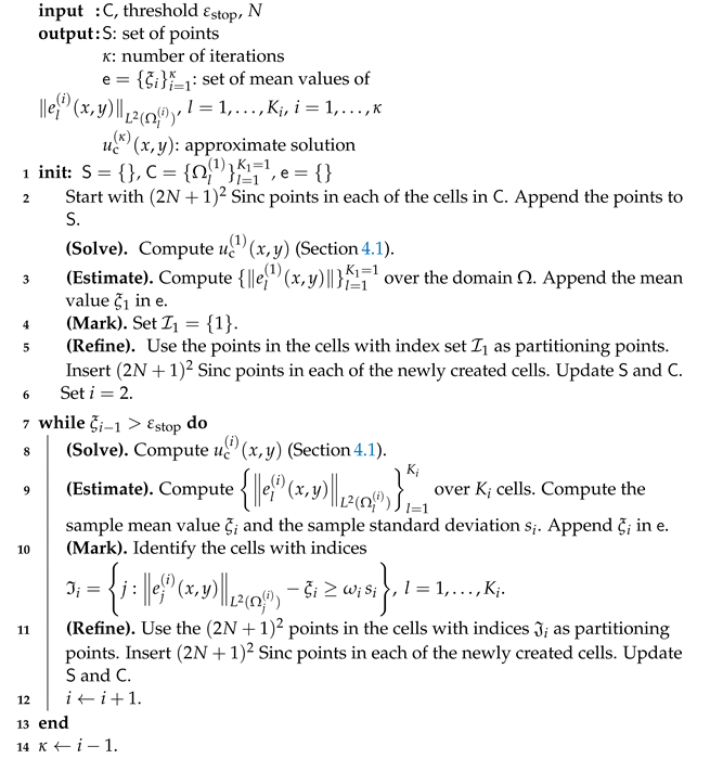
The adaptive Poly-Sinc-based LDG algorithm is outlined in Algorithm 1. The refinement strategy is performed as follows. For the ith iteration, we compute the set of L 2 norm values e l ( i ) ( x , y ) L 2 ( Ω l ( i ) ) l = 1 K i , where e l ( i ) ( x , y ) is defined in Section 4.1, over the K i cells, from which the sample mean ξ i = 1 K i l = 1 K i e l ( i ) ( x , y ) L 2 ( Ω l ( i ) ) and the sample standard deviation [51]
s i = 1 K i 1 l = 1 K i e l ( i ) ( x , y ) L 2 ( Ω l ( i ) ) ξ i 2
are computed [52,53,54]. The symbol Ω l ( i ) denotes the lth cell in the ith iteration. The cells with the indices I i = j : e j ( i ) ( x , y ) L 2 ( Ω j ( i ) ) ξ i ω i s i are marked for refinement, where the test of normality ω i is defined as [36]
ω i = 1 K i l = 1 K i e l ( i ) ( x , y ) L 2 ( Ω l ( i ) ) ξ i s i .
Using Hölder’s inequality for sums with p = q = 2  ([55], §3.2.8), one can show that ω i K i 1 K i < 1 . We restrict this to second-order moments only. The points in the cells with the indices I i are used as partitioning points, and ( 2 N + 1 ) 2 Sinc points are inserted in the newly created cells, where 2 N + 1 is the number of Sinc points in the x axis or the y axis. The algorithm terminates when the stopping criterion is satisfied. The approximate solution u c ( i ) ( x , y ) , i = 1 , , κ , for the ith iteration is computed using Equation (14).
The L 2 norm of a two-dimensional function f ( x , y ) is computed as follows:
f ( x , y ) L 2 ( Ω ) 2 = Ω f 2 ( x , y ) d x d y 1 / 2 ,
where the definite integral is computed numerically using a Sinc quadrature [38]; in other words, we have
a b f ( x ) d x h Q k = N N 1 φ ( x k ) f ( x k ) ,
where h Q is the Sinc spacing used for the Sinc quadrature, { x k } k = N N [ a , b ] represents the quadrature points, which are also Sinc points, and φ ( x ) is the conformal mapping in Section 2.1.   
Algorithm 1: Adaptive Poly-Sinc-based LDG algorithm.
Axioms 12 00227 i001

4.3. Error Analysis

We state below the main theorem:
Theorem 1
(Estimate of the upper bound). Let u be analytic and bounded in Ω, and let u c ( i ) ( x , y ) be the Poly-Sinc-based local discontinuous Galerkin approximation in the ith iteration. Let m x and m y be the number of Sinc points in the x axis and y axis, respectively. Let Λ be the Lebesgue constant. Let c j , k , l ( i ) be the estimated coefficients and u j , k , l ( i ) be the exact values of u ( x , y ) at the Sinc points { ( x j , l ( i ) , y k , l ( i ) ) } with
j , k , l | c j , k , l ( i ) u j , k , l ( i ) | < δ , i = 1 , 2 , , κ .
Then, there exists a constant A, independent of the ith iteration, such that
max ( x , y ) Ω u ( x , y ) u c ( i ) ( x , y ) K i E i + δ Λ m x Λ m y ,
where E i = A ( 2 r ) m λ m ( i 1 ) ( b a ) m x + Λ m x ( d c ) m y , r > 1 , and 0 < λ < 1 .
Proof. 
The derivation follows that of [34,35]. The upper bound on the error estimate u ( x , y ) u c ( i ) ( x , y ) is
max ( x , y ) Ω u ( x , y ) u c ( i ) ( x , y ) = u ( x , y ) u c ( i ) ( x , y ) Ω = u ( x , y ) u c ( i ) ( x , y ) + u h ( i ) ( x , y ) u h ( i ) ( x , y ) Ω u ( x , y ) u h ( i ) ( x , y ) Ω + u h ( i ) ( x , y ) u c ( i ) ( x , y ) Ω K i E i + l = 1 K i u h ( i ) ( x , y ) u c ( i ) ( x , y ) Ω l ( i ) = K i E i + l = 1 K i j = 1 m x k = 1 m y ( c j , k , l ( i ) u j , k , l ( i ) ) j , l ( i ) ( x ) k , l ( i ) ( y ) Ω l ( i ) K i E i + l = 1 K i j = 1 m x k = 1 m y | c j , k , l ( i ) u j , k , l ( i ) | | j , l ( i ) ( x ) | | k , l ( i ) ( y ) | Ω l ( i ) K i E i + δ K i l = 1 K i j = 1 m x k = 1 m y | j , l ( i ) ( x ) | | k , l ( i ) ( y ) | Ω l ( i ) = K i E i + δ K i l = 1 K i j = 1 m x | j , l ( i ) ( x ) | k = 1 m y | k , l ( i ) ( y ) | Ω l ( i ) K i E i + δ K i l = 1 K i j = 1 m x | j , l ( i ) ( x ) | Ω x , l ( i ) Λ m x , l ( i ) k = 1 m y | k , l ( i ) ( y ) | Ω y , l ( i ) Λ m y , l ( i ) K i E i + δ K i K i Λ m x ( i ) Λ m y ( i ) = K i E i + δ K i K i Λ m x Λ m y = K i E i + δ Λ m x Λ m y ,
where Ω l ( i ) = Ω x , l ( i ) × Ω y , l ( i ) , Λ m = 1 π log ( m ) + 1.07618 is the Lebesgue constant for the Poly-Sinc approximation [9,39,56], m x = max l m x , l , m y = max l m y , l , Λ m x = max l Λ m x , l , Λ m y = max l Λ m y , l , and the multiplicative property [57] of the supremum norm was used (i.e., x y x y ). The iteration index i was dropped in Λ m x , l ( i ) and Λ m y , l ( i ) since the number of interpolation points m x or m y is independent of the ith iteration. On average, the term | c j , k , l ( i ) u j , k , l ( i ) | < δ n i = δ K i m x m y < δ K i , where n i = K i m x m y is the total number of interpolation points in the ith iteration. Next, we derive the upper bound E i , which follows the derivation of [37,39]. We start with the computational domain Ω . An upper bound on the error estimate u u h becomes
u ( x , y ) u h ( i ) ( x , y ) Ω = u ( x , y ) L 1 ( L 2 ( u ( i ) ) ) Ω = u ( x , y ) L 1 ( L 2 ( u ( i ) ) ) + L 1 ( u ( i ) ) L 1 ( u ( i ) ) Ω u ( x , y ) L 1 ( u ( i ) ) Ω + L 1 ( u ( i ) ) L 1 ( L 2 ( u ( i ) ) ) Ω .
The upper bound of the error u ( x , y ) L 1 ( u ( i ) ) is
u ( x , y ) L 1 ( u ( i ) ) Ω = max ( x , y ) Ω u ( x , y ) L 1 ( u ( i ) ) = max ( x , y ) Ω u ( x , y ) j = 1 m x u ( x j ( i ) , y ) j ( i ) ( x ) max x [ a , b ] u ( x , y * ) j = 1 m x u ( x j ( i ) , y * ) j ( i ) ( x ) l = 1 K i max x Ω x , l u ( x , y * ) j = 1 m x u ( x j , l ( i ) , y * ) j , l ( i ) ( x ) l = 1 K i A x , l ( i ) ( 2 r x , l ( i ) ) m x ( L ( Ω x , l ( i ) ) ) m x N x , l ( i ) exp ( γ l , x ( i ) ( N x , l ( i ) ) β l , x ( i ) ) A x ( 2 r x ) m x ( L ( Ω x ( i ) ) ) m x l = 1 K i 1 = K i A x ( 2 r x ) m x ( λ x ) m x ( i 1 ) ( b a ) m x
where Ω l = Ω x , l × Ω y , l , A x = max l , i A x , l ( i ) N x , l ( i ) exp ( γ l , x ( i ) ( N x , l ( i ) ) β l , x ( i ) ) , r x = min l , i r x , l ( i ) , L ( Ω x ( i ) ) = max l L ( Ω x , l ( i ) ) , L ( Ω x ( i ) ) = λ x i 1 ( b a ) [35], where L ( · ) denotes the length, and
y * = y : u ( x , y ) j = 1 m x u ( x j ( i ) , y ) j ( i ) ( x ) is maximum x [ a , b ] and i .
The upper bound of the error L 1 ( u ( i ) ) L 1 ( L 2 ( u ( i ) ) ) is
L 1 ( u ( i ) ) L 1 ( L 2 ( u ( i ) ) ) Ω = L 1 ( u ( i ) L 2 ( u ( i ) ) ) Ω = max ( x , y ) Ω j = 1 m x u ( x j ( i ) , y ) k = 1 m y u ( x j ( i ) , y k ( i ) ) k ( i ) ( y ) j ( i ) ( x ) max y [ c , d ] u ( x * , y ) k = 1 m y u ( x * , y k ( i ) ) k ( i ) ( y ) max x [ a , b ] j = 1 m x j ( i ) ( x ) Λ m x Λ m x l = 1 K i max y Ω y , l u ( x * , y ) k = 1 m y u ( x * , y k , l ( i ) ) k , l ( i ) ( y ) Λ m x l = 1 K i A y , l ( i ) ( 2 r y , l ( i ) ) m y ( L ( Ω y , l ( i ) ) ) m y N y , l ( i ) exp ( γ l , y ( i ) ( N y , l ( i ) ) β l , y ( i ) ) Λ m x A y ( 2 r y ) m y ( L ( Ω y ( i ) ) ) m y l = 1 K i 1 = K i Λ m x A y ( 2 r y ) m y ( λ y ) m y ( i 1 ) ( d c ) m y ,
where A y = max l , i A y , l ( i ) N y , l ( i ) exp ( γ l , y ( i ) ( N y , l ( i ) ) β l , y ( i ) ) , r y = min l , i r y , l ( i ) , L ( Ω y ( i ) ) = max l L ( Ω y , l ( i ) ) , L ( Ω y ( i ) ) = λ y i 1 ( d c ) [35], and
x * = x : u ( x , y ) k = 1 m y u ( x , y k ( i ) ) k ( i ) ( y ) is maximum y [ c , d ] and i .
From the inequalities in Equations (20) and (21), the upper bound on the error estimate u u h becomes
u ( x , y ) u h ( i ) ( x , y ) Ω u ( x , y ) u h ( i ) ( x , y ) Ω = u ( x , y ) L 1 ( L 2 ( u ( i ) ) ) + L 1 ( u ( i ) ) L 1 ( u ( i ) ) Ω u ( x , y ) L 1 ( u ( i ) ) Ω + L 1 ( u ( i ) ) L 1 ( L 2 ( u ( i ) ) ) Ω K i A x ( 2 r x ) m x λ x m x ( i 1 ) ( b a ) m x + K i Λ m x A y ( 2 r y ) m y λ y m y ( i 1 ) ( d c ) m y K i A ( 2 r ) m λ m ( i 1 ) ( b a ) m x + Λ m x ( d c ) m y = K i E i ,
where m = min { m x , m y } , r = min { r x , r y } , λ = max { λ x , λ y } , A = max { A x , A y } , and
E i = A ( 2 r ) m λ m ( i 1 ) ( b a ) m x + Λ m x ( d c ) m x .
The inequality in Equation (19) becomes
max ( x , y ) Ω u ( x , y ) u c ( i ) ( x , y ) K i E i + δ Λ m x Λ m y .
We compute the mean value of the error estimate; in other words, we calculate
max ( x , y ) Ω 1 K i u ( x , y ) u c ( i ) ( x , y ) E i + δ K i Λ m x Λ m y .
For fitting purposes, we can rewrite the inequality in Equation (23) as
max ( x , y ) Ω 1 K i u ( x , y ) u c ( i ) ( x , y ) E i + δ K i Λ m x Λ m y = E i + δ ˜ Λ m x Λ m y ,
where δ ˜ = δ K i . We note that K i is increasing and K i is finite for a finite value of the iteration index i. The factor δ ˜ becomes small as K i , the number of cells in the ith iteration, becomes large.

4.4. Convergence Analysis of the Adaptive Algorithm

This section discusses the convergence of the adaptive algorithm. The convergence analysis for the one-dimensional case was shown in [35]. It suffices to show that the sequence { u c ( i ) ( x , y ) } is contractive and that it converges uniformly on Ω to u ( x , y ) .
Lemma 1
(Contraction mapping [58]). The sequence { u c ( i ) ( x , y ) } is contractive; in other words, there exists some constant 0 < C < 1 such that
u c ( i + 1 ) ( x , y ) u c ( i ) ( x , y ) Ω C u c ( i ) ( x , y ) u c ( i 1 ) ( x , y ) Ω .
Proof. 
Let K i + 1 , i , i 1 = K i + 1 K i K i 1 . Recalling the inequality in Equation (23), we have
1 K i + 1 , i , i 1 u c ( i + 1 ) ( x , y ) u c ( i ) ( x , y ) Ω = 1 K i + 1 , i , i 1 u c ( i + 1 ) ( x , y ) u c ( i ) ( x , y ) + u ( x , y ) u ( x , y ) Ω 1 K i + 1 , i , i 1 u ( x , y ) u c ( i + 1 ) ( x , y ) Ω + 1 K i + 1 , i , i 1 u ( x , y ) u c ( i ) ( x , y ) Ω < 1 K i + 1 u ( x , y ) u c ( i + 1 ) ( x , y ) Ω + 1 K i u ( x , y ) u c ( i ) ( x , y ) Ω E i + 1 + δ K i + 1 Λ m x Λ m y + E i + δ K i Λ m x Λ m y = E i + 1 + E i + δ Λ m x Λ m y 1 K i + 1 + 1 K i
Similarly, we have
1 K i + 1 , i , i 1 u c ( i ) ( x , y ) u c ( i 1 ) ( x , y ) Ω E i + E i 1 + δ Λ m x Λ m y 1 K i + 1 K i 1
We compare the ratio of the upper bounds in Equations (25) and (26); in other words, we have
θ = E i + 1 + E i + δ Λ m x Λ m y 1 K i + 1 + 1 K i E i + E i 1 + δ Λ m x Λ m y 1 K i + 1 K i 1 .
Since E i < E i 1 , i = 2 , , κ from Equation (22) and K i > K i 1 , i = 2 , , κ , one can directly verify that
E i + 1 + E i + δ Λ m x Λ m y 1 K i + 1 + 1 K i < E i + E i 1 + δ Λ m x Λ m y 1 K i + 1 K i 1 ,
In other words, θ < 1 . This implies that there is a constant C > 0 such that
1 K i + 1 , i , i 1 u c ( i + 1 ) ( x , y ) u c ( i ) ( x , y ) Ω C K i + 1 , i , i 1 u c ( i ) ( x , y ) u c ( i 1 ) ( x , y ) Ω .
Multiplying the inequality in Equation (26) by the constant C yields
C K i + 1 , i , i 1 u c ( i ) ( x , y ) u c ( i 1 ) ( x , y ) Ω C E i + E i 1 + δ Λ m x Λ m y 1 K i + 1 K i 1 .
From the inequalities in Equations (27) and (28), we have
1 K i + 1 , i , i 1 u c ( i + 1 ) ( x , y ) u c ( i ) ( x , y ) Ω C E i + E i 1 + δ Λ m x Λ m y 1 K i + 1 K i 1 .
The upper bound of the inequality in Equation (29) cannot be larger than that of Equation (25); in other words, we have
C E i + E i 1 + δ Λ m x Λ m y 1 K i + 1 K i 1 E i + 1 + E i + δ Λ m x Λ m y 1 K i + 1 + 1 K i .
This implies that C θ < 1 . Hence, there exists a constant 0 < C θ < 1 such that
1 K i + 1 , i , i 1 u c ( i + 1 ) ( x , y ) u c ( i ) ( x , y ) Ω C K i + 1 , i , i 1 u c ( i ) ( x , y ) u c ( i 1 ) ( x , y ) Ω .
Multiplying the inequality in Equation (30) by K i + 1 , i , i 1 , we obtain
u c ( i + 1 ) ( x , y ) u c ( i ) ( x , y ) Ω C u c ( i ) ( x , y ) u c ( i 1 ) ( x , y ) Ω .
Lemma 2
(Uniform convergence [37,58]). Let { u c ( i ) ( x , y ) } , i = 1 , 2 , be the sequence of bounded functions on Ω R 2 . If { u c ( i ) ( x , y ) } forms a Cauchy sequence on Ω, then
lim M sup j > M , k > M u c ( j ) ( x , y ) u c ( k ) ( x , y ) Ω = 0 ,
and the sequence { u c ( i ) ( x , y ) } converges uniformly on Ω to u ( x , y ) .
Proof. 
The derivation follows that of ([58], § 8.1.10). Since the sequence { u c ( i ) ( x , y ) } is contractive by Lemma 1, then the sequence { u c ( i ) ( x , y ) } is a Cauchy sequence ([58], Theorem 3.5.8). Hence, there exists a natural number M such that if j , k > M , then sup j > M , k > M u c ( j ) ( x , y ) u c ( k ) ( x , y ) Ω ϵ . Since ϵ is arbitrary, lim M sup j > M , k > M u c ( j ) ( x , y ) u c ( k ) ( x , y ) Ω = 0 . Hence, the sequence { u c ( i ) ( x , y ) } converges to a limit u ( x , y ) , ( x , y ) Ω . Let u : Ω R , where
u ( x , y ) : = lim i u c ( i ) ( x , y ) , ( x , y ) Ω .
It was shown in Theorem 1 that max ( x , y ) Ω 1 K i u ( x , y ) u c ( i ) ( x , y ) < E i + δ K i Λ m x Λ m y for ( x , y ) Ω . Since 0 < λ < 1 , then E i 0 as i . The term δ K i Λ m x Λ m y 0 as i since K i > 1 . We conclude that lim i u c ( i ) ( x , y ) = u ( x , y ) , ( x , y ) Ω , and the sequence { u c ( i ) ( x , y ) } converges uniformly on Ω to u ( x , y ) , which completes the proof. □
Lemmas (1) and (2) are used to prove the contraction mapping principle [37]. We consider the Banach space X = Ω [37]. While the supremum norm has a theoretical advantage, the L 2 norm will be used as discussed in [34]. Next, we will present some results for PDEs with Dirichlet boundary conditions and mixed Dirichlet-Neumann boundary conditions.

5. Numerical Examples

The results in this section were computed using Mathematica [59]. The Sinc spacing used for generating the Sinc points was h = h ( π 2 , 1 4 ) = π 1 2 N , and the Sinc spacing used for generating the quadrature points was h Q = π N . The stopping criterion ε stop = 10 4 . A precision of 200 digits was used. For all examples, we set the number of points per cell to be constant (i.e., m x m y = m 2 = ( 2 N + 1 ) 2 = 9 ). The traces were implemented as discussed in [60]. The number of quadrature points used in the Sinc quadrature (17) for a cell was ( 2 N + 1 ) 2 , where N = 20 . The number of quadrature points in a cell was increased to ( 2 1.5 N + 1 ) 2 if the width or the height of the cell was less than 10 3 .
Example 1.
Solution of two-dimensional Poisson equation [61] with Dirichlet boundary conditions:
Δ u = 2 π 2 sin ( π x ) sin ( π y ) ( x , y ) [ 0 , 1 ] 2 , u ( x , 0 ) = u ( x , 1 ) = 0 x [ 0 , 1 ] , u ( 0 , y ) = u ( 1 , y ) = 0 y [ 0 , 1 ] ,
whose exact solution is
u ( x , y ) = sin ( π x ) sin ( π y ) .
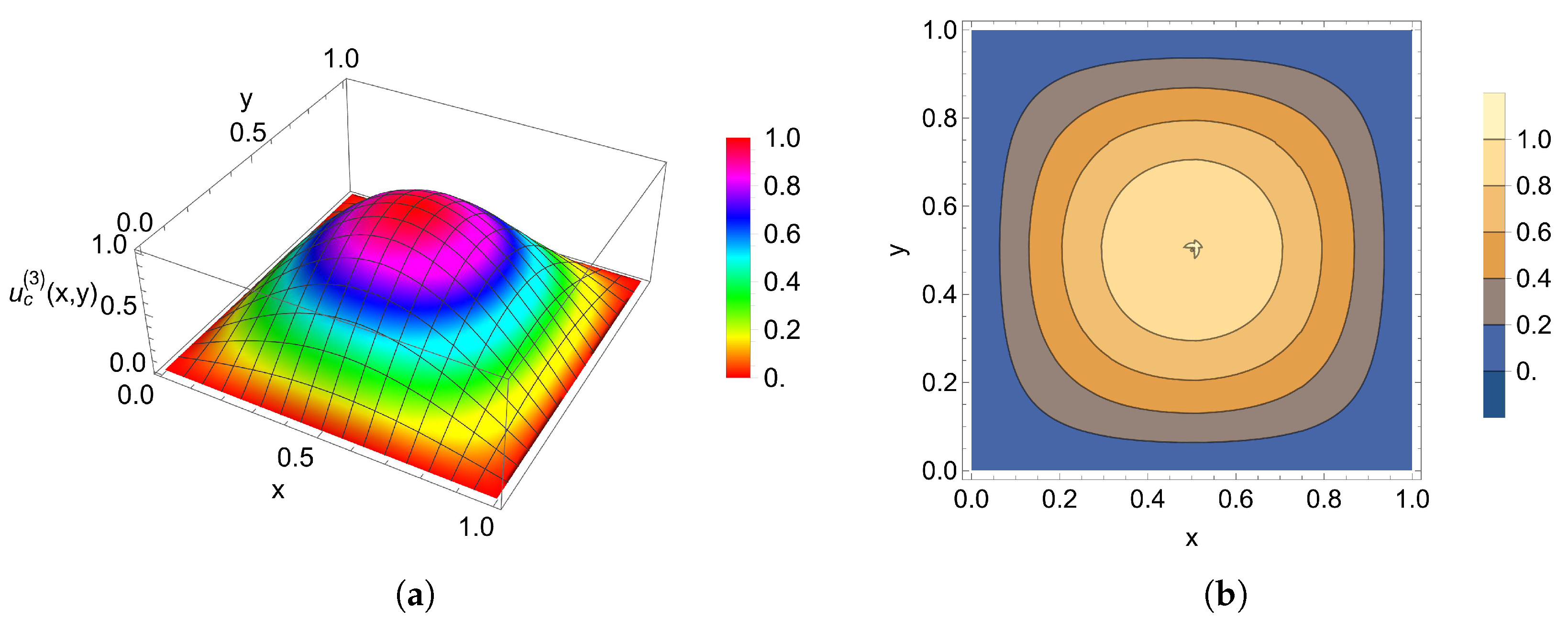
The algorithm terminates after κ = 3 iterations and the number of points | S | = 684 . Figure 2a shows the 3D plot of u c ( 3 ) ( x , y ) , and Figure 2b shows the contour plot of u c ( 3 ) ( x , y ) .
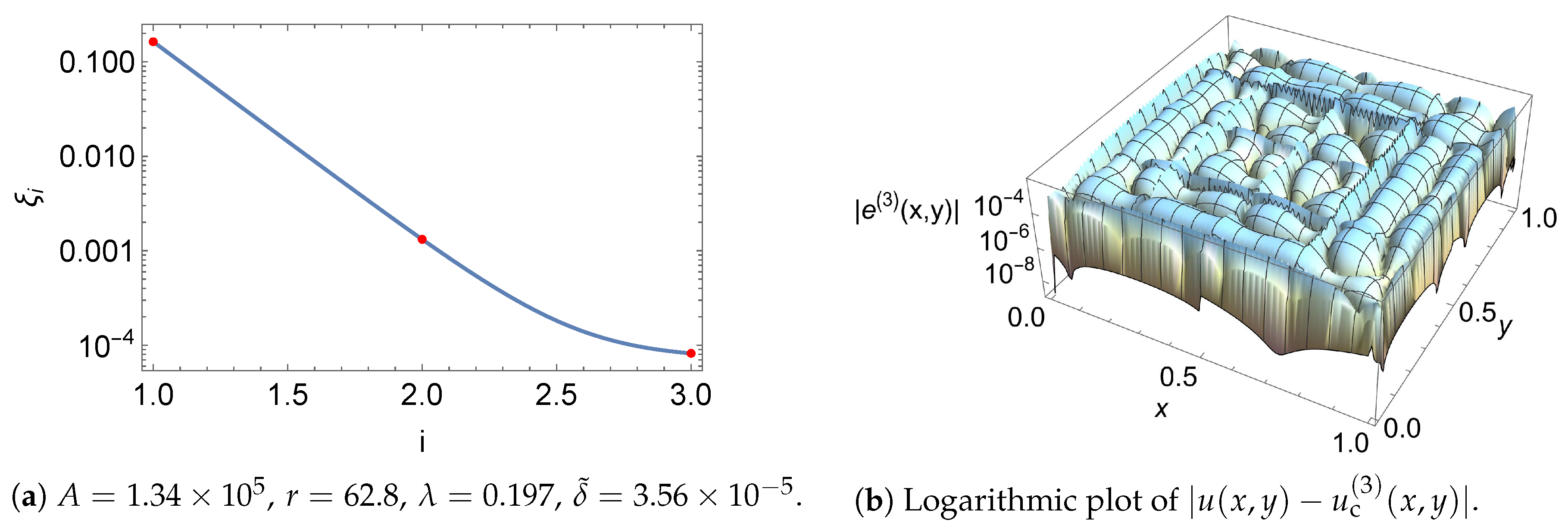
We perform least squares fitting of the logarithm of the set e to the logarithm of the upper bound of the inequality in Equation (24) as shown in Figure 3a. The dots represent the set e , and the solid line represents the least squares fitted model in Equation (24). The fitted model demonstrates an exponential decay in the mean value of e l ( i ) ( x , y ) , l = 1 , , K i , over the K i cells. The parameter δ ˜ , which results from the estimation of the coefficients of u c ( 3 ) ( x , y ) under the Poly-Sinc-based LDG method, is quite small. This indicates that our adaptive method can estimate the exact values of u ( x , y ) at the Sinc points up to a negligible error. Figure 3b shows the logarithmic plot of the absolute value of the local error e ( 3 ) ( x , y ) . The jumps in the local error plot result from the partitioning process of the Poly-Sinc-based LDG method. The jumps are almost negligible, as seen in Figure 2. The L 2 norm of the approximation error u ( x , y ) u c ( 3 ) ( x , y ) L 2 1.2 × 10 3 .
We tabulate the test of normality ω i as a function of the iteration index i , i = 2 , 3 , in Table 1. The test of normality ω i is less than one, as discussed in [34,35].
Example 2.
Consider the following Laplace equation [61] with Dirichlet boundary conditions:
Δ u = 0 ( x , y ) [ 1 , 1 ] 2 , u ( x , 1 ) = 0 x [ 1 , 1 ] , u ( 1 , y ) = u ( 1 , y ) = 0 y [ 1 , 1 ] , u ( x , 1 ) = sin ( π 2 x + 1 ) x [ 1 , 1 ] ,
whose exact solution is
u ( x , y ) = sinh ( π 2 y + 1 ) sin ( π 2 x + 1 ) sinh ( π ) .
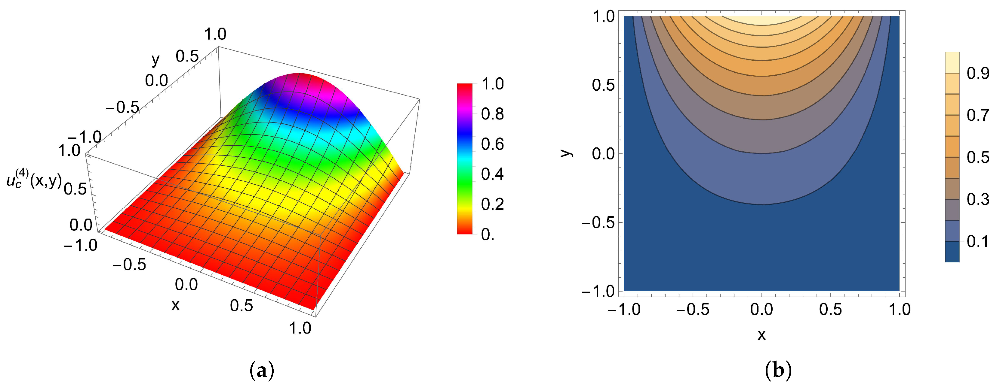
The algorithm terminates after κ = 4 iterations and the number of points | S | = 1494 . Figure 4a shows the 3D plot of u c ( 4 ) ( x , y ) , and Figure 4b shows the contour plot of u c ( 3 ) ( x , y ) .
We perform least squares fitting of the logarithm of the set e to the logarithm of the upper bound of the inequality in Equation (24) as shown in Figure 5a. The dots represent the set e , and the solid line represents the least squares fitted model in Equation (24). The fitted model demonstrates an exponential decay in the mean value of e l ( i ) ( x , y ) , l = 1 , , K i over the K i cells. The parameter δ ˜ , which results from the estimation of the coefficients of u c ( 4 ) ( x , y ) under the Poly-Sinc-based LDG method, is quite small. This indicates that our adaptive method can estimate the exact values of u ( x , y ) at the Sinc points up to a negligible error. Figure 5b shows the logarithmic plot of the absolute value of the local error e ( 4 ) ( x , y ) . The jumps in the local error plot result from the partitioning process of the Poly-Sinc-based LDG method. The jumps are almost negligible, as seen in Figure 4. The L 2 norm of the approximation error u ( x , y ) u c ( 4 ) ( x , y ) L 2 7.84 × 10 4 .
We tabulate the test of normality ω i as a function of the iteration index i , i = 2 , , 4 , in Table 2. The test of normality oscillates around the value ω i ¯ 0.67 .
Example 3.
Consider the following elliptic problem [43,62] with Dirichlet boundary conditions:
Δ u = f ( x , y ) in Ω , u ( x , y ) = 0 on Ω ,
where Ω = [ 1 , 4 ] × [ 0 , 1 ] and the exact solution is
u ( x , y ) = ( x + 1 ) ( x 4 ) ( 1 y 2 ) y 2 3.1596 .
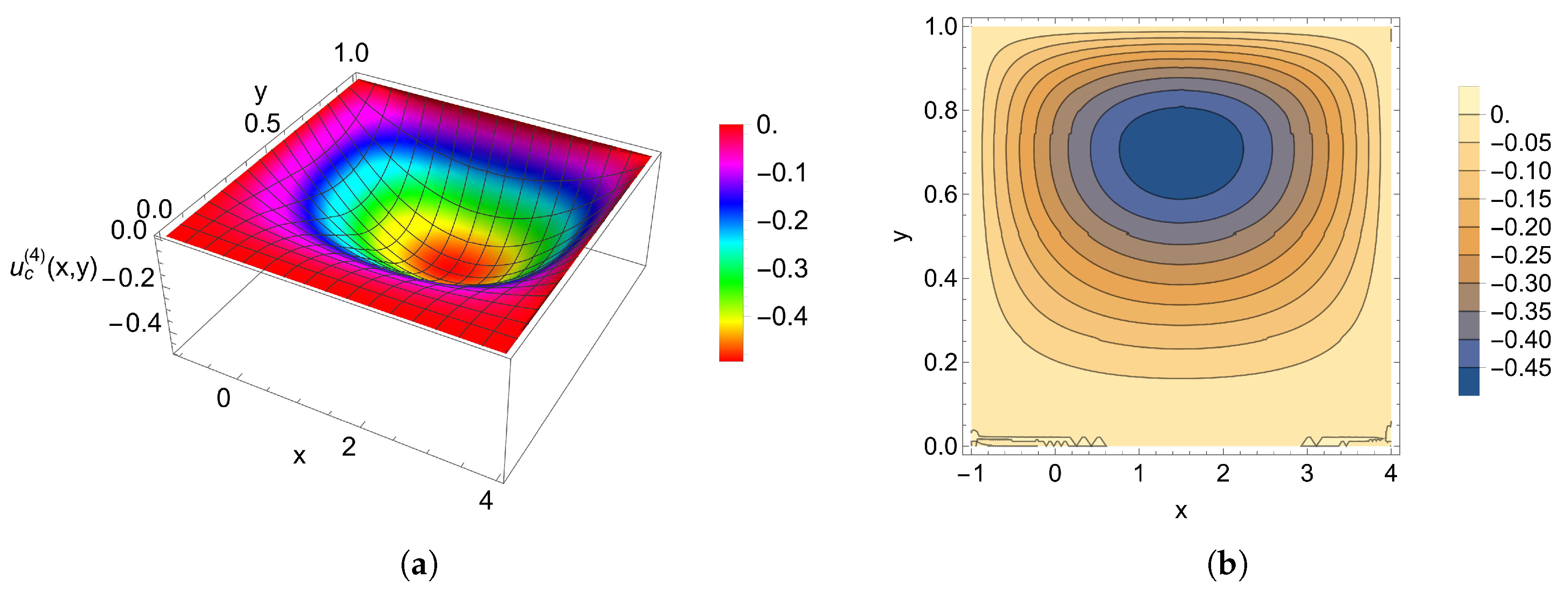
The algorithm terminates after κ = 4 iterations and the number of points | S | = 954 . Figure 6a shows the 3D plot of u c ( 4 ) ( x , y ) , and Figure 6b shows the contour plot of u c ( 4 ) ( x , y ) .
We perform least squares fitting of the logarithm of the set e to the logarithm of the upper bound of the inequality in Equation (24) as shown in Figure 7a. The dots represent the set e , and the solid line represents the least squares fitted model in Equation (24). The fitted model demonstrates an exponential decay in the mean value of e l ( i ) ( x , y ) , l = 1 , , K i , over the K i cells. The parameter δ ˜ , which results from the estimation of the coefficients of u c ( 4 ) ( x , y ) under the Poly-Sinc-based LDG method, is quite small. This indicates that our adaptive method can estimate the exact values of u ( x , y ) at the Sinc points up to a negligible error. Figure 7b shows the logarithmic plot of the absolute value of the local error e ( 4 ) ( x , y ) . The jumps in the local error plot result from the partitioning process of the Poly-Sinc-based LDG method. The jumps are almost negligible, as seen in Figure 6. The L 2 norm of the approximation error u ( x , y ) u c ( 4 ) ( x , y ) L 2 1.7 × 10 3 .
We tabulate the test of normality ω i , as a function of the iteration index i , i = 2 , , 4 , in Table 3. The test of normality oscillates around the value ω i ¯ 0.62 .
Example 4.
Consider the following Poisson problem [22] with mixed Dirichlet-Neumann boundary conditions:
Δ u = 8 π 2 sin ( 2 π ( x + y ) ) , ( x , y ) [ 0 , 1 ] 2 , u ( 0 , y ) = sin ( 2 π y ) , u ( x , 0 ) = sin ( 2 π y ) , x [ 0 , 1 ] , y [ 0 , 1 ] , u x ( 1 , y ) = 2 π cos ( 2 π y ) , u y ( x , 1 ) = 2 π cos ( 2 π x ) , x [ 0 , 1 ] , y [ 0 , 1 ] ,
whose exact solution is
u ( x , y ) = sin ( 2 π ( x + y ) ) .
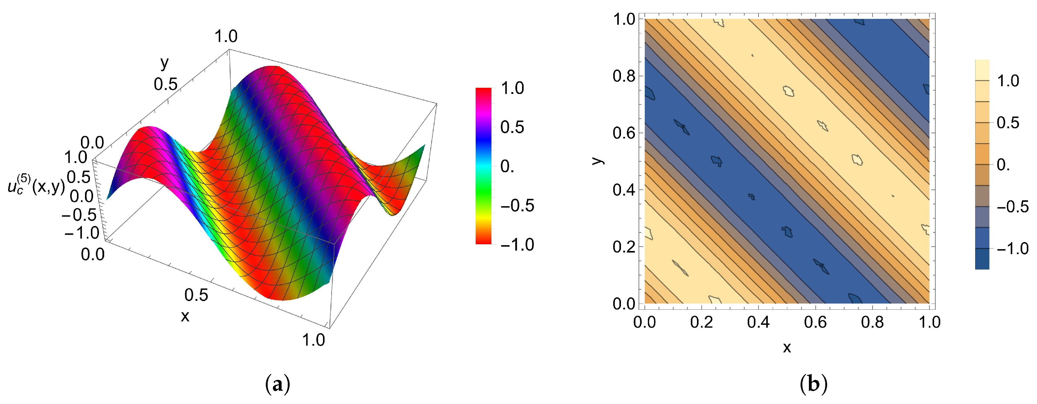
The algorithm terminates after κ = 5 iterations and the number of points | S | = 7839 . Figure 8a shows the 3D plot of u c ( 5 ) ( x , y ) , and Figure 8b shows the contour plot of u c ( 5 ) ( x , y ) .
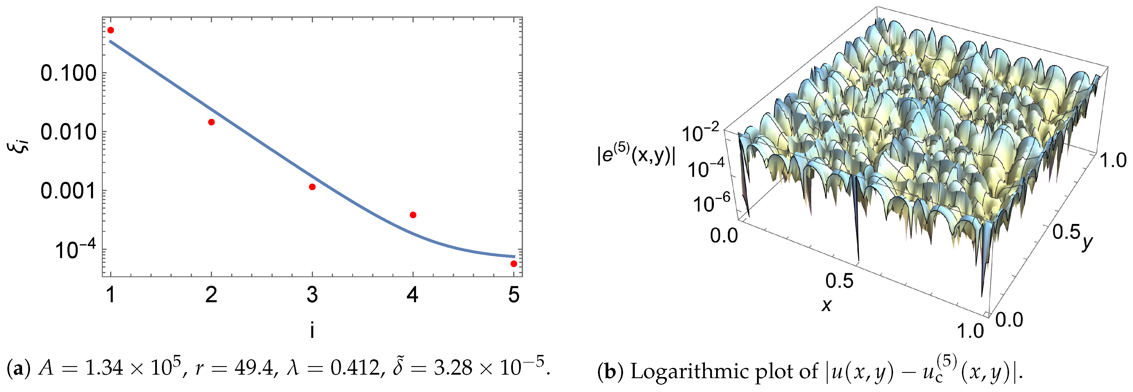
We perform least squares fitting of the logarithm of the set e to the logarithm of the upper bound of the inequality in Equation (24) as shown in Figure 9a. The dots represent the set e , and the solid line represents the least squares fitted model in Equation (24). The fitted model demonstrates an exponential decay in the mean value of e l ( i ) ( x , y ) , l = 1 , , K i , over the K i cells. The parameter δ ˜ , which results from the estimation of the coefficients of u c ( 5 ) ( x , y ) under the Poly-Sinc-based LDG method, is quite small. This indicates that our adaptive method can estimate the exact values of u ( x , y ) at the Sinc points up to a negligible error. Figure 9b shows the logarithmic plot of the absolute value of the local error e ( 5 ) ( x , y ) . The jumps in the local error plot result from the partitioning process of the Poly-Sinc-based LDG method. The jumps are almost negligible, as seen in Figure 8. The L 2 norm of the approximation error u ( x , y ) u c ( 5 ) ( x , y ) L 2 5.6 × 10 3 .
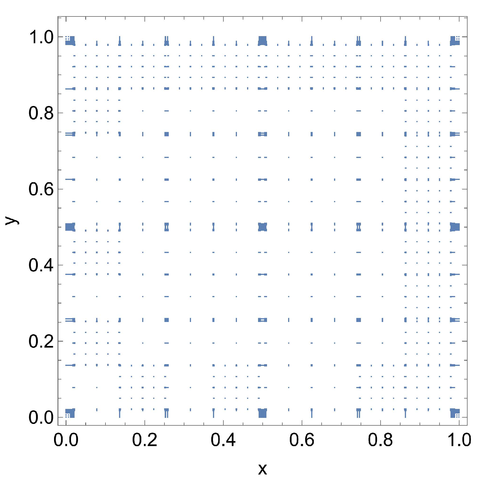
Figure 10 shows the distribution of the Sinc points for i = 5 . The plot shows a dense distribution of Sinc points near the boundaries as well as the center of the domain Ω.
We tabulate the test of normality ω i as a function of the iteration index i , i = 2 , , 5 , in Table 4. It can be observed that the test of normality ω i is decaying.

6. Conclusions

In this paper, we derived an a priori error estimate for the h-adaptive Poly-Sinc-based LDG algorithm and showed its exponential convergence in the number of iterations, provided that a good estimate of the exact solution u ( x , y ) at the Sinc points existed. The convergence of the adaptive algorithm was also shown. We used a statistical approach for refinement of the computational domain. We validated our adaptive method on elliptic PDEs with Dirichlet and mixed Neumann-Dirichlet boundary conditions. Our study demonstrates that better approximation can be obtained if the stopping criterion is less than 10 4 at the expense of more iterations.

Author Contributions

Conceptualization, G.B.; methodology, O.A.K.; software, O.A.K. and G.B.; validation, O.A.K. and G.B.; formal analysis, O.A.K.; investigation, O.A.K. and G.B.; resources, not applicable; data curation, not applicable; writing—original draft preparation, O.A.K.; writing—review and editing, G.B. and O.A.K.; visualization, O.A.K.; supervision, G.B.; project administration, G.B.; funding acquisition, not applicable. All authors have read and agreed to the published version of the manuscript.

Funding

This research received no external funding.

Institutional Review Board Statement

Not applicable.

Informed Consent Statement

Not applicable.

Data Availability Statement

Not applicable.

Acknowledgments

The authors thank the anonymous reviewers for their comments on an earlier draft of this paper.

Conflicts of Interest

The authors declare no conflict of interest.

References

  1. Reed, W.H.; Hill, T. Triangular Mesh Methods for the Neutron Transport Equation; Technical Report; Los Alamos Scientific Lab.: Los Alamos, NM, USA, 1973. [Google Scholar]
  2. Cockburn, B.; Karniadakis, G.E.; Shu, C.W. The Development of Discontinuous Galerkin Methods. In Discontinuous Galerkin Methods; Springer: Berlin/Heidelberg, Germany, 2000; pp. 3–50. [Google Scholar] [CrossRef] [Green Version]
  3. Cockburn, B.; Kanschat, G.; Perugia, I.; Schötzau, D. Superconvergence of the Local Discontinuous Galerkin Method for Elliptic Problems on Cartesian Grids. SIAM J. Numer. Anal. 2001, 39, 264–285. [Google Scholar] [CrossRef] [Green Version]
  4. Cockburn, B. Discontinuous Galerkin methods. ZAMM-J. Appl. Math. Mech. Angew. Math. Mech. Appl. Math. Mech. 2003, 83, 731–754. [Google Scholar] [CrossRef] [Green Version]
  5. Dolejší, V.; Feistauer, M. Discontinuous Galerkin Method: Analysis and Applications to Compressible Flow; Springer: Cham, Switzerland, 2015. [Google Scholar]
  6. Stenger, F. Polynomial function and derivative approximation of Sinc data. J. Complex 2009, 25, 292–302. [Google Scholar] [CrossRef] [Green Version]
  7. Stenger, F.; Youssef, M.; Niebsch, J. Improved approximation via use of transformations. In Multiscale Signal Analysis and Modeling; Springer: New York, NY, USA, 2013; pp. 25–49. [Google Scholar] [CrossRef]
  8. Stenger, F.; El-Sharkawy, H.A.M.; Baumann, G. The Lebesgue constant for Sinc approximations. In New Perspectives on Approximation and Sampling Theory: Festschrift in Honor of Paul Butzer’s 85th Birthday; Springer International Publishing: Cham, Switzerland, 2014; pp. 319–335. [Google Scholar] [CrossRef]
  9. Youssef, M.; El-Sharkawy, H.A.; Baumann, G. Lebesgue constant using Sinc points. Adv. Numer. Anal. 2016, 2016. [Google Scholar] [CrossRef] [Green Version]
  10. Lybeck, N.J.; Bowers, K.L. Domain decomposition via the Sinc-Galerkin method for second order differential equations. In Domain Decomposition Methods in Scientific and Engineering Computing, Proceedings of the 7th International Conference on Domain Decomposition, Pennsylvania, PA, USA, 27–30 October 1993; American Mathematical Society: Providence, RI, USA, 1994; pp. 271–276. [Google Scholar]
  11. Lybeck, N.J.; Bowers, K.L. Domain decomposition in conjunction with sinc methods for Poisson’s equation. Numer. Methods Partial. Differ. Equ. 1996, 12, 461–487. [Google Scholar] [CrossRef]
  12. Burda, P.; Novotný, J.; Šístek, J. Precise FEM solution of a corner singularity using an adjusted mesh. Int. J. Numer. Methods Fluids 2005, 47, 1285–1292. [Google Scholar] [CrossRef] [Green Version]
  13. Youssef, M.; Baumann, G. On bivariate Poly-Sinc collocation applied to patching domain decomposition. Appl. Math. Sci. 2017, 11, 209–226. [Google Scholar] [CrossRef]
  14. Frei, W. How to Identify and Resolve Singularities in the Model When Meshing. 2013. Available online: https://www.comsol.com/blogs/how-identify-resolve-singularities-model-meshing/ (accessed on 28 January 2023).
  15. Sönnerlind, H. Singularities in Finite Element Models: Dealing with Red Spots. 2015. Available online: https://www.comsol.com/blogs/singularities-in-finite-element-models-dealing-with-red-spots/ (accessed on 28 January 2023).
  16. Baumann, G.; Stenger, F. Fractional calculus and Sinc methods. Fract. Calc. Appl. Anal. 2011, 14, 568–622. [Google Scholar] [CrossRef]
  17. Cockburn, B.; Shu, C.W. The local discontinuous Galerkin method for time-dependent convection-diffusion systems. SIAM J. Numer. Anal. 1998, 35, 2440–2463. [Google Scholar] [CrossRef]
  18. Castillo, P.; Cockburn, B.; Perugia, I.; Schötzau, D. An A Priori Error Analysis of the Local Discontinuous Galerkin Method for Elliptic Problems. SIAM J. Numer. Anal. 2000, 38, 1676–1706. [Google Scholar] [CrossRef]
  19. Cockburn, B.; Kanschat, G.; Schötzau, D. The local discontinuous Galerkin method for linearized incompressible fluid flow: A review. Comput. Fluids 2005, 34, 491–506. [Google Scholar] [CrossRef]
  20. Yan, J.; Shu, C.W. Local discontinuous Galerkin methods for partial differential equations with higher order derivatives. J. Sci. Comput. 2002, 17, 27–47. [Google Scholar] [CrossRef]
  21. Castillo, P. A review of the Local Discontinuous Galerkin (LDG) method applied to elliptic problems. Appl. Numer. Math. 2006, 56, 1307–1313. [Google Scholar] [CrossRef]
  22. Baccouch, M. Optimal superconvergence and asymptotically exact a posteriori error estimator for the local discontinuous Galerkin method for linear elliptic problems on Cartesian grids. Appl. Numer. Math. 2021, 162, 201–224. [Google Scholar] [CrossRef]
  23. Cangiani, A.; Georgoulis, E.H.; Sabawi, Y.A. Adaptive discontinuous Galerkin methods for elliptic interface problems. Math. Comp. 2018, 87, 2675–2707. [Google Scholar] [CrossRef]
  24. Kompenhans, M.; Rubio, G.; Ferrer, E.; Valero, E. Adaptation strategies for high order discontinuous Galerkin methods based on Tau-estimation. J. Comput. Phys. 2016, 306, 216–236. [Google Scholar] [CrossRef] [Green Version]
  25. Kane, B.; Klöfkorn, R.; Dedner, A. Adaptive Discontinuous Galerkin Methods for Flow in Porous Media. In Proceedings of the Numerical Mathematics and Advanced Applications ENUMATH 2017, Voss, Norway, 25–29 September 2017; Radu, F.A., Kumar, K., Berre, I., Nordbotten, J.M., Pop, I.S., Eds.; Springer International Publishing: Cham, Switzerland, 2019; pp. 367–378. [Google Scholar] [CrossRef]
  26. Wang, F.; Ling, M.; Han, W.; Jing, F. Adaptive discontinuous Galerkin methods for solving an incompressible Stokes flow problem with slip boundary condition of frictional type. J. Comput. Appl. Math. 2020, 371, 112700. [Google Scholar] [CrossRef]
  27. Noventa, G.; Massa, F.; Rebay, S.; Bassi, F.; Ghidoni, A. Robustness and efficiency of an implicit time-adaptive discontinuous Galerkin solver for unsteady flows. Comput. Fluids 2020, 204, 104529. [Google Scholar] [CrossRef]
  28. Bassi, F.; Colombo, A.; Crivellini, A.; Fidkowski, K.J.; Franciolini, M.; Ghidoni, A.; Noventa, G. Entropy-Adjoint p-Adaptive Discontinuous Galerkin Method for the Under-Resolved Simulation of Turbulent Flows. AIAA J. 2020, 58, 3963–3977. [Google Scholar] [CrossRef]
  29. Bonev, B.; Hesthaven, J.S.; Giraldo, F.X.; Kopera, M.A. Discontinuous Galerkin scheme for the spherical shallow water equations with applications to tsunami modeling and prediction. J. Comput. Phys. 2018, 362, 425–448. [Google Scholar] [CrossRef] [Green Version]
  30. Beisiegel, N.; Vater, S.; Behrens, J.; Dias, F. An adaptive discontinuous Galerkin method for the simulation of hurricane storm surge. Ocean. Dyn. 2020, 70, 641–666. [Google Scholar] [CrossRef] [Green Version]
  31. Faghih-Naini, S.; Aizinger, V. p-adaptive discontinuous Galerkin method for the shallow water equations with a parameter-free error indicator. GEM-Int. J. Geomath. 2022, 13, 18. [Google Scholar] [CrossRef]
  32. Khalil, O.A.; Baumann, G. Discontinuous Galerkin methods using poly-sinc approximation. Math. Comput. Simul. 2021, 179, 96–110. [Google Scholar] [CrossRef]
  33. Khalil, O.A.; Baumann, G. Convergence rate estimation of poly-Sinc-based discontinuous Galerkin methods. Appl. Numer. Math. 2021, 165, 527–552. [Google Scholar] [CrossRef]
  34. Khalil, O.; El-Sharkawy, H.; Youssef, M.; Baumann, G. Adaptive piecewise Poly-Sinc methods for ordinary differential equations. Algorithms 2022, 15, 320. [Google Scholar] [CrossRef]
  35. Khalil, O.A.; El-Sharkawy, H.A.; Youssef, M.; Baumann, G. Adaptive piecewise Poly-Sinc methods for function approximation. Appl. Numer. Math. 2023, 186, 1–18. [Google Scholar] [CrossRef]
  36. Geary, R.C. The ratio of the mean deviation to the standard deviation as a test of normality. Biometrika 1935, 27, 310–332. [Google Scholar] [CrossRef]
  37. Stenger, F. Numerical Methods Based on Sinc and Analytic Functions; Springer Series in Computational Mathematics; Springer Science & Business Media: New York, NY, USA, 1993; Volume 20. [Google Scholar] [CrossRef]
  38. Stenger, F. Handbook of Sinc Numerical Methods; CRC Press: Boca Raton, FL, USA, 2011. [Google Scholar] [CrossRef]
  39. Youssef, M.; El-Sharkawy, H.A.; Baumann, G. Multivariate Lagrange interpolation at Sinc points: Error estimation and Lebesgue constant. J. Math. Res. 2016, 8, 4. [Google Scholar] [CrossRef] [Green Version]
  40. Baumann, G.; Stenger, F. Sinc-approximations of fractional operators: A computing approach. Mathematics 2015, 3, 444–480. [Google Scholar] [CrossRef] [Green Version]
  41. Stoer, J.; Bulirsch, R. Introduction to Numerical Analysis; Springer: New York, NY, USA, 2002. [Google Scholar] [CrossRef]
  42. Youssef, M.; Baumann, G. Collocation method to solve elliptic equations, Bivariate Poly-Sinc approximation. J. Progress. Res. Math. 2016, 7, 1079–1091. [Google Scholar]
  43. Youssef, M. Poly-Sinc Approximation Methods. Ph.D. Thesis, German University in Cairo, Cairo, Egypt, 2017. [Google Scholar]
  44. Rivière, B. Discontinuous Galerkin Methods for Solving Elliptic and Parabolic Equations: Theory and Implementation; SIAM: Philadelphia, PA, USA, 2008. [Google Scholar]
  45. Adjerid, S.; Chaabane, N. An improved superconvergence error estimate for the LDG method. Appl. Numer. Math. 2015, 98, 122–136. [Google Scholar] [CrossRef] [Green Version]
  46. Cormen, T.H.; Leiserson, C.E.; Rivest, R.L.; Stein, C. Introduction to Algorithms; MIT Press: Cambridge, MA, USA, 2009. [Google Scholar]
  47. Haasdonk, B.; Ohlberger, M. Reduced basis method for finite volume approximations of parametrized linear evolution equations. M2AN Math. Model. Numer. Anal. 2008, 42, 277–302. [Google Scholar] [CrossRef]
  48. Grepl, M.A. Model order reduction of parametrized nonlinear reaction–diffusion systems. Comput. Chem. Eng. 2012, 43, 33–44. [Google Scholar] [CrossRef]
  49. Sleeman, M.K.; Yano, M. Goal-oriented model reduction for parametrized time-dependent nonlinear partial differential equations. Comput. Methods Appl. Mech. Eng. 2022, 388, 114206. [Google Scholar] [CrossRef]
  50. Nochetto, R.H.; Siebert, K.G.; Veeser, A. Theory of adaptive finite element methods: An introduction. In Proceedings of the Multiscale, Nonlinear and Adaptive Approximation; DeVore, R., Kunoth, A., Eds.; Springer: Berlin/Heidelberg, Germany, 2009; pp. 409–542. [Google Scholar] [CrossRef]
  51. Walpole, R.E.; Myers, R.H.; Myers, S.L.; Ye, K. Probability and Statistics for Engineers and Scientists, 9th ed.; Pearson Education, Inc.: Boston, MA, USA, 2012. [Google Scholar]
  52. Carey, G.F.; Humphrey, D.L. Finite element mesh refinement algorithm using element residuals. In Proceedings of the Codes for Boundary-Value Problems in Ordinary Differential Equations; Childs, B., Scott, M., Daniel, J.W., Denman, E., Nelson, P., Eds.; Springer: Berlin/Heidelberg, Germany, 1979; pp. 243–249. [Google Scholar] [CrossRef]
  53. Carey, G.F. Adaptive refinement and nonlinear fluid problems. Comput. Methods Appl. Mech. Eng. 1979, 17–18, 541–560. [Google Scholar] [CrossRef]
  54. Carey, G.F.; Humphrey, D.L. Mesh refinement and iterative solution methods for finite element computations. Int. J. Numer. Methods Eng. 1981, 17, 1717–1734. [Google Scholar] [CrossRef]
  55. Abramowitz, M.; Stegun, I.A. Handbook of Mathematical Functions with Formulas, Graphs, and Mathematical Tables, 10th printing ed.; Dover Publications, Inc.: New York, NY, USA, 1972. [Google Scholar]
  56. Youssef, M.; Pulch, R. Poly-Sinc solution of stochastic elliptic differential equations. J. Sci. Comput. 2021, 87, 82. [Google Scholar] [CrossRef]
  57. Rudin, W. Functional Analysis; McGraw-Hill, Inc.: New York, NY, USA, 1973. [Google Scholar]
  58. Bartle, R.G.; Sherbert, D.R. Introduction to Real Analysis, 3rd ed.; John Wiley & Sons, Inc.: New York, NY, USA, 2000. [Google Scholar]
  59. Wolfram Research, Inc. Mathematica; Version 13.0; Wolfram Research, Inc.: Champaign, IL, USA, 2021. [Google Scholar]
  60. Arndt, D.; Bangerth, W.; Feder, M.; Fehling, M.; Gassmöller, R.; Heister, T.; Heltai, L.; Kronbichler, M.; Maier, M.; Munch, P.; et al. Reference Documentation for deal.II Version 9.4.1: The Step-12 Tutorial Program. 2023. Available online: https://www.dealii.org/current/doxygen/deal.II/step_12.html (accessed on 19 January 2023).
  61. Dell’Accio, F.; Di Tommaso, F.; Nouisser, O.; Siar, N. Solving Poisson equation with Dirichlet conditions through multinode Shepard operators. Comput. Math. Appl. 2021, 98, 254–260. [Google Scholar] [CrossRef]
  62. Lybeck, N.J. Sinc Domain Decomposition Methods for Elliptic Problems. Ph.D. Thesis, Montana State University, Bozeman, Montana, 1994. [Google Scholar]
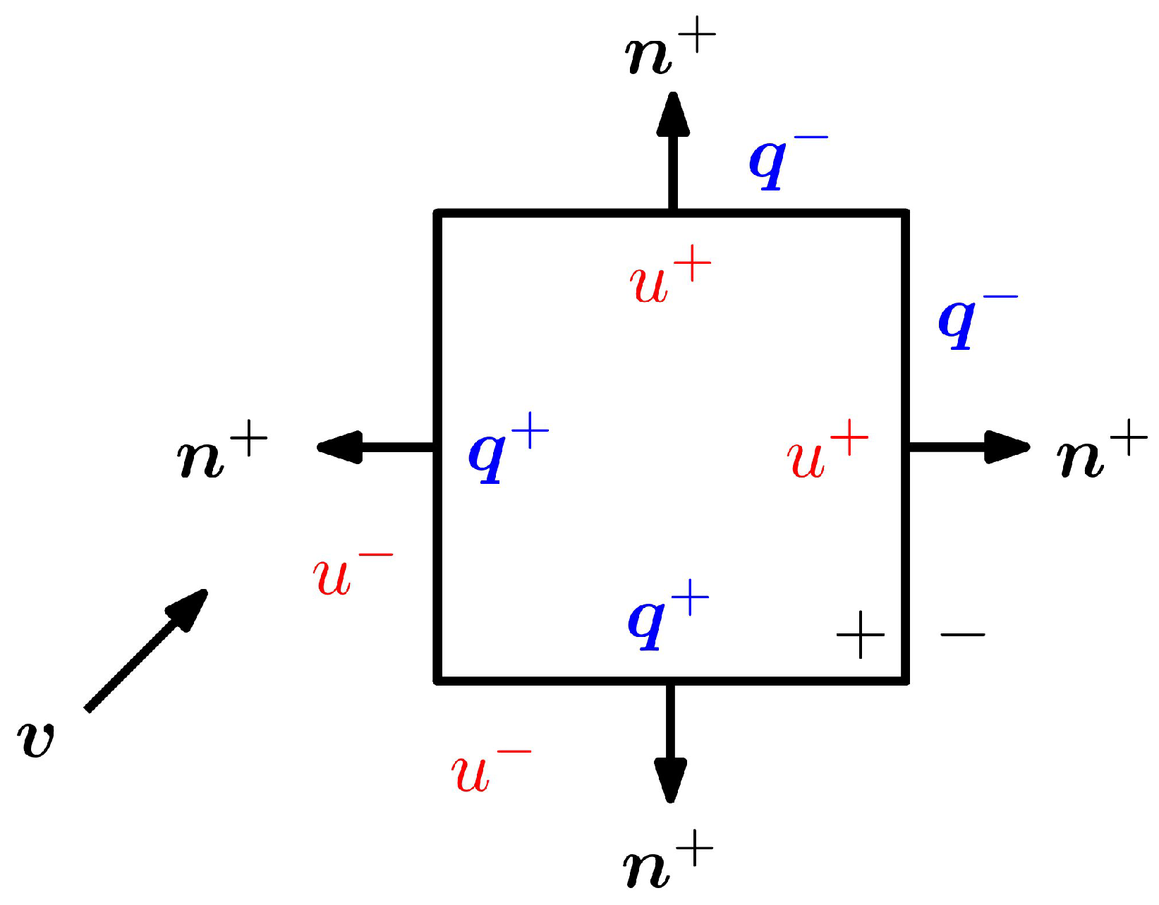
Figure 1. Illustration of u ^ is shown in red, and illustration of { { q } } C 12 q is shown in blue.
Axioms 12 00227 g001
Figure 2. A 3D plot and contour plot of u c ( 3 ) ( x , y ) for Example 1. (a) 3D plot of u c ( 3 ) ( x , y ) ; (b) Contour plot of u c ( 3 ) ( x , y ) .
Axioms 12 00227 g002
Figure 3. (a) Fitting the model in Equation (24) to the set e of Example 1. (b) Local error plot.
Axioms 12 00227 g003
Figure 4. A 3D plot and contour plot of u c ( 4 ) ( x , y ) for Example 2. (a) A 3D plot of u c ( 4 ) ( x , y ) ; (b) Contour plot of u c ( 4 ) ( x , y ) .
Axioms 12 00227 g004
Figure 5. (a) Fitting the model in Equation (24) to the set e of Example 2. (b) Local error plot.
Axioms 12 00227 g005
Figure 6. A 3D plot and contour plot of u c ( 4 ) ( x , y ) for Example 3. (a) 3D plot of u c ( 4 ) ( x , y ) ; (b) Contour plot of u c ( 4 ) ( x , y ) .
Axioms 12 00227 g006
Figure 7. (a) Fitting the model in Equation (24) to the set e of Example 3. (b) Local error plot.
Axioms 12 00227 g007
Figure 8. A 3D plot and contour plot of u c ( 5 ) ( x , y ) for Example 4. (a) 3D plot of u c ( 5 ) ( x , y ) ; (b) Contour plot of u c ( 5 ) ( x , y ) .
Axioms 12 00227 g008
Figure 9. (a) Fitting the model in Equation (24) to the set e of Example 4. (b) Plot of | u ( x , y ) u c ( 5 ) ( x , y ) | .
Axioms 12 00227 g009
Figure 10. Distribution of Sinc points for Example 4.
Axioms 12 00227 g010
Table 1. Test of normality ω i , i = 2 , 3 , for Example 1.
i ω i
2 0.8385
3 0.7718
Table 2. Test of normality ω i , i = 2 , , 4 , for Example 2.
i ω i
2 0.665
3 0.7206
4 0.6191
Table 3. Test of normality ω i , i = 2 , , 4 , for Example 3.
i ω i
2 0.7329
3 0.5189
4 0.5945
Table 4. Test of normality ω i , i = 2 , , 5 , for Example 4.
i ω i
2 0.8372
3 0.7744
4 0.7222
5 0.7002
Disclaimer/Publisher’s Note: The statements, opinions and data contained in all publications are solely those of the individual author(s) and contributor(s) and not of MDPI and/or the editor(s). MDPI and/or the editor(s) disclaim responsibility for any injury to people or property resulting from any ideas, methods, instructions or products referred to in the content.