Article

Estimations of Modified Lindley Parameters Using Progressive Type-II Censoring with Applications

1
Department of Mathematical Sciences, College of Science, Princess Nourah bint Abdulrahman University, P.O. Box 84428, Riyadh 11671, Saudi Arabia
2
Department of Statistics, Faculty of Science, King Abdulaziz University, Jeddah 21589, Saudi Arabia
3
Department of Statistics, Faculty of Commerce, Zagazig University, Zagazig 44519, Egypt
4
Faculty of Technology and Development, Zagazig University, Zagazig 44519, Egypt
*
Author to whom correspondence should be addressed.
Axioms 2023, 12(2), 171; https://doi.org/10.3390/axioms12020171
Submission received: 5 January 2023 / Revised: 29 January 2023 / Accepted: 4 February 2023 / Published: 7 February 2023

Abstract

:
This study addresses the estimation problems of the modified Lindley distribution using a progressive Type-II censoring plan. Using the maximum likelihood and maximum product of spacing and Bayesian estimation methods, the unknown parameter, reliability, and hazard rate functions are estimated. Employing the assumption of the gamma prior and a symmetric loss function, Bayes estimators are investigated when the observed data are obtained using the likelihood and product of spacing functions. Additionally, the approximate confidence intervals using both classical methods and the highest posterior density credible intervals are also discussed. To assess the different estimating strategies, a comprehensive simulation experiment that considers various sample sizes and censoring schemes is implemented. Finally, two actual data sets are examined to verify the utility of the modified Lindley distribution and the usefulness of the suggested estimators. The findings demonstrate that, in order to obtain the necessary estimators, the maximum product of the spacing method is preferred over the maximum likelihood method; whereas, when compared to the conventional techniques, the Bayesian approach using the likelihood and product of spacing functions provides more acceptable estimates.

1. Introduction

Chesneau et al. [1] introduced a novel one-parameter distribution derived from the Lindley distribution, which is called the modified Lindley (ML) distribution. Let X be a lifetime random variable of a test unit that follows the ML distribution, denoted by ML ( δ ) , then the probability density function (PDF), cumulative distribution function (CDF), reliability function (RF), and hazard rate function (HRF) of x > 0 , are given by
f ( x ; δ ) = δ 1 + δ e 2 δ x ( 1 + δ ) e δ x + 2 δ x 1 , δ > 0 ,
F ( x ; δ ) = 1 1 + δ x ( 1 + δ ) 1 e δ x e δ x ,
R ( x ; δ ) = 1 + δ x ( 1 + δ ) 1 e δ x e δ x
and
h ( x ; δ ) = δ + δ ( δ x 1 ) ( 1 + δ ) e δ x + δ x ,
respectively. Chesneau et al. [1] showed that the PDF in (1) can be unimodal or decreasing. Moreover, they demonstrated that the HRF is an unimodal function with an almost constant shape for large values of x. Their results of fitting the ML, Lindley, and exponential distributions to three real data sets revealed that the ML distribution is a powerful one-parameter rival. Veena and Lishamol [2] studied the different classical estimation methods of the ML distribution based on the complete sample data.
In a reliability analysis, the items of interest are typically lost or removed before failure. As a result, the obtained sample is known as a censored sample (or an incomplete sample). Preserving the functional experimental units for future use, shortening the duration of the test, and saving money are some major justifications for removing the experimental units. Various censoring plans, such as time and failure censoring, are available; however, they do not have the flexibility to permit items to be dropped at any moment other than the experiment’s termination point. As a result, the progressive Type-II censoring (PT-IIC) scheme, which is a more general censoring mechanism, is suggested. In practice, some items may be removed from the experiment for a more deep evaluation or saved to be used as test samples in further examinations. The following is a schematic representation of the PT-IIC sample: Assume that m units will stop working out of n distinct units that are run through a life test. Allow ( S 1 , S 2 , , S m ) to be fixed in advance such that when the first failure occurs at time X 1 : m : n , S 1 remaining units are arbitrarily removed from the experiment. When the experiment has its second failure time X 2 : m : n , S 2 remaining items are at random removed from the test, and so on. When the test experiences its m t h observed failure at time X m : m : n , all S m = n m i = 1 m 1 S i remaining surviving elements are removed from the test. If we assume that a continuous population with PDF f ( x ) and CDF F ( x ) , the likelihood function (LF) for a PT-IIC sample of size m can be written according to Balakrishnan [3], as follows
L ( δ ) = C i = 1 m f ( x i : m : n ) [ 1 F ( x i : m : n ) ] S i ,
where C is a parameter-free constant. In-depth research on the PT-IIC scheme has been conducted in the literature using a variety of lifetime distributions; see EL-Sagheer [4,5], Dey et al. [6], Chacko and Mohan [7], Nik et al. [8], Alotaibi et al. [9] and Maiti and Kayal [10]. One might read an outstanding review article by Balakrishnan [3] for additional information on the PT-IIC plan.
In recent years, it is common among authors to use the maximum product of the spacing (MPS) estimation method as a good alternative to the maximum likelihood method. Cheng and Amin [11] and Ranneby [12] independently proposed the MPS method and demonstrated that it retains the majority of the characteristics of the maximum likelihood method. In small sample cases for heavy-tailed or skewed distributions, Anatolyev and Kosenok [13] indicated that MPS estimators (MPSEs) are more effective than maximum likelihood estimators (MLEs). By choosing parameter values that maximize the product of the distances between the values of the CDF at consecutive ordering points, the MPSEs are founded. The product of the spacing (PS) function based on the PT-IIC sample, according to Ng et al. [14], has the following form
M ( δ ) = C i = 1 m + 1 [ F ( x i : m : n ) F ( x i 1 : m : n ) ] i = 1 m [ 1 F ( x i : m : n ) ] S i .
Many authors used the MPS method to investigate some lifetime distributions, see for example Mazucheli et al. [15], Rodrigues et al. [16], Almarashi [17] and Nassar et al. [18].
The novelty of this study comes from the fact that it is the first time to compare two classical and Bayesian (using LF and PS function) approaches of the ML distribution since its introduction. The importance of the PT-IIC scheme in improving the effectiveness of statistical inference when compared with Type-I and Type-II censoring schemes acts as the motivation for this study. Furthermore, two applications to actual data sets demonstrate the ML distribution’s capacity to fit various data types when compared with some competing lifetime distributions with one or two parameters. For the aim of estimation, the methods of maximum likelihood and MPS as well as the Bayesian approach are considered. In the Bayesian estimation, the posterior distribution of the unknown parameter is derived based on both the LF and PS function. The approximate confidence intervals (ACIs) and the highest posterior density (HPD) credible intervals are also considered. A simulation study and two applications to real data sets are taken into account to verify the offered approaches.
The rest of the paper is organized as follows: Section 2 displays the MLEs and MPSEs of the unknown parameters, RF and HRF, along with the corresponding ACIs. The Bayesian estimation using the Markov Chain Monte Carlo (MCMC) technique is considered in Section 3. The findings of the simulation study are shown in Section 4. In Section 5, two applications to actual data sets are examined. Lastly, Section 6 has provided conclusions.

2. Classical Estimation

In this part, the maximum likelihood and maximum product of the spacing estimation methods are used to obtain the point and interval estimators of the model parameter, as well as the RF and HRF. The interval estimators are produced using the asymptotic properties of the MLEs and MPSEs. The delta approach, on the other hand, is used to compute the approximate estimated variances of the RF and HRF estimators.

2.1. Maximum Lilekihood Estimation

Suppose that x = x i : m : n , i = , m are a PT-IIC sample of size m with progressive censoring scheme S i , i = 1 , , m collected from the ML population with PDF and CDF, as provided by (1) and (2), respectively. By neglecting the constant term, the likelihood function (LF) of the ML distribution in the presence of PT-IIC can be obtained from (1), (2) and (5), as shown below
L ( δ | x ) = δ δ ¯ m e δ i = 1 m ( 2 + S i ) x i i = 1 m δ ¯ e δ x i + 2 δ x i 1 1 + δ x i e δ x i δ ¯ S i ,
where δ ¯ = 1 + δ . The natural logarithm of (7) can be expressed as
log L ( δ | x ) = m [ log ( δ ) log ( δ ¯ ) ] δ i = 1 m ( 2 + S i ) x i + i = 1 m log δ ¯ e δ x i + 2 δ x i 1 + i = 1 m S i log 1 + δ x i e δ x i δ ¯ .
We obtain the following non-linear equation by differentiating the log-LF in (8) with regard to δ
d log L ( δ | x ) d δ = m δ δ ¯ i = 1 m ( 2 + S i ) x i + i = 1 m 2 x i + e δ x i [ 1 + ( 1 + δ ) x i ] δ ¯ e δ x i + 2 δ x i 1 i = 1 m S i x i e δ x i ( δ δ ¯ x i 1 ) δ ¯ [ 1 + δ ( 1 + x i e δ x i ) ] = 0 .
Because the normal equation in (9) has a complex form, the MLE of δ , represented by δ ^ , can be obtained numerically from (9) by applying the Newton Raphson procedure. Moreover, the MLEs of RF and HRF at a distinct time t can be obtained using the invariance property of the MLE. By changing the parameter δ in (3) and (4) by its MLE δ ^ , the MLEs of R ( t ) and h ( t ) are given, respectively, by
R ^ ( t ) = 1 + δ ^ t ( 1 + δ ^ ) 1 e δ ^ t e δ ^ t
and
h ^ ( t ) = δ ^ + δ ^ ( δ ^ t 1 ) ( 1 + δ ^ ) e δ ^ t + δ ^ t .
In addition to obtaining a point estimate for the unknown parameter, it is also useful to obtain a range of values that, with a certain degree of confidence, could contain the true parameter. In statistical inference, this process is known as interval estimation. Here, we suggest using the asymptotic normality of the MLE to build the ACI of δ . From the log-LF given by (8), we have
d 2 log L ( δ | x ) d δ 2 = m δ ¯ 2 m δ 2 i = 1 m 4 x i 2 + e δ x i ξ ( δ ¯ e δ x i + 2 δ x i 1 ) 2 i = 1 m S i ψ i δ ¯ [ 1 + δ ( 1 + x e δ x i ) ] 2 ,
where ξ = e δ x i e δ x i + 5 x i 2 + 6 x i + δ x i 2 ( 1 2 x i + 2 δ x i ) and ψ i = x i δ 2 ( 2 3 δ ¯ x i δ 2 x i ) + x i e δ x i ( 1 + 2 δ ) + 2 ( 1 + x i + δ + 2 δ x i ) δ x i 2 . For a sufficiently large PT-IIC sample, the asymptotic normality of the MLE δ ^ can be described as δ ^ N ( δ , I 1 ( δ ) ) , where I 1 ( δ ) is the variance-covariance matrix obtained through the Fisher information matrix. In practical problems, one may use the observed Fisher information to approximate the variance–covariance matrix. In this case, we have δ ^ N ( δ , I 1 ( δ ^ ) ) , where
I 1 ( δ ^ ) = d 2 log L ( δ | x ) d δ 2 δ = δ ^ 1 = V a r ^ ( δ ^ ) .
Accordingly, the ( 1 α ) % ACI of the parameter δ is [ δ ^ z α / 2 V a r ^ ( δ ^ ) , δ ^ + z α / 2 V a r ^ ( δ ^ ) ] , where z α / 2 is ( α / 2 ) t h upper percentile of the standard normal distribution. On the other hand, the asymptotic normality of the MLE can be used to construct the ACIs of R ( t ) and h ( t ) . To obtain such intervals, we consider utilizing the delta method to approximate the estimated variances of their estimators. Let Θ R = d R ( t ) d δ | δ = δ ^ and Θ h = d h ( t ) d δ | δ = δ ^ , where
d R ( t ) d δ = t e δ t 1 + e δ t ( 2 δ δ ¯ t 1 ) + δ ( 1 + δ ¯ ) δ ¯ 2
and
d h ( t ) d δ = 1 + 2 δ t 1 δ ¯ e δ t + δ t δ ( δ t 1 ) t + e δ t ( 1 + δ ˜ t ) ( δ ¯ e δ t + δ t ) 2 .
As a result, the required approximate estimated variances of R ^ ( t ) and h ^ ( t ) can be obtained, as shown below
V a r ^ ( R ^ ( t ) ) [ Θ R I 1 ( δ ^ ) Θ ´ R ] and V a r ^ ( h ^ ( t ) ) [ Θ h I 1 ( δ ^ ) Θ ´ h ] .
After obtaining the approximate variances, one can construct the ( 1 α ) % ACIs of RF and HRF as
R ^ ( t ) ± z α / 2 V a r ^ ( R ^ ( t ) ) and h ^ ( t ) ± z α / 2 V a r ^ ( h ^ ( t ) ) .

2.2. Maximum Product of Spacing Estimation

This is given a PT-IIC sample of size m, denoted by x = x i : m : n , i = , m , with a progressive censoring scheme S i , i = 1 , , m gathered from the ML population with PDF and CDF, as presented in (1) and (2), respectively. The PS function, ignoring the constant term, can be expressed in this case based on (1), (2) and (6), as follows
M ( δ | x ) = e δ i = 1 m S i x i δ ¯ m + 1 i = 1 m + 1 δ ¯ ( e δ x i 1 e δ x i ) + δ ( x i 1 e 2 δ x i 1 x i e 2 δ x i ) × i = 1 m 1 + δ x i e δ x i δ ¯ S i .
The natural logarithm of the PS function can be expressed as
log M ( δ | x ) = ( m + 1 ) log ( δ ¯ ) δ i = 1 m S i x i + i = 1 m + 1 log ( ϖ i ) + i = 1 m S i log 1 + δ x i e δ x i δ ¯ ,
where ϖ i = δ ¯ ( e δ x i 1 e δ x i ) + δ ( x i 1 e 2 δ x i 1 x i e 2 δ x i ) . Let δ ˜ denote the MPSE of the parameter δ . Then, δ ˜ can be acquired by solving the following nonlinear equation
d log M ( δ | x ) d δ = m + 1 δ ¯ i = 1 m S i x i i = 1 m + 1 ϑ i ϑ i 1 ϖ i i = 1 m S i x i e δ x i ( δ δ ¯ x i 1 ) δ ¯ [ 1 + δ ( 1 + x e δ x i ) ] = 0 ,
where ϑ i = ( 1 δ ¯ x i ) e δ x i x i ( 2 δ x i 1 ) e 2 δ x i . Since the nonlinear Equation (15) cannot be solved analytically, one can use a numerical technique such as the Newton-Raphson procedure to obtain the MPSE δ ˜ . According to Cheng and Traylor [19], the MPSE is consistent and shares the same asymptotic characteristics as the MLE. It exhibit the MLE’s invariance characteristic as well. Therefore, the MPSEs of R ( t ) and h ( t ) can be simply determined based on the invariance concept, respectively, as
R ˜ ( t ) = 1 + δ ˜ t ( 1 + δ ˜ ) 1 e δ ˜ t e δ ˜ t
and
h ˜ ( t ) = δ ˜ + δ ˜ ( δ ˜ t 1 ) ( 1 + δ ˜ ) e δ ˜ t + δ ˜ t .
Employing the asymptotic properties of the MPSE, the ACI of the parameter δ can be obtained. Practically, it is known that δ ˜ N ( δ , I 1 ( δ ˜ ) ) , where I 1 ( δ ˜ ) is the approximate variance-covariance matrix computed based on the observed Fisher information matrix, and expressed as follows
I 1 ( δ ˜ ) = d 2 log M ( δ | x ) d δ 2 δ = δ ˜ 1 = V a r ˜ ( δ ˜ ) ,
where
d 2 log M ( δ | x ) d δ 2 = m + 1 δ ¯ 2 i = 1 m + 1 η i η i 1 ϖ i + i = 1 m + 1 ( ϑ i ϑ i 1 ) 2 ϖ i 2 i = 1 m S i ψ i δ ¯ [ 1 + δ ( 1 + x e δ x i ) ] 2 ,
where η i = x i e δ x i ( δ x i 1 ) ( 4 x i e δ x i + 1 ) + x i 1 . Therefore, the ( 1 α ) % ACI of the parameter δ can be acquired as [ δ ˜ z α / 2 V a r ˜ ( δ ˜ ) , δ ˜ + z α / 2 V a r ˜ ( δ ˜ ) ] . The ACIs of the RF and HRF can be found by approximately estimating the variances of their estimators R ˜ ( t ) and h ˜ ( t ) using the delta approach, just as the MLE. The needed variances in this case are obtained as follows
V a r ˜ ( R ˜ ( t ) ) [ Θ R I 1 ( δ ˜ ) Θ ´ R ] and V a r ˜ ( h ˜ ( t ) ) [ Θ h I 1 ( δ ˜ ) Θ ´ h ] ,
where Θ R = d R ( t ) d δ | δ = δ ˜ and Θ h = d h ( t ) d δ | δ = δ ˜ , with d R ( t ) d δ and d h ( t ) d δ , as given by (11) and (12), respectively. Hence, the ACIs of the RF and HRF are as follows
R ˜ ( t ) ± z α / 2 V a r ˜ ( R ˜ ( t ) ) and h ˜ ( t ) ± z α / 2 V a r ˜ ( h ˜ ( t ) ) .

3. Bayesian Estimation

The conventional methods can occasionally even produce inaccurate and misleading results for experiments with small sample sizes or when censored data are present. In this case, the Bayesian approach could use more prior knowledge, such as historical data or knowledge in the statistical inferential process to obtain more accurate estimates. In this section, the Bayesian estimation of the parameter δ based on both the LF and PS function is considered. The squared error loss function is used to acquire the Bayes estimators of δ , R ( t ) , and h ( t ) , and the associated HPD credible intervals are also obtained. Under the assumption that the parameter δ has a gamma (G) prior distribution, the Bayes estimators are derived. The posterior distribution can be computed effectively thanks to this choice. Let δ G ( a , b ) , where a , b > 0 are the hyper-parameters. Then, the prior distribution of δ can be written as
π ( δ ) δ a 1 e b δ , δ > 0 .
In the next subsections, we use the LF and PS function to obtain the posterior distribution of the parameter δ and obtain the Bayes estimators as well as the HPD credible intervals of δ , R ( t ) , and h ( t ) .

3.1. Bayesian Estimation Using LF

The posterior density of δ is obtained as follows by combining the prior distribution in (16) with the LF given by (7)
g ( δ | x ) = δ m + a 1 A δ ¯ e δ [ i = 1 m ( 2 + S i ) x i + b ] i = 1 m δ ¯ e δ x i + 2 δ x i 1 1 + δ x i e δ x i δ ¯ S i ,
where
A = 0 δ m + a 1 δ ¯ e δ [ i = 1 m ( 2 + S i ) x i + b ] i = 1 m δ ¯ e δ x i + 2 δ x i 1 1 + δ x i e δ x i δ ¯ S i d δ .
The Bayes estimator for any function of the parameter δ , such as Ψ ( δ ) , can be determined by employing the squared loss function as
Ψ ^ B ( δ ) = 1 A 0 δ m + a δ ¯ e δ [ i = 1 m ( 2 + S i ) x i + b ] i = 1 m δ ¯ e δ x i + 2 δ x i 1 1 + δ x i e δ x i δ ¯ S i d δ .
It is obvious that an analytical method cannot be used to obtain the Bayes estimator in (18). In order to calculate the necessary estimators for δ , R ( t ) , and h ( t ) , as well as the accompanying HPD credible intervals, we suggest employing the MCMC procedure. We should first clearly define the conditional posterior distribution of δ in order to obtain these estimations. From (17), the conditional posterior distribution of δ can be expressed as follows
g * ( δ | x ) δ m + a 1 δ ¯ e δ [ i = 1 m ( 2 + S i ) x i + b ] i = 1 m δ ¯ e δ x i + 2 δ x i 1 1 + δ x i e δ x i δ ¯ S i .
The conditional distribution of δ cannot be reduced to any well-known density, as can be observed from (19). In order to produce samples from (19) with a normal proposal distribution, the Metropolis–Hastings (MH) technique is taken into consideration in this scenario. The steps below are used to create samples using the MH technique and obtain the Bayes estimates
Step 1.
Specify the initial value for δ , say δ ( 0 ) = δ ^ .
Step 2.
Set k = 1 .
Step 3.
Generate δ ( k ) from (19) with normal proposal distribution using the MH steps.
Step 4.
Taking a specific value for t, determine R ( k ) ( t ) and h ( k ) ( t ) as
R ( k ) ( t ) = 1 + δ k t ( 1 + δ k ) 1 e δ k t e δ k t
and
h ( j ) ( t ) = δ k + δ k ( δ k t 1 ) ( 1 + δ k ) e δ k t + δ k t .
Step 5.
Set k = k + 1 .
Step 6.
Replicate Steps 3 through 5, M times to obtain
δ ( 1 ) , R ( 1 ) ( t ) , h ( 1 ) ( t ) , , δ ( M ) , R ( M ) ( t ) , h ( M ) ( t ) , k = 1 , , M .
Step 7.
Compute the Bayes estimates, after removing M * samples as a burn-in period, as follows
δ ^ B = k = M * + 1 M δ ( k ) M M * , R ^ B ( t ) = k = M * + 1 M R ( k ) ( t ) M M * and h ^ B ( t ) = k = M * + 1 M h ( k ) ( t ) M M * .
Step 8.
To compute the HPD credible intervals, order δ ( k ) , R ( k ) ( t ) and h ( k ) ( t ) , k = M * + 1 , , M . Then, one can follow the method proposed by Chen and Shao [20] to obtain the required interval for the parameter δ , as follows
δ k * , δ k * + 1 α M M * ,
where k * = M * + 1 , M * + 2 , , M is chosen such that
δ k * + [ 1 α M M * ] δ k * = min 1 k α ( M M * ) ( δ ( k + [ 1 α M M * ] ) δ ( k ) ) .
The largest integer less than or equal to x is denoted by [ x ] . The same process can be applied to obtain the HPD credible intervals of R ( t ) and h ( t ) .

3.2. Bayesian Estimation Using PS Function

By combining the sample data given by the PF function as provided in (13), with the prior knowledge about the unknown parameter δ given by (16), the posterior distribution in this case can be presented as follows
q ( δ | x ) = δ a 1 e δ ( i = 1 m S i x i + b ) B δ ¯ m + 1 i = 1 m + 1 δ ¯ ( e δ x i 1 e δ x i ) + δ ( x i 1 e 2 δ x i 1 x i e 2 δ x i ) × i = 1 m 1 + δ x i e δ x i δ ¯ S i ,
where
B = 0 δ a 1 e δ ( i = 1 m S i x i + b ) δ ¯ m + 1 i = 1 m + 1 δ ¯ ( e δ x i 1 e δ x i ) + δ ( x i 1 e 2 δ x i 1 x i e 2 δ x i ) × i = 1 m 1 + δ x i e δ x i δ ¯ S i d δ .
It is clear that the Bayes estimator using the squared error loss function of the function Ψ ( δ ) cannot be calculated from (21) in a closed form, much like in the case of the Bayes estimator using the LF. As a result, we propose to use the MCMC technique to generate samples from (21) and compute the needed point and HPD credible estimates. To implement the MCMC method, we first derive the full conditional distribution of the parameter δ , as shown below
q * ( δ | x ) δ a 1 e δ ( i = 1 m S i x i + b ) δ ¯ m + 1 i = 1 m + 1 δ ¯ ( e δ x i 1 e δ x i ) + δ ( x i 1 e 2 δ x i 1 x i e 2 δ x i ) × i = 1 m 1 + δ x i e δ x i δ ¯ S i .
As expected, the conditional posterior distribution of δ cannot be analytically related to a well-known distribution, making direct sampling via conventional techniques impossible. Therefore, we employ the MH approach along with the normal proposal distribution to produce random samples from (22). The following are the steps involved in creating samples and computing the necessary estimates
Step 1.
Determine the initial value of δ by setting δ ( 0 ) = δ ˜ .
Step 2.
Put k = 1 .
Step 3.
Use MH steps to obtain δ ( k ) from (22) with normal proposal distribution.
Step 4.
At a mission time t, obtain R ( k ) ( t ) and h ( k ) ( t ) .
Step 5.
Put k = k + 1 .
Step 6.
Repeat Steps 3–5, M times to obtain δ ( k ) , R ( k ) ( t ) and h ( k ) ( t ) , k = 1 , , M .
Step 7.
Calculate the Bayes estimates as
δ ˜ B = k = M * + 1 M δ ( k ) M M * , R ˜ B ( t ) = k = M * + 1 M R ( k ) ( t ) M M * and h ˜ B ( t ) = k = M * + 1 M h ( k ) ( t ) M M * .
Step 8.
The same method mentioned in the previous part can be used to determine the HPD credible intervals.

4. Monte Carlo Simulations

Based on extensive Monte Carlo simulations, the performance of both point and interval estimators of δ , R ( t ) and h ( t ) derived by the proposed estimation methodologies in the proceeding sections is evaluated. To achieve this goal, we simulate 1000 PT-IIC samples using ML ( 0.5 ) and ML ( 1.5 ) based on various combinations of n(total test items), m(target sample size) and S (progressive censoring). Taking t = 0.25 , the actual values of ( R ( t ) , h ( t ) ) at δ = 0.5 and 1.5 are (0.9474,0.2602) and (0.7581,1.2664), respectively. Using n (=30,60,90), the choices of m are determined according to the failure percentages (FPs) m n (=40, 80)% of each n. Moreover, for each set of ( n , m ) , three progressive patterns S are considered, namely:
Scheme 1 : S = n m , 0 * ( m 1 ) ; Scheme 2 : S = 0 * m 2 1 , n m , 0 * m 2 ; Scheme 3 : S = 0 * ( m 1 ) , n m .
where 0 * ( m 1 ) , for example, stands that 0 is repeated ( m 1 ) times. Once the PT-IIC samples are collected, the ‘maxLik’ package (by Henningsen and Toomet [21]) in R 4.1.2 software is utilized to obtain the MLEs, MPSEs and 95% ACIs of δ , R ( t ) and h ( t ) . To calculate the Bayes point and interval estimates of δ , R ( t ) and h ( t ) , two informative priors of the gamma hyper-parameters ( a , b ) are adopted, namely: Prior-1: ( a , b ) = ( 2.5 , 5 ) and Prior-2: ( a , b ) = ( 5 , 10 ) (when δ = 0.5 ) as well as Prior-1: ( a , b ) = ( 7.5 , 5 ) and Prior-2: ( a , b ) = ( 15 , 10 ) (when δ = 1.5 ). Next, according to the MH algorithm via the ‘coda’ package (by Plummer et al. [22]), we simulate 12,000 MCMC samples from each unknown parameter and discard the first 2000 samples as the burn-in. Here, the hyper-parameter values are specified based on the prior mean and prior variance criteria. Then, from 10,000 MCMC samples, the Bayes estimates and 95% HPD credible interval estimates of δ , R ( t ) and h ( t ) are obtained. Comparison between the derived point estimates of δ , R ( t ) and h ( t ) (say φ ) derived from the frequentist (or Bayesian) is made based on two criteria called the root mean squared-errors (RMSEs) and mean relative absolute biases (MRABs), as
RMSE ( φ ˇ d ) = 1 K i = 1 K φ ˇ d ( i ) φ d 2 , d = 1 , 2 , 3 ,
and
MRAB ( φ ˇ d ) = 1 K i = 1 K 1 φ d φ ˇ d ( i ) φ d , d = 1 , 2 , 3 ,
respectively, where K is the number of generated sequence data, φ ˇ ( i ) is the calculated estimate of φ at the ith simulated sample, where φ 1 = δ , φ 2 = R ( t ) and φ 3 = h ( t ) . Comparison between the interval estimates of φ is also made using average confidence lengths (ACLs) and coverage percentages (CPs), respectively, as
ACL ( 1 α ) % ( φ k ) = 1 K i = 1 K U φ ˇ d ( i ) L φ ˇ d ( i ) , d = 1 , 2 , 3 ,
and
CP ( 1 α ) % ( φ k ) = 1 K i = 1 K 1 L φ ˇ d ( i ) ; U φ ˇ d ( i ) φ k , d = 1 , 2 , 3 ,
where ( L ( · ) , U ( · ) ) represents the (lower, upper) bound of the ( 1 α ) % interval estimate of φ d , and 1 ( · ) is the indicator function.
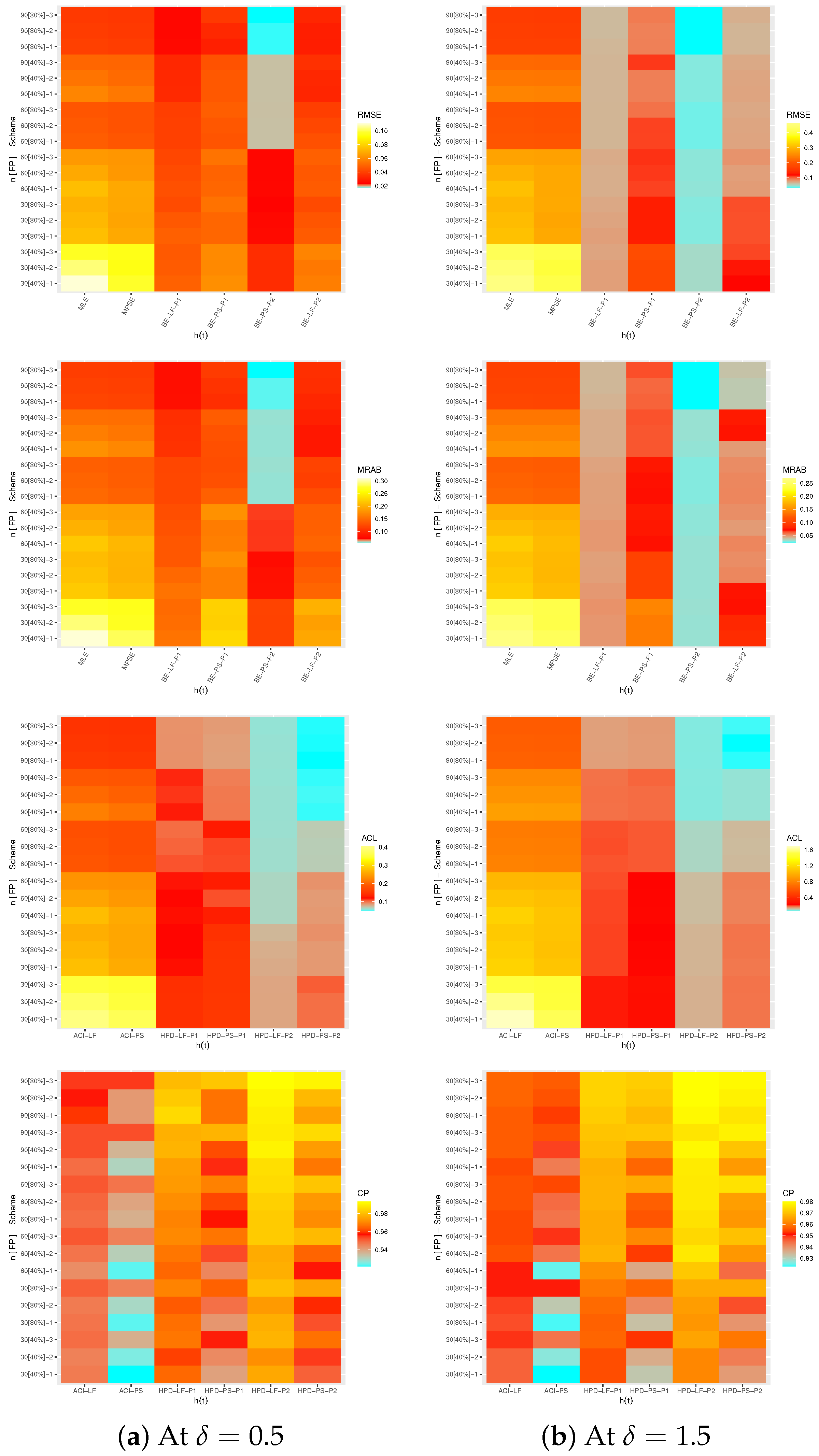
The results of δ , R ( t ) and h ( t ) are represented with heatmaps in Figure 1, Figure 2 and Figure 3, respectively. For each plot in Figure 1, Figure 2 and Figure 3, for Prior-1 (say P1) as an example, some notations of the estimation methods have been used such as (i) the Bayes estimate from the LF approach is mentioned as ‘‘BE-LF-P1’’; (ii) the Bayes estimate from the PS approach is noted as ‘‘BE-PS-P1’’; (iii) the HPD interval from the LF approach is described as ‘‘HPD-LF-P1’’; (iv) the HPD interval from the PS approach is mentioned as ‘‘HPD-PS-P1’’. Moreover, the ACI from LF and PS approaches are mentioned as ‘‘ACI-LF’’ and ‘‘ACI-PS’’, respectively. From Figure 1, Figure 2 and Figure 3, in terms of the lowest RMSE, MRAB and ACL values as well as the highest CP values, the following observations can be easily obtained:
  • All proposed estimates of δ , R ( t ) or h ( t ) behave well; this is the general comment.
  • When n(or m) grows, all estimates of δ , R ( t ) , and h ( t ) perform satisfactorily. When i = 1 m S i decreases, the same outcome is observed.
  • Due to the gamma prior, the MCMC estimates of δ , R ( t ) , and h ( t ) (from LF or PS) outperform the other estimates as expected. When comparing the HPD credible intervals to the ACIs, the same conclusion is reached.
  • It is obvious that the Bayes findings based on Prior 2 perform better than others for all unknown parameters, since the associated variance of Prior 2 is smaller than the associated variance of Prior 1.
  • All proposed estimates of δ , R ( t ) , and h ( t ) behave better utilizing scheme 3 than others when comparing the proposed censoring plans 1, 2 and 3.
  • Using the frequentist perspective, it can be observed that the proposed point estimates of δ , R ( t ) , and h ( t ) using the PS technique become even better than those derived from the LF approach in terms of the least RMSEs, MRABs, and ACLs. The ACI-PS interval estimates of δ , R ( t ) , and h ( t ) perform better than others in terms of ACLs criteria whereas the ACI-LF interval estimates of δ , R ( t ) , and h ( t ) perform better than others in terms of CPs criteria.
  • From the Bayesian perspective, it is clear that the proposed point estimates of δ , R ( t ) , and h ( t ) produced using the BE-LF approach are superior to those obtained using the BE-PS approach. It is also noted that the HPD-LF interval estimates δ , R ( t ) and h ( t ) perform better than others.
  • As δ increases, in most cases, the RMSEs, MRABs, and ACLs of δ , R ( t ) and h ( t ) increase while their CPs decrease.
  • To sum up, in order to estimate the unknown parameters of life δ , R ( t ) , and h ( t ) of the ML model using the PT-IIC data, we recommend using the PS approach (as a frequentist technique) and BE-LF (as a Bayesian method).

5. Real-Life Applications

In this section, two applications are explored to demonstrate the significance of the suggested estimation methods and to assess the ability for adapting the study objectives to actual situations.

5.1. Mechanical Equipment

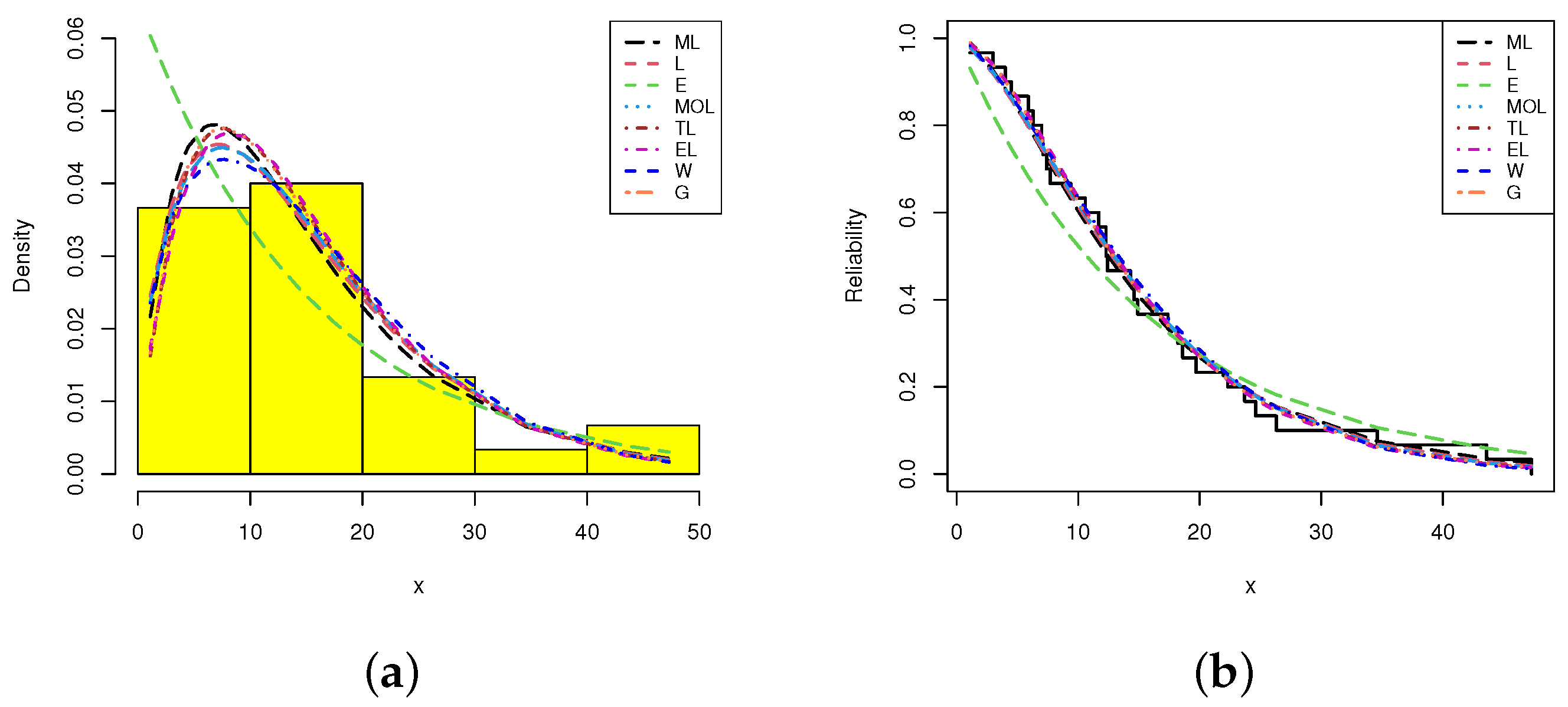
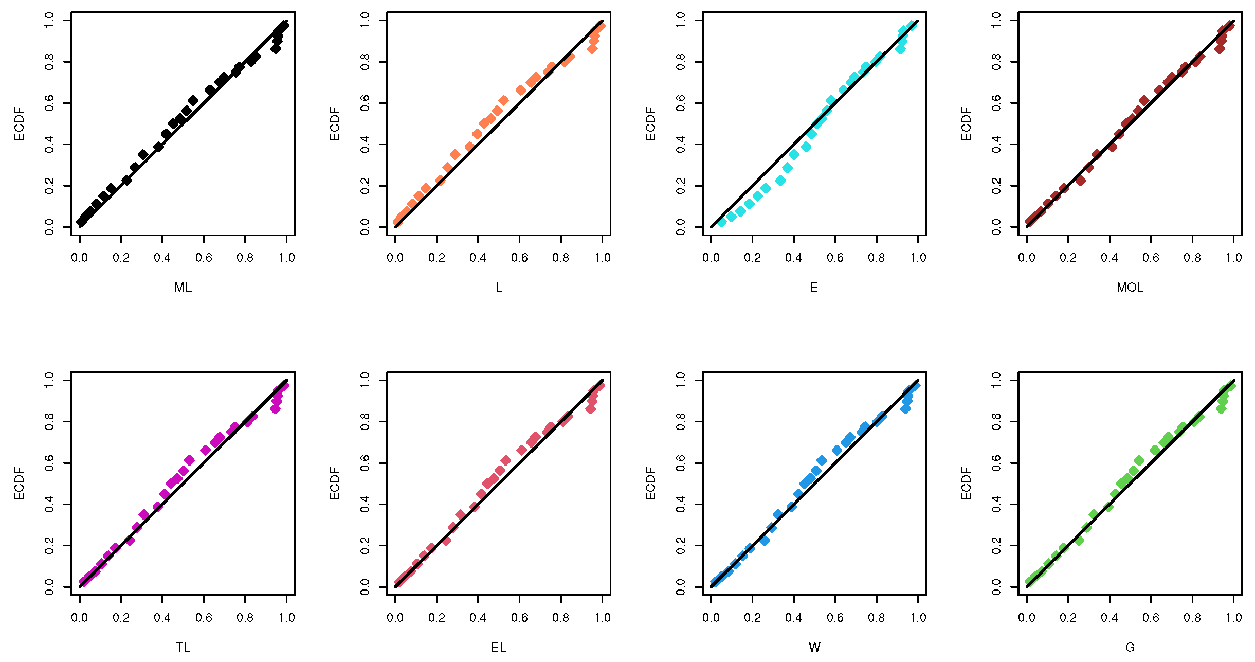
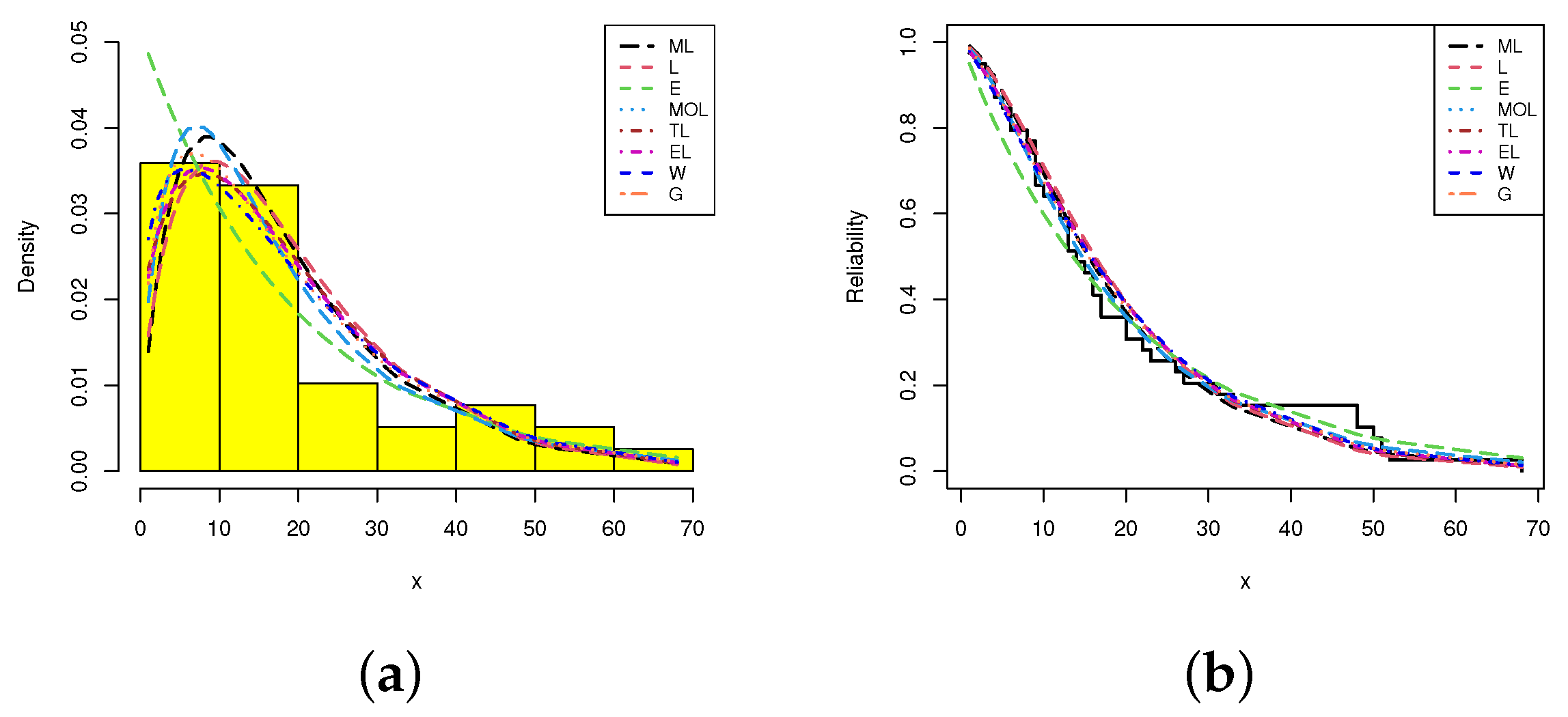
In this application, from Murthy et al. [23] and Elshahhat et al. [24], we shall use a real data set representing the time between failures of repairable mechanical equipment items; see Table 1. First, we compare the suitability of the ML distribution with some other models, namely, the Lindley (L ( δ ) ), exponential (E ( δ ) ), gamma (G ( β , δ ) ) and Weibull (W ( β , δ ) ), two-parameter Lindley (TL ( β , δ ) ) by Shanker and Mishra [25], exponentiated Lindley (EL ( β , δ ) ) by Nadarajah et al. [26] and Marshall-Olkin Lindley (MOL ( β , δ ) ) by Ghitany et al. [27] distributions. For computational convenience, each time point of the mechanical equipment data set is multiplied by ten. To judge the best distribution, several measures of fit are employed, namely: negative log-likelihood (NL), Akaike (A), consistent Akaike (CA), Bayesian (B), Hannan-Quinn (HQ) and the Kolmogorov–Smirnov (KS) statistic with its P-value. To establish this purpose, the MLE with its standard error (St.E) of each unknown parameter is calculated and presented in Table 2. It shows, in terms of the smallest of NL, A, CA, B, HQ, and KS values as well as the highest P-value, that the ML model has the best fit compared to others. Further, in Figure 4, quantile-quantile (QQ) plots of the ML and its competitive distributions are displayed. Furthermore, Figure 5a shows the histograms of mechanical equipment data and the fitted lines of the PDFs, and Figure 5b displays the fitted/empirical RFs of the ML and its competitive distributions. As expected, Figure 4 and Figure 5 support the same finding reported in Table 2.
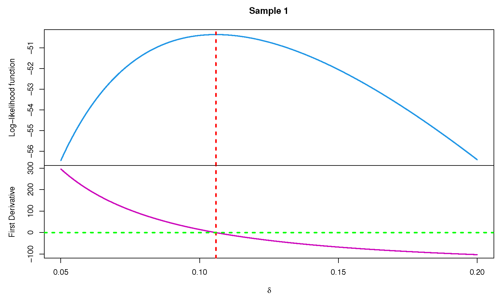
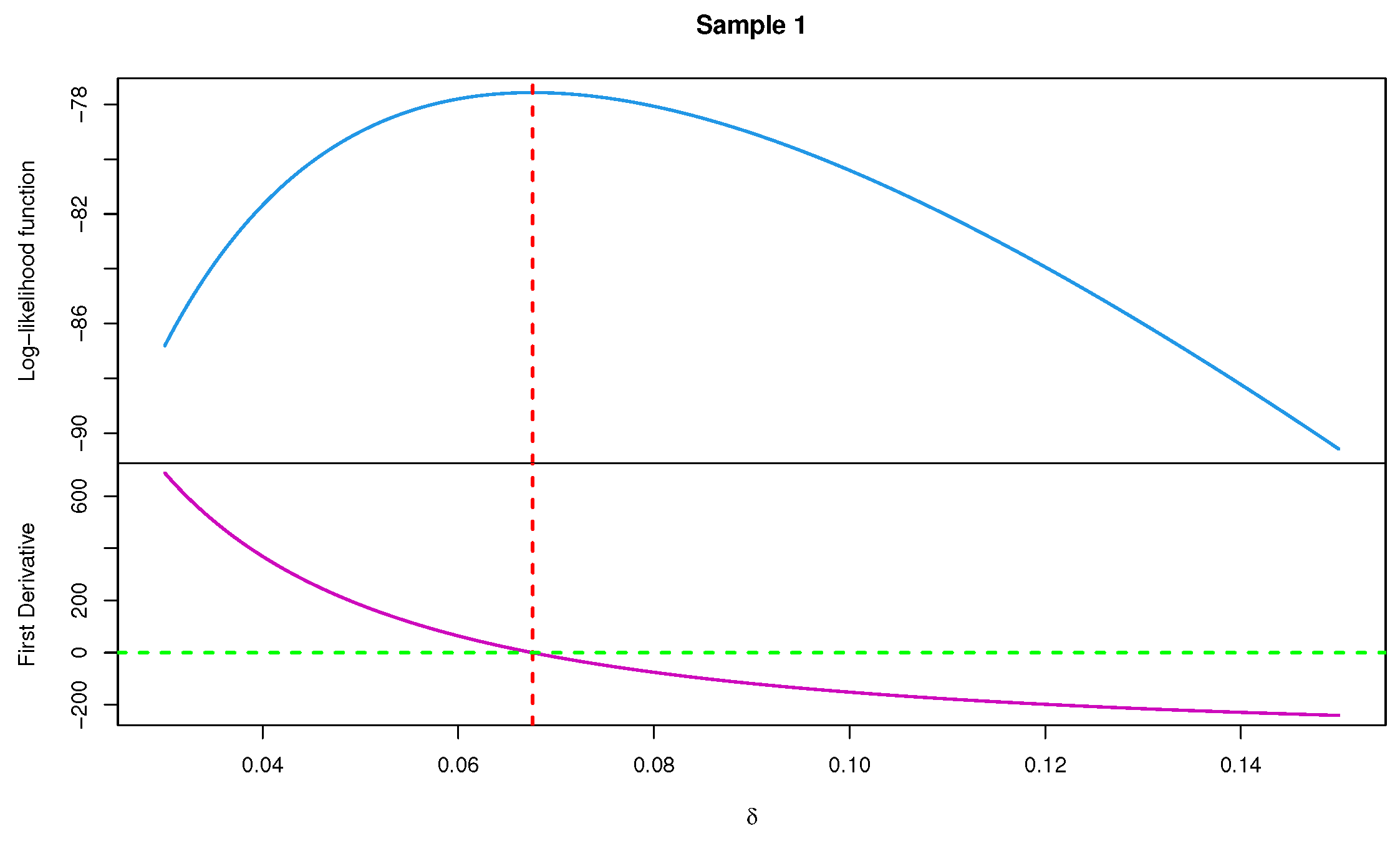
From the complete mechanical equipment data, by taking m = 15 , three artificial PT-IIC samples based on different progressive censoring schemes are generated and reported in Table 3. From Table 3, the frequentist estimates (including MLEs and MPSEs) and the Bayesian estimates (including BE-LF and BE-PS) with their St.Es of δ , R ( t ) and h ( t ) (at time t = 2 ) are obtained and reported in Table 4. Using the noninformative prior, each Bayes estimate is developed by running the MH algorithm 50,000 times and discarding the first 10,000 variates as a burn-in. Additionally, the 95% ACI/HPD credible interval estimates with their lengths are also calculated and provided in Table 4. To apply the proposed MCMC sampler, the calculated classical estimate of δ is used as an initial guess. It is clear, from Table 4, that the estimates of δ , R ( t ) and h ( t ) obtained by the MPSE (or BE-PS) procedure perform better compared to the MLEs’ (or BE-LF) procedure. A similar performance is also observed in the case of ACI-PS (or HPD-PS credible interval) estimates. Figure 6 displays the log-likelihood function and the associated first derivative of δ , given by (8) and (9), respectively, for sample 1 as an example. It demonstrates the existence and uniqueness of the MLE δ ^ .
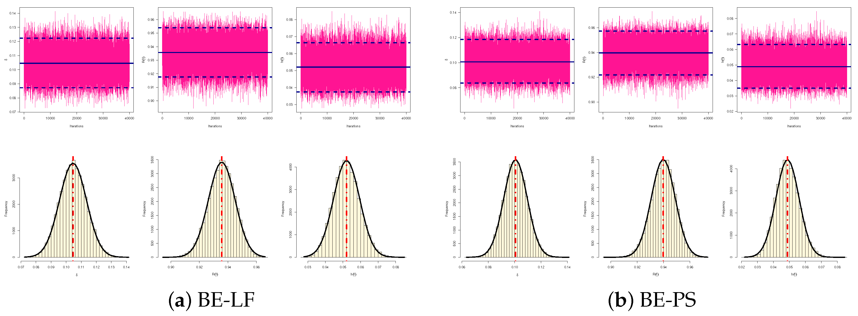
Moreover, several properties of the MCMC draws acquired by LF (or PS) of δ , R ( t ) and h ( t ) after the burn-in, namely: mean, mode, quartiles ( Q 1 , Q 2 , Q 3 ), standard deviation (St.D) and skewness are computed and provided in Table 5. From sample 1 (as an example), both MCMC trace and histogram plots with the fitted Gaussian kernel line of δ , R ( t ) and h ( t ) are displayed in Figure 7. In each trace plot, the sample mean and HPD credible interval bounds are represented by solid (—) and dashed (- - -) lines, respectively. Additionally, in each histogram plot, the sample mean is represented with a vertical-dotted (:) line. Figure 7 implies that the offered MCMC sampler converges satisfactorily and that the generated variates of δ , R ( t ) and h ( t ) are fairly-symmetric.

5.2. Motor Vehicle Deaths

In this application, the proposed estimators of the ML parameters are calculated based on real-life data obtained from the National Highway Traffic Safety Administration in the United States. This data set consists of the number of motor vehicle accident deaths (MVAD) for 39 counties in South Carolina for 2012; see Table 6. Recently, these data were reported and analyzed by Eghwerido et al. [28]. In Table 7, the calculated values of MLEs (with their St.Es), NL, A, CA, B, HQ, and KS (with its P-value) of the ML distribution and its competitive models are presented. This shows that the ML distribution provides the best overall fit compared to the others based on the criteria of NL, A, CA, B, and HQ while the G and MOL distributions also provide the best fit based on the KS(P-value) criterion. Moreover, using the complete MVAD data, Figure 8 supports the same numerical findings presented in Table 7. In addition, in Figure 9, the histograms of MVAD data with fitted PDFs as well as the fitted and empirical RFs are plotted. It is also evident that the ML distribution is the best model compared to its competitive models.
Presently, to discuss the derived point and interval estimators of δ , R ( t ) and h ( t ) , three different PT-IIC samples with size m = 20 are generated from the complete MVAD data and presented in Table 8. From Table 8, the MLEs, MPSEs, and Bayes estimates with their St.Es of δ , R ( t ) and h ( t ) (for t = 2 ) are computed and listed in Table 9. Moreover, two-sided 95% ACI/HPD credible interval estimates (developed by LF and PS approaches) with their lengths of δ , R ( t ) and h ( t ) are also obtained; see Table 9. It is observed, from Table 9, that the proposed point and interval estimates derived from the PS methodology performed better than those derived from the likelihood methodology in terms of the lowest St.Es and interval lengths. Figure 10 shows the log-likelihood function and the associated first derivative of δ , given by (8) and (9), respectively, for sample 1 as an example. It indicates that the MLE δ ^ exists and is unique. Using the generated sample 1, both trace and histogram plots of the MCMC variates of δ , R ( t ) and h ( t ) are provided in Figure 11. Various properties of the MCMC draws based on both LF and PS function are displayed in Table 10. It is evident that the MCMC sampler converges well and demonstrates that the simulated Markov chain variates of all unknown parameters are fairly symmetrical.
Finally, we may conclude that the proposed point/interval estimators generated by PS (or BE-PS) provide a reasonable demonstration of the ML model in the presence of a data set obtained from the PT-IIC plan based on both the mechanical equipment and motor vehicle data sets.

6. Concluding Remarks

In this study, using a progressive Type II censoring scheme, we took into account both Bayesian and non-Bayesian estimations of the parameter, reliability, and hazard functions of the modified Lindley distribution. In addition to obtaining the maximum likelihood and maximum product of the spacing point estimates, the approximate confidence intervals are also acquired. On the basis of the squared error loss function and the gamma prior assumption, the Bayesian estimations of the unknown parameters are proposed. It is noted that the Bayes estimators can be produced through numerical integration but cannot be obtained in explicit forms. We have therefore employed the Markov Chain Monte Carlo method to obtain the point estimates as well as the highest posterior density credible intervals. Through a simulation analysis for various sample sizes, various effective sample sizes, and various sampling plans, the performance of various approaches was examined. Additionally, two actual data sets were used to illustrate the validity of the proposed estimators. The numerical results demonstrated that the maximum product of the spacing method as a conventional approach is preferred to estimate the unknown parameter and reliability measures of the modified Lindley distribution. In contrast, when compared to the conventional approaches, the Bayesian estimation method employing both the likelihood or product of spacing functions is advised to acquire the point and interval estimates of the modified Lindley distribution.

Author Contributions

Methodology, M.N. and R.A.; Funding acquisition, R.A.; Software, A.E.; Supervision A.E.; Writing—original draft, R.A. and M.N.; Writing—review and editing, M.N. and A.E. All authors have read and agreed to the published version of the manuscript.

Funding

This research was funded by Princess Nourah bint Abdulrahman University Researchers Supporting Project number (PNURSP2023R50), Princess Nourah bint Abdulrahman University, Riyadh, Saudi Arabia.

Data Availability Statement

The authors confirm that the data supporting the findings of this study are available within the article.

Acknowledgments

The authors would like to express their thanks to the editor and the three referees for helpful comments and suggestions. Princess Nourah bint Abdulrahman University Researchers Supporting Project number (PNURSP2023R50), Princess Nourah bint Abdulrahman University, Riyadh, Saudi Arabia.

Conflicts of Interest

The authors declare no conflict of interest.

References

  1. Chesneau, C.; Tomy, L.; Gillariose, J. A new modified Lindley distribution with properties and applications. J. Stat. Manag. Syst. 2021, 24, 1383–1403. [Google Scholar] [CrossRef]
  2. Veena, G.; Lishamol, T. A comparative study of various estimation methods for modified Lindley distribution. Biom. Biostat. Int. J. 2022, 11, 79–81. [Google Scholar]
  3. Balakrishnan, N. Progressive Censoring Methodology: An Appraisal (with Discussion). TEST 2007, 16, 211–259. [Google Scholar] [CrossRef]
  4. EL-Sagheer, R.M. Estimation of parameters of Weibull–Gamma distribution based on progressively censored data. Stat. Pap. 2018, 59, 725–757. [Google Scholar] [CrossRef]
  5. El-Sagheer, R.M. Estimating the parameters of Kumaraswamy distribution using progressively censored data. J. Test. Eval. 2019, 47, 905–926. [Google Scholar] [CrossRef]
  6. Dey, S.; Nassar, M.; Maurya, R.K.; Tripathi, Y.M. Estimation and prediction of Marshall–Olkin extended exponential distribution under progressively type-II censored data. J. Stat. Comput. Simul. 2018, 88, 2287–2308. [Google Scholar] [CrossRef]
  7. Chacko, M.; Mohan, R. Statistical inference for Gompertz distribution based on progressive type-II censored data with binomial removals. Statistica 2018, 78, 251–272. [Google Scholar]
  8. Nik, A.S.; Asgharzadeh, A.; Raqab, M.Z. Estimation and prediction for a new Pareto-type distribution under progressive type-II censoring. Math. Comput. Simul. 2021, 190, 508–530. [Google Scholar]
  9. Alotaibi, R.; Nassar, M.; Rezk, H.; Elshahhat, A. Inferences and Engineering Applications of Alpha Power Weibull Distribution Using Progressive Type-II Censoring. Mathematics 2022, 10, 2901. [Google Scholar] [CrossRef]
  10. Maiti, K.; Kayal, S. Statistical Inferences to the Parameter and Reliability Characteristics of Gamma-mixed Rayleigh Distribution under Progressively Censored Data with Application. REVSTAT-Stat. J. 2022. Available online: https://revstat.ine.pt/index.php/REVSTAT/article/view/453. (accessed on 10 December 2022).
  11. Cheng, R.C.H.; Amin, N.A.K. Estimating parameters in continuous univariate distributions with a shifted origin. J. R. Stat. Soc. Ser. B Methodol. 1983, 45, 394–403. [Google Scholar] [CrossRef]
  12. Ranneby, B. The maximum spacing method. An estimation method related to the maximum likelihood method. Scand. J. Stat. 1984, 11, 93–112. [Google Scholar]
  13. Anatolyev, S.; Kosenok, G. An alternative to maximum likelihood based on spacings. Econom. Theory 2005, 21, 472–476. [Google Scholar] [CrossRef]
  14. Ng, H.K.T.; Luo, L.; Hu, Y.; Duan, F. Parameter estimation of three-parameter Weibull distribution based on progressively Type-II censored samples. J. Stat. Comput. Simul. 2012, 82, 1661–1678. [Google Scholar] [CrossRef]
  15. Mazucheli, J.; Ghitany, M.E.; Louzada, F. Comparisons of ten estimation methods for the parameters of Marshall–Olkin extended exponential distribution. Commun.-Stat.-Simul. Comput. 2017, 46, 5627–5645. [Google Scholar] [CrossRef]
  16. Rodrigues, G.C.; Louzada, F.; Ramos, P.L. Poisson–exponential distribution: Different methods of estimation. J. Appl. Stat. 2018, 45, 128–144. [Google Scholar] [CrossRef]
  17. Almarashi, A.M.; Algarni, A.; Nassar, M. On estimation procedures of stress-strength reliability for Weibull distribution with application. PLoS ONE 2020, 15, e0237997. [Google Scholar] [CrossRef]
  18. Nassar, M.; Dey, S.; Wang, L.; Elshahhat, A. Estimation of Lindley constant-stress model via product of spacing with Type-II censored accelerated life data. Commun.-Stat.-Simul. Comput. 2021. [Google Scholar] [CrossRef]
  19. Cheng, R.C.H.; Traylor, L. Non-regular maximum likelihood problems. J. R. Stat. Soc. Ser. B Methodol. 1995, 57, 3–24. [Google Scholar] [CrossRef]
  20. Chen, M.H.; Shao, Q.M. Monte Carlo estimation of Bayesian credible and HPD intervals. J. Comput. Graph. Stat. 1999, 8, 69–92. [Google Scholar]
  21. Henningsen, A.; Toomet, O. maxLik: A package for maximum likelihood estimation in R. Comput. Stat. 2011, 26, 443–458. [Google Scholar] [CrossRef]
  22. Plummer, M.; Best, N.; Cowles, K.; Vines, K. CODA: Convergence diagnosis and output analysis for MCMC. R News 2006, 6, 7–11. [Google Scholar]
  23. Murthy, D.N.P.; Xie, M.; Jiang, R. Weibull Models; Wiley Series in Probability and Statistics; Wiley: Hoboken, NJ, USA, 2004. [Google Scholar]
  24. Elshahhat, A.; Aljohani, H.M.; Afify, A.Z. Bayesian and Classical Inference under Type-II Censored Samples of the Extended Inverse Gompertz Distribution with Engineering Applications. Entropy 2021, 23, 1578. [Google Scholar] [CrossRef] [PubMed]
  25. Shanker, R.; Mishra, A. A two-parameter Lindley distribution. Stat. Transit. New Ser. 2013, 14, 45–56. [Google Scholar] [CrossRef]
  26. Nadarajah, S.; Bakouch, H.S.; Tahmasbi, R. A generalized Lindley distribution. Sankhya B 2011, 73, 331–359. [Google Scholar] [CrossRef]
  27. Ghitany, M.E.; Al-Mutairi, D.K.; Al-Awadhi, F.A.; Al-Burais, M.M. Marshall-Olkin extended Lindley distribution and its application. Int. J. Appl. Math. 2012, 25, 709–721. [Google Scholar]
  28. Eghwerido, J.T.; Ogbo, J.O.; Omotoye, A.E. The Marshall-Olkin Gompertz Distribution: Properties and Applications. Statistica 2021, 81, 183–215. [Google Scholar]
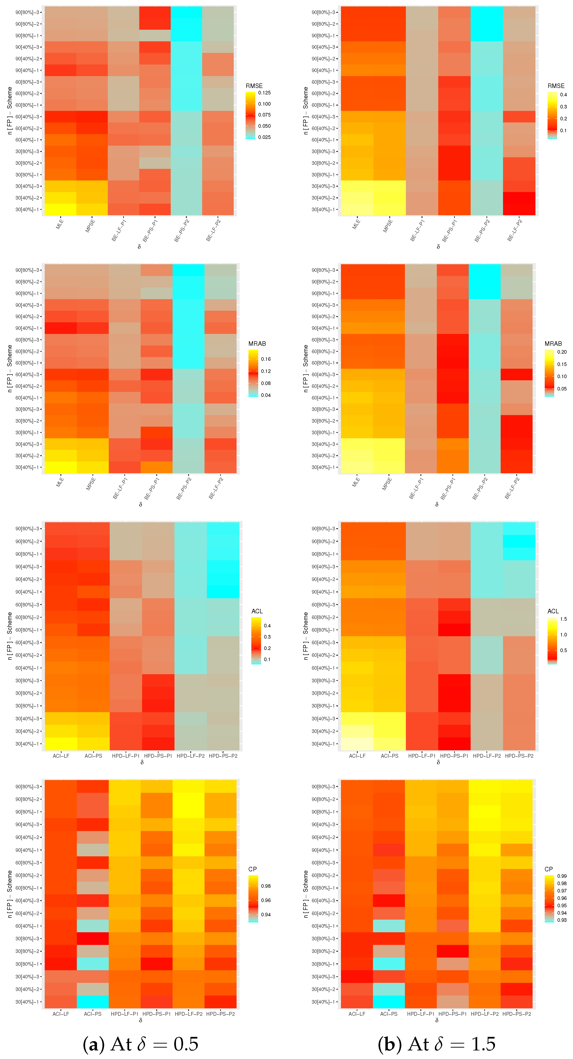
Figure 1. Heatmap plots for the simulation outputs of δ .
Axioms 12 00171 g001
Figure 2. Heatmap plots for the simulation outputs of R ( t ) .
Axioms 12 00171 g002
Figure 3. Heatmap plots for the simulation outputs of h ( t ) .
Axioms 12 00171 g003
Figure 4. The QQ plots of ML and its competitive models from mechanical equipment data.
Axioms 12 00171 g004
Figure 5. (a) Histograms/fitted PDFs; (b) empirical/fitted RF plots from mechanical equipment data.
Axioms 12 00171 g005
Figure 6. The log-likelihood function and the associated first derivative of δ from mechanical equipment data.
Axioms 12 00171 g006
Figure 7. Trace (top) and histograms (bottom) plots of δ , R ( t ) and h ( t ) from mechanical equipment data.
Axioms 12 00171 g007
Figure 8. The QQ plots of ML and its competitive models from MVAD data.
Axioms 12 00171 g008
Figure 9. (a) Histograms/fitted PDFs; (b) empirical/fitted RF plots from MVAD data.
Axioms 12 00171 g009
Figure 10. The log-likelihood function and the associated first derivative of δ from MVAD data.
Axioms 12 00171 g010
Figure 11. Trace (top) and histogram (bottom) plots of δ , R ( t ) and h ( t ) from MVAD data.
Axioms 12 00171 g011
Table 1. Times of repairable mechanical equipment.
1.13.04.04.55.96.37.07.17.47.7
9.410.611.712.312.312.414.314.614.917.4
18.218.619.722.323.724.626.334.643.647.3
Table 2. Summary of fit of ML and its competitive models from mechanical equipment data.
ModelMLE (St.E)NLACABHQKS (p-Value)
β δ
ML-0.0792 (0.0111)108.707219.770219.913221.171220.2190.0630 (0.999)
L-0.1225 (0.0159)108.942219.884220.027221.285220.3320.0688 (0.999)
E-0.0648 (0.0118)112.083226.166226.309227.567226.6140.1844 (0.259)
G1.9732 (0.4712)7.8105 (2.1200)108.711221.414221.859224.217222.3110.0669 (0.999)
W1.4633 (0.2029)17.099 (2.2539)108.988221.976222.420224.778222.8720.0749 (0.996)
TL0.0242 (1.4529)0.1294 (0.0206)108.771221.422221.867224.225222.3190.0692 (0.999)
EL1.1767 (0.3244)0.1330 (0.0243)108.885221.542221.986224.344222.4380.0751 (0.996)
MOL1.1345 (0.8926)0.1286 (0.0412)108.929221.859222.303224.661222.7550.0697 (0.999)
Table 3. Three PT-IIC samples from mechanical equipment data.
SampleSchemeCensored Data
1(15, 0 * 14)1.1, 3.0, 4.0, 4.5, 5.9, 7.0, 7.1, 7.7, 9.4, 12.3, 14.3, 17.4, 22.3, 24.6, 26.3
2 ( 0 * 6 , 5 * 3 , 0 * 6 ) 1.1, 3.0, 4.0, 4.5, 5.9, 6.3, 7.0, 7.4, 9.4, 10.6, 12.4, 14.6, 18.2, 22.3, 24.6
3 ( 0 * 14 , 15 ) 1.1, 3.0, 4.0, 4.5, 5.9, 6.3, 7.0, 7.1, 7.4, 7.7, 9.4, 10.6, 11.7, 12.3, 12.3
Table 4. Point and interval estimates of δ , R ( t ) , and h ( t ) from mechanical equipment data.
SamplePar.MLEBE-LFACI-LFHPD-LF
Est.St.EEst.St.ELowerUpperLengthLowerUpperLength
1 δ 0.10590.02090.10460.00910.06490.14680.08190.08720.12230.0351
R ( 2 ) 0.93460.02190.93570.00940.89160.97750.08590.91760.95400.0364
h ( 2 ) 0.05300.01740.05210.00750.01880.08710.06830.03750.06640.0290
2 δ 0.08080.01450.07970.00820.05240.10920.05680.06400.09590.0319
R ( 2 ) 0.95900.01300.95980.00730.93360.98450.05090.94560.97370.0281
h ( 2 ) 0.03350.01040.03290.00580.01310.05380.04070.02170.04420.0225
3 δ 0.07720.01350.07610.00810.05080.10360.05270.06080.09220.0314
R ( 2 ) 0.96220.01170.96290.00690.93930.98510.04580.94940.97630.0269
h ( 2 ) 0.03090.00940.03040.00560.01260.04930.03670.01960.04110.0215
MPSEBE-PSACI-PSHPD-PS
1 δ 0.10200.01990.10070.00900.06290.14100.07810.08380.11860.0348
R ( 2 ) 0.93860.02050.93970.00920.89850.97870.08020.92190.95730.0354
h ( 2 ) 0.04980.01630.04890.00730.01780.08170.06390.03500.06320.0282
2 δ 0.07920.01410.07810.00820.05150.10690.05540.06210.09410.0320
R ( 2 ) 0.96050.01250.96120.00720.93600.98490.04890.94670.97460.0279
h ( 2 ) 0.03230.01000.03170.00580.01270.05190.03920.02110.04340.0223
3 δ 0.07680.01330.07570.00800.05070.10290.05220.06030.09110.0307
R ( 2 ) 0.96260.01150.96320.00680.94000.98520.04520.94960.97590.0263
h ( 2 ) 0.03060.00920.03010.00550.01250.04880.03620.01990.04100.0211
Table 5. Some properties of MCMC draws of δ , R ( t ) and h ( t ) from mechanical equipment data.
SamplePar.MeanMode Q 1 Q 2 Q 3 St.DSkewness
BE-LF
1 δ 0.104560.094940.098470.104510.110580.008970.05709
R ( 2 ) 0.935700.932870.929550.935970.942160.00934−0.19348
h ( 2 ) 0.052080.044130.046940.051860.056970.007440.19173
2 δ 0.079700.079040.074090.079650.085100.008140.06236
R ( 2 ) 0.959750.960570.955090.960030.964850.00722−0.25378
h ( 2 ) 0.032890.032240.028810.032670.036620.005780.24463
3 δ 0.076100.074670.070680.075950.081480.008000.07658
R ( 2 ) 0.962900.961860.958400.963270.967690.00690−0.28396
h ( 2 ) 0.030360.029200.026530.030080.033980.005530.27351
BE-PS
1 δ 0.100650.101500.094620.100550.106590.008900.06119
R ( 2 ) 0.939720.939070.933780.940040.945990.00908−0.20777
h ( 2 ) 0.048870.049390.043880.048620.053600.007230.20478
2 δ 0.078060.073000.072450.077860.083580.008170.09572
R ( 2 ) 0.961190.958900.956490.961610.966220.00717−0.29196
h ( 2 ) 0.031730.028080.027710.031410.035510.005740.28236
3 δ 0.075710.072400.070290.075630.081020.007910.07238
R ( 2 ) 0.963230.966270.958810.963540.968010.00679−0.27788
h ( 2 ) 0.030100.027670.026270.029860.033650.005440.26747
Table 6. Number of motor vehicle accident deaths in South Carolina.
22261744899312720
126514916333920
68135113241716652
5048231213101581
Table 7. Summary of fit of ML and its competitive models from MVAD data.
ModelMLE (St.E)NLACABHQKS (p-Value)
β δ
ML-0.0641(0.0080)152.968308.786308.894310.450309.3830.1016(0.8157)
L-0.0978(0.0111)153.745309.489309.598311.153310.0860.1180(0.6492)
E-0.0512(0.0082)154.923311.846311.954313.510312.4430.1384(0.4440)
G1.5081(0.3114)12.961(3.1672)153.393310.297310.630313.624311.4910.0974(0.8532)
W1.2502(0.1532)21.055(2.8507)153.439310.878311.211314.205312.0710.1062(0.7711)
TL2.8681(4.7327)0.0917(0.0165)153.600311.200311.533314.527312.3930.1109(0.7232)
EL0.8519(0.1945)0.0898(0.0155)153.493310.985311.319314.313312.1790.1076(0.7577)
MOL0.4195(0.3400)0.0695(0.0264)153.148309.935310.268313.262311.1290.0867(0.9310)
Table 8. Three PT-IIC samples from MVAD data.
SampleSchemeCensored Data
1(19, 0 * 19)1, 2, 4, 5, 6, 9, 10, 12, 13, 14, 15, 17, 20, 22, 23, 26, 31, 33, 48, 50
2 ( 0 * 8 , 5 * 3 , 4 , 0 * 8 ) 1, 2, 3, 4, 4, 5, 6, 6, 8, 10, 12, 14, 15, 17, 20, 23, 26, 27, 31, 48
3 ( 0 * 19 , 19 ) 1, 2, 3, 4, 4, 5, 6, 6, 8, 9, 9, 9, 9, 10, 12, 12, 13, 13, 13, 14
Table 9. Point and interval estimates of δ , R ( t ) and h ( t ) from MVAD data.
SamplePar.MLEBE-LFACI-LFHPD-LF
Est.St.EEst.St.ELowerUpperLengthLowerUpperLength
1 δ 0.06760.01160.06670.00760.04480.09040.04560.05220.08170.0294
R ( 2 ) 0.97020.00920.97070.00600.95210.98830.03620.95870.98170.0230
h ( 2 ) 0.02450.00740.02410.00480.00990.03910.02920.01520.03380.0186
2 δ 0.06020.00940.06310.00830.04170.07870.03700.04970.07710.0274
R ( 2 ) 0.97580.00690.97340.00630.96230.98940.02710.96310.98370.0206
h ( 2 ) 0.02000.00560.02190.00510.00900.03090.02190.01360.03020.0166
3 δ 0.07060.01070.06970.00730.04970.09160.04190.05580.08390.0281
R ( 2 ) 0.96770.00880.96830.00590.95060.98490.03430.95620.97900.0227
h ( 2 ) 0.02650.00700.02600.00480.01270.04030.02760.01740.03570.0183
MPSEBE-PSACI-PSHPD-PS
1 δ 0.06530.01110.06450.00750.04340.08710.04370.05040.07930.0289
R ( 2 ) 0.97200.00860.97240.00570.95510.98890.03390.96100.98310.0221
h ( 2 ) 0.02310.00700.02270.00460.00940.03670.02730.01410.03190.0178
2 δ 0.05880.00920.05800.00680.04080.07680.03600.04490.07130.0264
R ( 2 ) 0.97690.00660.97720.00480.96390.98980.02590.96770.98630.0186
h ( 2 ) 0.01910.00540.01880.00390.00870.02960.02100.01140.02650.0151
3 δ 0.07020.01060.06940.00730.04950.09100.04150.05530.08380.0285
R ( 2 ) 0.96800.00860.96850.00590.95110.98500.03390.95680.97960.0229
h ( 2 ) 0.02620.00700.02590.00480.01260.03990.02730.01690.03530.0184
Table 10. Some properties of MCMC draws of δ , R ( t ) and h ( t ) from MVAD data.
SamplePar.MeanMode Q 1 Q 2 Q 3 St.DSkewness
BE-LF
1 δ 0.066680.057990.061530.066530.071680.007520.11872
R ( 2 ) 0.970670.968800.966870.971020.974850.00593−0.35553
h ( 2 ) 0.024120.018680.020760.023850.027190.004780.34243
2 δ 0.063120.060010.058260.062940.067840.007060.10234
R ( 2 ) 0.973440.975960.969990.973790.977230.00536−0.33419
h ( 2 ) 0.021890.019860.018840.021620.024680.004320.32112
3 δ 0.069650.066000.064580.069540.074590.007250.08971
R ( 2 ) 0.968320.968640.964420.968620.972540.00590−0.29753
h ( 2 ) 0.026020.023510.022630.025790.029150.004740.28626
BE-PS
1 δ 0.064470.062570.059340.064320.069380.007420.12590
R ( 2 ) 0.972390.969840.968750.972740.976450.00572−0.36481
h ( 2 ) 0.022730.021390.019470.022470.025680.004620.35142
2 δ 0.057990.056070.053380.057840.062410.006710.13964
R ( 2 ) 0.977220.978770.974190.977530.980600.00480−0.39356
h ( 2 ) 0.018830.017590.016100.018590.021300.003880.37901
3 δ 0.069450.062070.064450.069280.074360.007280.09881
R ( 2 ) 0.968480.970940.964620.968830.972640.00591−0.30656
h ( 2 ) 0.025890.021090.022550.025610.028990.004750.29525
Disclaimer/Publisher’s Note: The statements, opinions and data contained in all publications are solely those of the individual author(s) and contributor(s) and not of MDPI and/or the editor(s). MDPI and/or the editor(s) disclaim responsibility for any injury to people or property resulting from any ideas, methods, instructions or products referred to in the content.