Statistical Inference of Truncated Cauchy Power-Inverted Topp–Leone Distribution under Hybrid Censored Scheme with Applications

Abstract

In this article, a new two-parameter model called the truncated Cauchy power-inverted Topp–Leone (TCP-ITL) is constructed by merging the truncated Cauchy power -G (TCP-G) family with the inverted Topp–Leone (ITL) distribution. Some structural properties of the newly suggested model are obtained. Different types of entropies are proposed under the TCP-ITL distribution. Under the complete and hybrid censored data, the maximum likelihood (ML), maximum product of spacing (MPSP), and Bayesian estimate approaches are explored. A simulation study is developed to test the proposed distribution’s restricted sample attributes. In the majority of cases, the numerical data revealed that the Bayesian estimates provided more accurate outcomes than the equivalent alternative estimates. The adaptability of the proposed approach is proven using examples from dependability, medicine, and engineering. A real-world data set is utilized to demonstrate the potential of the TCP-ITL distribution in comparison to other well-known distributions. The results of the model selection revealed that the proposed distribution is the best choice for the data sets under consideration.

1. Introduction

In the current statistical literature, various univariate continuous distributions may be employed in a variety of data modeling applications. Furthermore, it appears that the number of accessible distributions is insufficient to handle the different data found in domains such as medicine, biology, demography, engineering sciences, actuarial science, finance, economics, and dependability [1]. Researchers in statistics and applied mathematics are interested in developing new extended continuous distributions that are more effective for data modeling. Methods for expanding well-known distributions include adding parameters, compounding, generating, transforming, and composing. Several statisticians were drawn to develop novel models in recent decades by the emergence of new families of continuous distributions. Our specific interest is in the TCP-G family, which was presented by [2]. The TCP-G family’s cumulative distribution function (CDF) and probability density function (PDF) are defined below:

$$F(z;\beta ,\varphi )=\frac{4}{\pi }arctan{\left[G(z;\varphi )\right]}^{\beta },z\in R,\beta >0,$$

(1)

and

$$f(z;\beta ,\varphi )=\frac{4\beta g(z;\varphi ){\left(G\right(z;\varphi \left)\right)}^{\beta -1}}{\pi [1+{\left(G\right(z;\varphi \left)\right)}^{2\beta }]},z\in R,\beta >0,$$

(2)

where $G(z;\varphi )$ and $g(z;\varphi )$ are the CDF and PDF, respectively, for any baseline distribution, with the set of parameters $\varphi$ and $\beta$ being a shape parameter of the TCP-G family.

On the basis of the TCP-G family, relevant studies were supplied, for example, the TCP Weibull-G family [3], TCP inverse exponential distribution [4], TCP odd Fr$\acute{e}$chet-G family [5], and TCP Lomax distribution [6].

Because of their application, inverted or inverse distributions are essential in many domains, including biological sciences, chemical data, life test issues, medical sciences, etc. In terms of the density and hazard rate function (HRF), inverted conformation distributions differ from non-inverted conformation distributions. Many authors studied these inverted models, such as the inverse power Lindley distribution [7], inverted Kumumaraswamy distribution [8], inverted length-biased exponential distribution [9], inverted log-logistic distribution [10], inverted Gompertz distribution [11], inverted Lindley distribution [12], inverted generalized linear exponential distribution [13], inverted Nakagami-m distribution [14], inverted Nadarajah–Haghigh distribution [15], inverse power Maxwell distribution [16], inverse power Lomax distribution [17], discrete inverse Burr distribution [18], discrete inverse Rayleigh distribution [19], inverse Weibull distribution [20], inverse Sushila distribution [21], and inverse log-gamma distribution [22].

The CDF and PDF of the ITL model with a shape parameter a in [23] is provided with:

$$G(z;a)=1-\left\{\frac{{(1+2z)}^a}{{(1+z)}^{2a}}\right\};z>0,a>0,$$

(3)

and

$$g(z;a)=2az{(1+z)}^{-2a-1}{(1+2z)}^{a-1};z>0,a>0.$$

(4)

Some academics investigated and created novel extensions and generalizations of the ITL distribution, including the power ITL distribution investigated by [24], Kumaraswamy ITL distribution discussed by [25], alpha power ITL distribution proposed by [26], half-logistic ITL distribution suggested by [27], the odd log-logistic Topp–Leone G family by [28], and the Burr III-Topp–Leone-G family by [29].

The primary purpose of this article is to present and examine the statistical properties of a novel two-parameter model known as the truncated Cauchy power-inverted Topp–Leone (TCP-ITL) distribution. The following considerations persuaded us to investigate the suggested model. It is specified as follows:

• It is fascinating to see the suggested model’s adaptability with the various graphical forms of the PDF and HRF. As a result, the numerical and graphical analyses of the related PDF and HRF revealed unexpected features, demonstrating the previously unknown fitting capability of the TCP-ITL.
• Some different statistical features of the TCP-ITL model, such as the QF, moments and incomplete moments, moment-generating function, and four different types of entropy, such as the R$\acute{e}$nyi entropy (RE), Havrda and Charvat entropy (HaChE), Tsallis entropy (TSE), and Arimoto entropy (ArE).
• The statistical inference of the model parameters under complete and hybrid censored data by using the maximum likelihood (ML), maximum product of spacing (MPSP), and Bayesian estimation approaches are explored.
• The potential of the TCP-ITL distribution is demonstrated using four real data sets in contrast to the ITL, the Kumaraswamy (K), Marshall–Olkin–Kumaraswamy (MOK), beta, alpha power Kumaraswamy (APK), and exponentiated Kumaraswamy (EK) distributions. According to the results of the criterion measurements, the recommended distribution is the best option for the data sets under consideration.

Structure of the Paper

This paper has the following structure. Section 2 describes the construction of the TCP-ITL model. The CDF, PDF, reliability function (RF), and HRF, as well as the asymptotes and graphical forms for the PDF and HRF, are all provided in Section 2. Section 3 establishes clear representations of several fundamental aspects of the proposed TCP-ITL, such as the QF, linear representation of the PDF, rth ordinary, and sth incomplete moments and moment-generating function. Various forms of an entropy measure are proposed in Section 4. In Section 5, we carry out the estimation using three approaches, the ML approach, MPSP approach, and Bayesian approach, to estimate the unknown parameters of the TCP-ITL model. In Section 6, a Monte Carlo simulation examination is conducted to determine the efficiency of the three recommended estimation methodologies. In Section 7, we apply the TCP-ITL using three genuine data sets. Furthermore, the suggested model is compared to many well-known comparison models, including the ITL, K, MOK, beta, APK, and EK models. Eventually, in Section 8, we offer some final thoughts on our results from all aspects of this research.

2. The Construction of the TCP-ITL Distribution

A random variable Z is said to have the TCP-ITL distribution when we substitute the CDF (3) and PDF (4) in the CDF (1) and PDF (2). The CDF and PDF of a random variable Z have the TCP-ITL distribution with parameters a and $\beta$ and is defined by:

$$F(z;a,\beta )=\frac{4}{\pi }arctan{\left[1-\left\{\frac{{(1+2z)}^a}{{(1+z)}^{2a}}\right\}\right]}^{\beta },z>0,a,\beta >0,$$

(5)

and

$$f\left(z;a,\beta \right)=8az{(1+z)}^{-2a-1}{(1+2z)}^{a-1}\frac{\beta {\left[1-\left\{\frac{{(1+2z)}^a}{{(1+z)}^{2a}}\right\}\right]}^{\beta -1}}{\pi \left[1+{\left(1-\left\{\frac{{(1+2z)}^a}{{(1+z)}^{2a}}\right\}\right)}^{2\beta }\right]},z>0,a,\beta >0.$$

(6)

The reliability function, HRF, reversed HRF, and cumulative HRF of Z are provided via:

$$\overline{F}(z;a,\beta )=1-F(z;a,\beta )=1-\frac{4}{\pi }arctan{\left[1-\left\{\frac{{(1+2z)}^a}{{(1+z)}^{2a}}\right\}\right]}^{\beta },z>0,a,\beta >0,$$

$$h\left(z;a,\beta \right)=\frac{f\left(z;a,\beta \right)}{\overline{F}(z;a,\beta )}=\frac{8\beta az{(1+z)}^{-2a-1}{(1+2z)}^{a-1}{\left[1-\left\{\frac{{(1+2z)}^a}{{(1+z)}^{2a}}\right\}\right]}^{\beta -1}}{\pi \left[1+{\left(1-\left\{\frac{{(1+2z)}^a}{{(1+z)}^{2a}}\right\}\right)}^{2\beta }\right]\left[1-\frac{4}{\pi }arctan{\left[1-\left\{\frac{{(1+2z)}^a}{{(1+z)}^{2a}}\right\}\right]}^{\beta }\right]},$$

$$\tau \left(z;a,\beta \right)=\frac{f\left(z;a,\beta \right)}{F(z;a,\beta )}=\frac{2\beta az{(1+z)}^{-2a-1}{(1+2z)}^{a-1}{\left[1-\left\{\frac{{(1+2z)}^a}{{(1+z)}^{2a}}\right\}\right]}^{\beta -1}}{\left[1+{\left(1-\left\{\frac{{(1+2z)}^a}{{(1+z)}^{2a}}\right\}\right)}^{2\beta }\right]\left[arctan{\left[1-\left\{\frac{{(1+2z)}^a}{{(1+z)}^{2a}}\right\}\right]}^{\beta }\right]},$$

and

$$H(z;a,\beta )=-ln\left[\overline{F}(z;a,\beta )\right]=-ln\left[1-\frac{4}{\pi }arctan{\left[1-\left\{\frac{{(1+2z)}^a}{{(1+z)}^{2a}}\right\}\right]}^{\beta }\right].$$

Figure 1 shows how the TCP-ITL distribution’s PDF can be decreasing, unimodal, and skewed to the right. Figure 2 shows that the TCP-ITL distribution’s HRF encompasses J-shaped, upside-down, and decreasing forms.

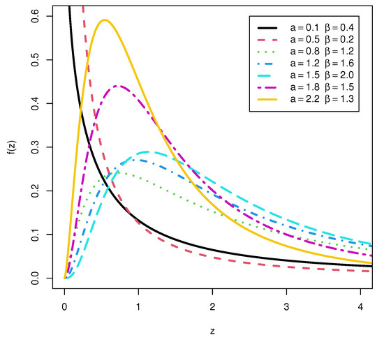
Figure 1. PDF for the TCP-ITL distribution.

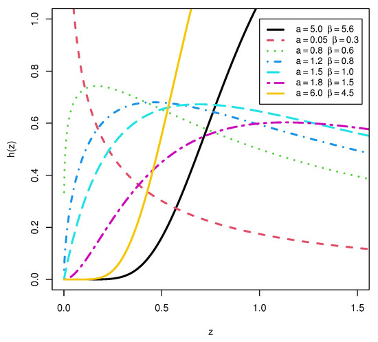
Figure 2. HRF for the TCP-ITL distribution.

3. Properties

This section describes the structural features of the TCPIL as specified in Equation (6), comprising explicit formulas for the QF, the linear representation of the PDF, the rth ordinary and sth incomplete moment, and the moment-generating function. There are also several graphical and numerical representations of these properties.

3.1. Quantile Function

The QF is necessary for generating random variates. For $u\sim uniform(0,1)$, the QF of the TCP-ITL is given by Equation (7). Assume Z∼ TCP-ITL ($a,\beta )$, then its QF is given by Equation (7)

$$Q_u=\frac{\left(1-{\left(1-{\left(tan\left(\frac{\pi u}{4}\right)\right)}^{\frac{1}{\beta }}\right)}^{\frac{1}{a}}\right)+\sqrt{1-{\left(1-{\left(tan\left(\frac{\pi u}{4}\right)\right)}^{\frac{1}{\beta }}\right)}^{\frac{1}{a}}}}{{\left(1-{\left(tan\left(\frac{\pi u}{4}\right)\right)}^{\frac{1}{\beta }}\right)}^{\frac{1}{a}}}.$$

(7)

By replacing $u=0.5$ in Equation (7), the median of the TCP-ITL is readily available. Furthermore, setting $u=0.25$ and $u=0.75$ in (7), the 25th and 75th percentiles are computed. The MacGillivrays skewness ($M{S}_K$) function [30] is computed from the next formula

$$M{S}_K=\frac{z_u+z_{1-u}-2z_{0.5}}{z_u-z_{1-u}},0<u<1.$$

Figure 3 and Figure 4 represent the plots of $M{S}_K$ for some numerous values of the parameters. We may observe that the quantity of $M{S}_K$ rises as $\beta$ and a rise.

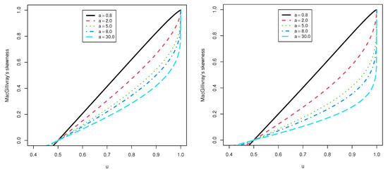
Figure 3. Plots of the MSK for the TCP-ITL distribution at $\beta$ = 0.5 and 1.5.

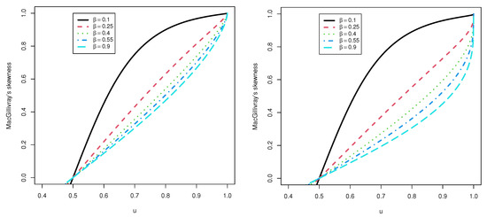
Figure 4. Plots of the MSK for the TCP-ITL distribution at a = 1.5 and 5.0.

3.2. Important Representation

We demonstrated a beneficial increase in the TCP-ITL density that may be utilized to drive various critical TCP-ITL features. According to [2], the PDF given by Equation (6) may be represented as

$$f(z;a,\beta )=\frac{8}{\pi }a\beta z{(1+z)}^{-2a-1}{(1+2z)}^{a-1}\sum _{i=0}^{\infty }{(-1)}^i{\left[1-\frac{{(1+2z)}^a}{{(1+z)}^{2a}}\right]}^{\beta (2+i)-1},$$

(8)

using the next binomial expansion ${(1-z)}^b={\displaystyle \sum _{j=0}^{\infty }}{(-1)}^j\left(\begin{array}{c}b\\ j\end{array}\right)z^j,$ in Equation (8), we obtain

$$f(z;a,\beta )=\frac{8}{\pi }a\beta z\sum _{i,j=0}^{\infty }{(-1)}^{i+j}(i+1)\left(\begin{array}{c}\beta (2+i)-1\\ j\end{array}\right){(1+z)}^{-2a(j+1)-1}{(1+2z)}^{a(j+1)-1},$$

(9)

again using the next binomial expansion ${(1+z)}^b={\displaystyle \sum _{k=0}^{\infty }}\left(\begin{array}{c}b\\ j\end{array}\right)z^j,$ in Equation (9), we obtain

$$f(z;a,\beta )=\sum _{i,j,k=0}^{\infty }{\Delta }_{i,j,k}{z}^{k+1}{(1+z)}^{-2a(j+1)-1},$$

(10)

where ${\Delta }_{i,j,k}=\frac{a\beta }{\pi }{2}^{k+3}{(-1)}^{i+j}(i+1)\left(\begin{array}{c}\beta (2+i)-1\\ j\end{array}\right)\left(\begin{array}{c}a(j+1)-1\\ k\end{array}\right)$.

3.3. The rth Moment

The rth ordinary is an essential statistic for determining the distribution dispersion. To derive the central or actual moments, utilize the following relationship: the first moment about the mean is always equal to zero, and the second moment around the mean is equal to variance as ${\mu }_2={\mu }_2^{\prime }-{\left({\mu }_1^{\prime }\right)}^2$, ${\mu }_3={\mu }_3^{\prime }-3{\mu }_1^{\prime }{\mu }_2^{\prime }+2{\left({\mu }_1^{\prime }\right)}^3$ and ${\mu }_4={\mu }_4^{\prime }-4{\mu }_3^{\prime }{\mu }_1^{\prime }+6{\mu }_2^{\prime }{\left({\mu }_1^{\prime }\right)}^2-3{\left({\mu }_1^{\prime }\right)}^4$. The moment-based measurement of skewness and kurtosis is calculated utilizing ${\beta }_1=\frac{{\mu }_3^2}{{\mu }_2^3}$ and ${\beta }_2=\frac{{\mu }_4}{{\mu }_2^2}$, respectively.

Assume that Z∼ TCP-ITL ($a,\beta$) for $z\in \left(0,\infty \right)$ and $a,\beta >0$, then its rth ordinary by utilizing Equation (6) and beta prime function is $\beta \left(a,b\right)={\int }_0^{\infty }{z}^{a-1}{\left(1+z\right)}^{-a-b}dz$ provided via

$${\mu }_r^{\prime }=\sum _{t=0}^{\infty }{\Delta }_{i,j,k}{\int }_0^{\infty }{z}^{r+k+1}{(1+z)}^{-2a(j+1)-1}dz,$$

$${\mu }_r^{\prime }=\sum _{i,j,k=0}^{\infty }{\Delta }_{i,j,k}\beta \left[\left(r+k+2\right),\left(2a(j+1)-r-k-1\right)\right].$$

(11)

For r = 1, the mean of TCP-ITL is yielded as ${\mu }_1^{\prime }={\sum }_{i,j,k=0}^{\infty }{\Delta }_{i,j,k}\beta \left[k+2,\left(2a(j+1)-k-2\right)\right]$ and $\left[2a(j+1)\right]<k+2$.

Figure 5 depicts the three-dimensional plots of the mean, variance, coefficient of skewness (CS), coefficient of kurtosis (CK), and coefficient of variation (CV) for the TCP-ITL model at $a\in [2,10],\beta \in [1,2]$. Moreover, some numerical values are provided in Table 1. We can notice from Table 1 that when a is fixed and $\beta$ is increasing, then the measures of $E\left(Z\right)$, $E\left(Z^2\right)$, $E\left(Z^3\right)$, $E\left(Z^4\right)$, var are increasing, but the measures of SK, KU, and CV are decreasing. Moreover, when $\beta$ is fixed and a is increasing, then the measures of $E\left(Z\right)$, $E\left(Z^2\right)$, $E\left(Z^3\right)$, $E\left(Z^4\right)$, var, SK, KU, and CV are decreasing.

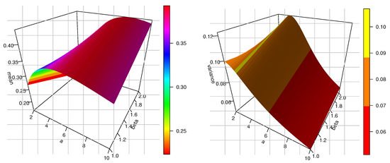
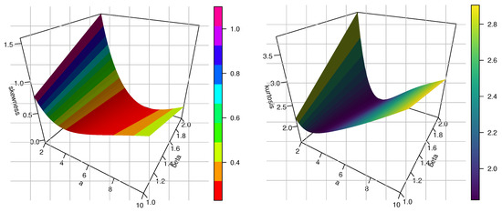
Figure 5. Three-dimensional plots of mean, variance, CS, and CK for the TCP-ITL model at $a\in [2,10],\beta \in [1,2]$.

Table 1. Some numerical values of moments.

a	$\mathit{\beta }$	$\mathit{E}\left(\mathit{Z}\right)$	$\mathit{E}\left({\mathit{Z}}^2\right)$	$\mathit{E}\left({\mathit{Z}}^3\right)$	$\mathit{E}\left({\mathit{Z}}^4\right)$	Variance	Skewness	Kurtosis	Coefficient of Variation
5.0	0.5	0.397	0.422	1.021	6.539	0.264	4.740	75.136	1.293
	0.7	0.506	0.578	1.424	9.152	0.322	4.418	67.225	1.121
	0.9	0.598	0.726	1.823	11.761	0.369	4.238	63.095	1.016
	1.2	0.714	0.936	2.414	15.670	0.426	4.084	59.709	0.915
	1.5	0.811	1.133	2.995	19.571	0.475	3.994	57.819	0.849
	2.0	0.948	1.439	3.946	26.054	0.541	3.908	56.075	0.777
	2.5	1.061	1.722	4.874	32.515	0.597	3.859	55.127	0.729
	3.0	1.158	1.986	5.783	38.953	0.646	3.828	54.550	0.694
6.0	0.5	0.343	0.290	0.489	1.624	0.172	3.799	37.659	1.210
	0.7	0.435	0.395	0.681	2.272	0.206	3.519	33.601	1.045
	0.9	0.512	0.495	0.870	2.918	0.233	3.363	31.500	0.943
	1.2	0.609	0.635	1.148	3.884	0.265	3.229	29.796	0.845
	1.5	0.689	0.766	1.421	4.845	0.290	3.152	28.858	0.781
	2.0	0.801	0.966	1.863	6.439	0.325	3.078	28.009	0.711
	2.5	0.893	1.150	2.292	8.020	0.353	3.037	27.560	0.665
	3.0	0.971	1.319	2.708	9.589	0.376	3.012	27.295	0.632
7.0	0.5	0.304	0.217	0.286	0.655	0.124	3.303	26.152	1.156
	0.7	0.385	0.295	0.397	0.915	0.147	3.044	23.290	0.995
	0.9	0.452	0.368	0.507	1.175	0.164	2.899	21.819	0.895
	1.2	0.536	0.471	0.667	1.563	0.184	2.776	20.636	0.800
	1.5	0.605	0.566	0.824	1.948	0.199	2.705	19.993	0.737
	2.0	0.701	0.710	1.077	2.584	0.220	2.638	19.421	0.669
	2.5	0.778	0.842	1.320	3.212	0.236	2.601	19.126	0.624
	3.0	0.845	0.962	1.554	3.834	0.249	2.579	18.957	0.591

3.4. The sth Incomplete Moment

The sth incomplete moment is a significant metric with several uses, including calculating the mean waiting time, conditional moments, and income inequality measures.

Assume that Z∼ TCP-ITL ($a,\beta$) for $z\in \left(0,\infty \right)$ and $a,\beta >0$, then its sth incomplete moments by utilizing (6) and incomplete beta function ${\beta }_w\left(a,b\right)={\int }_0^w{z}^{a-1}{\left(1-z\right)}^{b-1}dz$ are provided via

$${\phi }_s\left(w\right)=\sum _{i,j,k=0}^{\infty }{\Delta }_{i,j,k}{\beta }_{\frac{w}{1+w}}\left[\left(s+k+1\right),\left(2a(j+1)-s-k-1\right)\right].$$

(12)

Theoretically, Equation (12) is beneficial by utilizing the relationship between incomplete beta and Gauss hypergeometric functions as ${\beta }_z\left(a,b\right)=\frac{z^a}{a}{}_2{F}_1\left(a,1-b;a+1;z\right)$. The readers are referred to [31] for a more extensive examination of the numerous beta functions and their relationships.

$${\phi }_s\left(w\right)=\sum _{i,j,k=0}^{\infty }{\Delta }_{i,j,k}\frac{{\left(\frac{w}{1+w}\right)}^{s+k+1}}{\left(s+k+1\right)}{}_2{F}_1\left[s+k+1,1-2a(j+1)+s+k;s+k+2;\frac{w}{1+w}\right].$$

3.5. Moment-Generating Function

According to the definition, the moment-generating function $M\left(t\right)=E\left[e^{tZ}\right]=\int e^{tz}f\left(z\right)dz$, can be yielded. Assume that Z∼ TCP-ITL ($a,\beta$) for $z\in \left(0,\infty \right)$ and $a,\beta >0$, then its moment-generating function may be computed by utilizing (6) and replacing $e^{tz}={\sum }_{m=0}^{\infty }\frac{t^m}{m!}{z}^m$ and is provided via

$$E\left[e^{tZ}\right]=\sum _{m=0}^{\infty }\sum _{i,j,k=0}^{\infty }{\Delta }_{i,j,k}\frac{t^m}{m!}\beta \left[m+k+1,\left(2a(j+1)-m-k-1\right)\right],$$

(13)

where $\left[2a(j+1)\right]<m+k+1$.

4. Entropy Measures

Entropies are a measurement of the variation, instability, or unpredictability of a system.

4.1. The R$\acute{e}$nyi Entropy

The R$\acute{e}$nyi entropy (RE) [32] is used in ecology and statistics as a measure of diversity. It is identified by the expression for $\nu >0$ and $\nu \ne 1$.

$$I_{\nu }\left(Z\right)={(1-\nu )}^{-1}log{\int }_0^{+\infty }f{\left(z\right)}^{\nu }dz.$$

(14)

We employ the same series expansions and mathematical manipulation that we used to calculate Equation (6) to achieve

$$I_{\nu }\left(Z\right)={(1-\nu )}^{-1}log\left[\sum _{i,j,k=0}^{\infty }{\omega }_{i,j,k}\beta \left[\nu +k+1,2a(j+\nu )-k-1\right]\right],$$

where

${\omega }_{i,j,k}={\left(\frac{a\beta }{\pi }\right)}^{\nu }{2}^{k+3\nu }{(-1)}^{i+j}\left(\begin{array}{c}\nu +i-1\\ i\end{array}\right)\left(\begin{array}{c}\nu (\beta -1)+2\beta i\\ j\end{array}\right)\left(\begin{array}{c}\nu (a-1)+aj\\ k\end{array}\right)$.

4.2. Havrda and Charvat Entropy

The Havrda and Charvat entropy (HCE) [33] measure is provided via

$$H{C}_{\nu }\left(x\right)=\frac{1}{2^{1-\nu }-1}\left[{\left({\displaystyle {\int }_0^{+\infty }}{\left(f\left(x\right)\right)}^{\nu }dx\right)}^{\frac{1}{\nu }}-1\right],\nu >0,\nu \ne 1.$$

(15)

For the TCP-ITL distribution, the Havrda and Charvat entropy is obtained as

$$H{C}_{\nu }\left(x\right)=\frac{1}{2^{1-\nu }-1}\left[{\left(\sum _{i,j,k=0}^{\infty }{\omega }_{i,j,k}\beta \left[\nu +k+1,2a(j+\nu )-k-1\right]\right)}^{\frac{1}{\nu }}-1\right].$$

4.3. Tsallis Entropy

The Tsallis entropy (TE) [34] measure is provided via

$$T_{\nu }\left(x\right)=\frac{1}{\nu -1}\left[1-{\displaystyle {\int }_0^{+\infty }}{\left(f\left(x\right)\right)}^{\nu }dx\right],\nu >0,\nu \ne 1.$$

(16)

For the TCP-ITL distribution, the Tsallis entropy is obtained as

$$T_{\nu }\left(x\right)=\frac{1}{\nu -1}\left[1-\sum _{i,j,k=0}^{\infty }{\omega }_{i,j,k}\beta \left[\nu +k+1,2a(j+\nu )-k-1\right]\right].$$

4.4. Arimoto Entropy

The Arimoto entropy (AE) [35] measure is provided via

$$A_{\nu }\left(x\right)=\frac{\nu }{1-\nu }\left[{\left({\displaystyle {\int }_0^{+\infty }}{\left(f\left(x\right)\right)}^{\nu }dx\right)}^{\frac{1}{\nu }}-1\right],\nu >0,\nu \ne 1.$$

(17)

For the TCP-ITL distribution, the Arimoto entropy is obtained as

$$A_{\nu }\left(x\right)=\frac{\nu }{1-\nu }\left[{\left(\sum _{i,j,k=0}^{\infty }{\omega }_{i,j,k}\beta \left[\nu +k+1,2a(j+\nu )-k-1\right]\right)}^{\frac{1}{\nu }}-1\right].$$

Some numerical values of entropy are provided in Table 2 and Table 3. We can notice from Table 2 and Table 3 the following comments:

• When a and $\beta$ are fixed and $\nu$ is increasing, then the measures of RE, HCE, TE, and AE are decreasing.
• When a and $\nu$ are fixed and $\beta$ is increasing, then the measures of RE, HCE, TE, and AE are increasing.
• When $\nu$ and $\beta$ are fixed and a is increasing, then the measures of RE, HCE, TE, and AE are decreasing.

Table 2. Some numerical values of entropy at $\nu =0.8,1.5$.

a	$\mathit{\beta }$	$\mathit{\nu }=0.8$				$\mathit{\nu }=1.5$
		R$\acute{\mathit{e}}$nyi	Havrda and Charvat	Tsallis	Arimoto	R$\acute{\mathit{e}}$nyi	Havrda and Charvat	Tsallis	Arimoto
5.0	0.5	0.098	0.311	0.233	0.231	−0.087	−0.360	−0.208	−0.211
	0.7	0.189	0.612	0.460	0.455	0.035	0.135	0.080	0.079
	0.9	0.243	0.797	0.601	0.593	0.100	0.370	0.221	0.217
	1.2	0.294	0.977	0.739	0.726	0.157	0.565	0.341	0.331
	1.5	0.328	1.098	0.832	0.816	0.194	0.683	0.415	0.400
	2.0	0.367	1.238	0.941	0.920	0.235	0.808	0.494	0.473
	2.5	0.394	1.337	1.018	0.994	0.262	0.890	0.547	0.522
	3.0	0.414	1.413	1.077	1.051	0.283	0.951	0.587	0.557
6.0	0.5	0.032	0.101	0.075	0.075	−0.140	−0.599	−0.342	−0.351
	0.7	0.119	0.378	0.283	0.281	−0.024	−0.095	−0.055	−0.056
	0.9	0.169	0.545	0.409	0.405	0.036	0.140	0.082	0.082
	1.2	0.216	0.703	0.529	0.523	0.089	0.331	0.197	0.194
	1.5	0.246	0.808	0.609	0.600	0.121	0.445	0.267	0.261
	2.0	0.280	0.926	0.700	0.688	0.157	0.564	0.340	0.330
	2.5	0.303	1.007	0.762	0.749	0.181	0.641	0.389	0.376
	3.0	0.320	1.069	0.810	0.795	0.199	0.698	0.424	0.409
7.0	0.5	−0.021	−0.065	−0.048	−0.048	−0.185	−0.809	−0.457	−0.474
	0.7	0.062	0.195	0.145	0.145	−0.072	−0.297	−0.171	−0.174
	0.9	0.110	0.348	0.260	0.259	−0.016	−0.062	−0.036	−0.036
	1.2	0.153	0.490	0.368	0.365	0.033	0.127	0.075	0.074
	1.5	0.181	0.583	0.438	0.433	0.063	0.237	0.141	0.139
	2.0	0.211	0.685	0.516	0.509	0.094	0.350	0.209	0.205
	2.5	0.231	0.754	0.569	0.561	0.115	0.423	0.253	0.248
	3.0	0.246	0.806	0.608	0.600	0.130	0.475	0.285	0.278

Table 2. Some numerical values of entropy at $\nu =0.8,1.5$.

a	$\mathit{\beta }$	$\mathit{\nu }=0.8$				$\mathit{\nu }=1.5$
		R$\acute{\mathit{e}}$nyi	Havrda and Charvat	Tsallis	Arimoto	R$\acute{\mathit{e}}$nyi	Havrda and Charvat	Tsallis	Arimoto
5.0	0.5	0.098	0.311	0.233	0.231	−0.087	−0.360	−0.208	−0.211
	0.7	0.189	0.612	0.460	0.455	0.035	0.135	0.080	0.079
	0.9	0.243	0.797	0.601	0.593	0.100	0.370	0.221	0.217
	1.2	0.294	0.977	0.739	0.726	0.157	0.565	0.341	0.331
	1.5	0.328	1.098	0.832	0.816	0.194	0.683	0.415	0.400
	2.0	0.367	1.238	0.941	0.920	0.235	0.808	0.494	0.473
	2.5	0.394	1.337	1.018	0.994	0.262	0.890	0.547	0.522
	3.0	0.414	1.413	1.077	1.051	0.283	0.951	0.587	0.557
6.0	0.5	0.032	0.101	0.075	0.075	−0.140	−0.599	−0.342	−0.351
	0.7	0.119	0.378	0.283	0.281	−0.024	−0.095	−0.055	−0.056
	0.9	0.169	0.545	0.409	0.405	0.036	0.140	0.082	0.082
	1.2	0.216	0.703	0.529	0.523	0.089	0.331	0.197	0.194
	1.5	0.246	0.808	0.609	0.600	0.121	0.445	0.267	0.261
	2.0	0.280	0.926	0.700	0.688	0.157	0.564	0.340	0.330
	2.5	0.303	1.007	0.762	0.749	0.181	0.641	0.389	0.376
	3.0	0.320	1.069	0.810	0.795	0.199	0.698	0.424	0.409
7.0	0.5	−0.021	−0.065	−0.048	−0.048	−0.185	−0.809	−0.457	−0.474
	0.7	0.062	0.195	0.145	0.145	−0.072	−0.297	−0.171	−0.174
	0.9	0.110	0.348	0.260	0.259	−0.016	−0.062	−0.036	−0.036
	1.2	0.153	0.490	0.368	0.365	0.033	0.127	0.075	0.074
	1.5	0.181	0.583	0.438	0.433	0.063	0.237	0.141	0.139
	2.0	0.211	0.685	0.516	0.509	0.094	0.350	0.209	0.205
	2.5	0.231	0.754	0.569	0.561	0.115	0.423	0.253	0.248
	3.0	0.246	0.806	0.608	0.600	0.130	0.475	0.285	0.278

Table 3. Some numerical values of entropy at $\nu =2.0,2.5$.

a	$\mathit{\beta }$	$\mathit{\nu }=2.0$				$\mathit{\nu }=2.5$
		R$\acute{\mathit{e}}$nyi	Havrda and Charvat	Tsallis	Arimoto	R$\acute{\mathit{e}}$nyi	Havrda and Charvat	Tsallis	Arimoto
5.0	0.5	−0.150	−0.826	−0.377	−0.413	−0.192	−1.452	−0.654	−0.626
	0.7	−0.015	−0.069	−0.034	−0.034	−0.047	−0.270	−0.140	−0.116
	0.9	0.053	0.231	0.119	0.116	0.024	0.121	0.066	0.052
	1.2	0.113	0.457	0.243	0.229	0.084	0.389	0.225	0.168
	1.5	0.150	0.585	0.318	0.292	0.122	0.531	0.316	0.229
	2.0	0.191	0.713	0.396	0.356	0.163	0.667	0.410	0.287
	2.5	0.220	0.794	0.447	0.397	0.192	0.749	0.470	0.323
	3.0	0.241	0.851	0.484	0.426	0.213	0.805	0.513	0.347
6.0	0.5	−0.200	−1.171	−0.518	−0.586	−0.240	−1.994	−0.855	−0.860
	0.7	−0.071	−0.354	−0.170	−0.177	−0.101	−0.646	−0.318	−0.278
	0.9	−0.007	−0.034	−0.017	−0.017	−0.036	−0.203	−0.106	−0.088
	1.2	0.047	0.204	0.105	0.102	0.019	0.099	0.054	0.043
	1.5	0.080	0.336	0.176	0.168	0.053	0.258	0.145	0.111
	2.0	0.116	0.468	0.250	0.234	0.089	0.409	0.237	0.176
	2.5	0.140	0.551	0.298	0.275	0.113	0.500	0.296	0.216
	3.0	0.158	0.609	0.332	0.305	0.131	0.563	0.338	0.243
7.0	0.5	−0.242	−1.491	−0.642	−0.745	−0.280	−2.523	−1.037	−1.087
	0.7	−0.117	−0.619	−0.289	−0.309	−0.146	−1.016	−0.479	−0.438
	0.9	−0.057	−0.282	−0.136	−0.141	−0.085	−0.525	−0.262	−0.226
	1.2	−0.007	−0.034	−0.017	−0.017	−0.034	−0.192	−0.100	−0.083
	1.5	0.023	0.102	0.052	0.051	−0.003	−0.019	−0.010	−0.008
	2.0	0.055	0.236	0.122	0.118	0.029	0.145	0.080	0.063
	2.5	0.076	0.319	0.167	0.160	0.050	0.244	0.137	0.105
	3.0	0.091	0.378	0.199	0.189	0.065	0.311	0.177	0.134

Table 3. Some numerical values of entropy at $\nu =2.0,2.5$.

a	$\mathit{\beta }$	$\mathit{\nu }=2.0$				$\mathit{\nu }=2.5$
		R$\acute{\mathit{e}}$nyi	Havrda and Charvat	Tsallis	Arimoto	R$\acute{\mathit{e}}$nyi	Havrda and Charvat	Tsallis	Arimoto
5.0	0.5	−0.150	−0.826	−0.377	−0.413	−0.192	−1.452	−0.654	−0.626
	0.7	−0.015	−0.069	−0.034	−0.034	−0.047	−0.270	−0.140	−0.116
	0.9	0.053	0.231	0.119	0.116	0.024	0.121	0.066	0.052
	1.2	0.113	0.457	0.243	0.229	0.084	0.389	0.225	0.168
	1.5	0.150	0.585	0.318	0.292	0.122	0.531	0.316	0.229
	2.0	0.191	0.713	0.396	0.356	0.163	0.667	0.410	0.287
	2.5	0.220	0.794	0.447	0.397	0.192	0.749	0.470	0.323
	3.0	0.241	0.851	0.484	0.426	0.213	0.805	0.513	0.347
6.0	0.5	−0.200	−1.171	−0.518	−0.586	−0.240	−1.994	−0.855	−0.860
	0.7	−0.071	−0.354	−0.170	−0.177	−0.101	−0.646	−0.318	−0.278
	0.9	−0.007	−0.034	−0.017	−0.017	−0.036	−0.203	−0.106	−0.088
	1.2	0.047	0.204	0.105	0.102	0.019	0.099	0.054	0.043
	1.5	0.080	0.336	0.176	0.168	0.053	0.258	0.145	0.111
	2.0	0.116	0.468	0.250	0.234	0.089	0.409	0.237	0.176
	2.5	0.140	0.551	0.298	0.275	0.113	0.500	0.296	0.216
	3.0	0.158	0.609	0.332	0.305	0.131	0.563	0.338	0.243
7.0	0.5	−0.242	−1.491	−0.642	−0.745	−0.280	−2.523	−1.037	−1.087
	0.7	−0.117	−0.619	−0.289	−0.309	−0.146	−1.016	−0.479	−0.438
	0.9	−0.057	−0.282	−0.136	−0.141	−0.085	−0.525	−0.262	−0.226
	1.2	−0.007	−0.034	−0.017	−0.017	−0.034	−0.192	−0.100	−0.083
	1.5	0.023	0.102	0.052	0.051	−0.003	−0.019	−0.010	−0.008
	2.0	0.055	0.236	0.122	0.118	0.029	0.145	0.080	0.063
	2.5	0.076	0.319	0.167	0.160	0.050	0.244	0.137	0.105
	3.0	0.091	0.378	0.199	0.189	0.065	0.311	0.177	0.134

5. Model Inference and Estimation Method

Hybrid censoring is discussed briefly in this section. Assume that n test units are uniformly distributed with the PDF $f(z;\mathrm{\Theta })$ and that $\mathrm{\Theta }$ is a vector of unknown parameters. Let $z_{1:n}<z_{2:n}<\cdots <z_{n:n}$ represent the ordered s of these test units. Remember that a life test experiment is ended under hybrid censoring when either a pre-specified time T or a pre-determined r number of units fail. In this scenario, an experiment is to be stopped at a random time point $\kappa$, where $\kappa =minimal(T;z_{r:n})$. As a result, the observed lifespan under this censorship could fall into one of three categories:

Category I:

$z_{1:n}<z_{2:n}<\cdots <z_{d:n}$, if $d<r$ and $z_{d:n}<T<z_{d+1:n}$ (type-I censored).

Category II:

$z_{1:n}<z_{2:n}<\cdots <z_{r:n}$, if $z_{r:n}<T$ (type-II censored).

Category III:

$z_{1:n}<z_{2:n}<\cdots <z_{n:n}$, if $z_{n:n}<T$ and $n=r$ (complete sample).

Notice that Category I, Category II, and Category III, respectively, correspond to the type-I, type-II censoring, and complete sample. Then, $(z_{1:n}<z_{2:n}<\cdots <z_{d:n})$ is a censored hybrid sample with the PDF $f(z;\mathrm{\Theta })$ and the CDF $F(z;\mathrm{\Theta })$ describing its distribution. The corresponding likelihood function can then be expressed as

$$L\left(\mathrm{\Theta }\right)\propto {\left[1-F(\kappa ;a,\beta )\right]}^{n-d}\prod _{i=1}^{d}f(z;a,\beta )$$

For more information on the hybrid censoring sample, see Balakrishnan and Kundu [36]. For more information examples, see [37]’s obtained Bayesian estimation and prediction for a hybrid censored lognormal distribution.

To evaluate the estimation problem of the TCP-ITL distribution based on hybrid censoring samples, this part uses three estimate methods: the maximum likelihood, maximum product of spacing, and Bayesian.

5.1. Maximum Likelihood Estimation

The maximum likelihood estimators (MLEs) of the TCP-ITL distribution were investigated. It was worked as the case when both $\mathrm{\Theta }=(a,\beta )$ are unknown. Suppose that $z_1,\cdots ,z_n$ be a random sample from the TCP-ITL distribution and assume that $\mathrm{\Theta }=(a,\beta )$ be the parameter vector. The likelihood function of the TCP-ITL distribution under the hybrid censored samples takes the form

$$\begin{array}{cc}\hfill L_n\left(\mathrm{\Theta }\right)=& {\left(\frac{8}{\pi }\right)}^n{a}^n{\beta }^n\prod _{i=1}^n{z}_i{(1+z_i)}^{-2a-1}{(1+2z_i)}^{a-1}\frac{{\left[1-\left\{\frac{{(1+2z_i)}^a}{{(1+z_i)}^{2a}}\right\}\right]}^{\beta -1}}{\left[1+{\left(1-\left\{\frac{{(1+2z_i)}^a}{{(1+z_i)}^{2a}}\right\}\right)}^{2\beta }\right]}\times \hfill \\ & {\left[1-\frac{4}{\pi }arctan{\left[1-\left\{\frac{{(1+2\kappa )}^a}{{(1+\kappa )}^{2a}}\right\}\right]}^{\beta }\right]}^{n-d},\hfill \end{array}$$

(18)

The log-likelihood $(\ell )$ function is defined as follows:

$$\begin{array}{cc}\hfill {\ell }_n\left(\mathrm{\Theta }\right)=& n\left[ln\left(\frac{8}{\pi }\right)+ln\left(a\right)+ln\left(\beta \right)\right]+\sum _{i=1}^{n}ln\left(z_i\right)-(2a+1)\sum _{i=1}^{n}ln(1+z_i)+(a-1)\sum _{i=1}^{n}ln(1+2z_i)+\hfill \\ & (\beta -1)\sum _{i=1}^{n}ln\left[1-\left\{\frac{{(1+2z_i)}^a}{{(1+z_i)}^{2a}}\right\}\right]-\sum _{i=1}^{n}ln\left[1+{\left(1-\left\{\frac{{(1+2z_i)}^a}{{(1+z_i)}^{2a}}\right\}\right)}^{2\beta }\right]\hfill \\ & +\left(n-d\right)ln\left[1-\frac{4}{\pi }arctan{\left[1-\left\{\frac{{(1+2\kappa )}^a}{{(1+\kappa )}^{2a}}\right\}\right]}^{\beta }\right],\hfill \end{array}$$

(19)

The components of score vector $U_n\left(\mathrm{\Theta }\right)=\frac{\partial {\ell }_n\left(\mathrm{\Theta }\right)}{\partial \mathrm{\Theta }}=\left(\frac{\partial {\ell }_n\left(\mathrm{\Theta }\right)}{\partial a},\frac{\partial {\ell }_n\left(\mathrm{\Theta }\right)}{\partial \beta }\right)$ are given below

$$\begin{array}{cc}\hfill U_a\left(\mathrm{\Theta }\right)=& \frac{\partial {\ell }_n\left(\mathrm{\Theta }\right)}{\partial a}=\frac{n}{a}-2\sum _{i=1}^{n}ln(1+z_i)+\sum _{i=1}^{n}ln(1+2z_i)+(\beta -1)\sum _{i=1}^n\frac{{\left\{\frac{(1+2z_i)}{{(1+z_i)}^2}\right\}}^{a}ln\left\{\frac{(1+2z_i)}{{(1+z_i)}^2}\right\}}{1-{\left\{\frac{(1+2z_i)}{{(1+z_i)}^2}\right\}}^a}+\hfill \\ & 2\beta \sum _{i=1}^n\frac{{\left(1-{\left\{\frac{(1+2z_i)}{{(1+z_i)}^2}\right\}}^a\right)}^{2\beta -1}{\left\{\frac{(1+2z_i)}{{(1+z_i)}^2}\right\}}^{a}ln\left\{\frac{(1+2z_i)}{{(1+z_i)}^2}\right\}}{1+{\left(1-{\left\{\frac{(1+2z_i)}{{(1+z_i)}^2}\right\}}^a\right)}^{4\beta }}\hfill \\ & +\frac{4\beta (n-d){\left\{\frac{1+2\kappa }{{\left(1+2\kappa \right)}^2}\right\}}^a{\left[1-{\left\{\frac{1+2\kappa }{{\left(1+2\kappa \right)}^2}\right\}}^a\right]}^{\beta -1}ln\left[\frac{1+2\kappa }{{\left(1+2\kappa \right)}^2}\right]}{\left(\pi -4arctan{\left[1-{\left\{\frac{1+2\kappa }{{\left(1+2\kappa \right)}^2}\right\}}^a\right]}^{\beta }\right)\left(1+{\left[1-{\left\{\frac{1+2\kappa }{{\left(1+2\kappa \right)}^2}\right\}}^a\right]}^{2\beta }\right)},\hfill \end{array}$$

(20)

and

$$\begin{array}{ccc}\hfill U_{\beta }\left(\mathrm{\Theta }\right)& =& \frac{\partial L_n\left(\mathrm{\Theta }\right)}{\partial \beta }=\frac{n}{\beta }-\frac{4(n-d){\left[1-{\left\{\frac{1+2\kappa }{{\left(1+2\kappa \right)}^2}\right\}}^a\right]}^{\beta }ln\left[1-{\left\{\frac{1+2\kappa }{{\left(1+2\kappa \right)}^2}\right\}}^a\right]}{\left(\pi -4arctan{\left[1-{\left\{\frac{1+2\kappa }{{\left(1+2\kappa \right)}^2}\right\}}^a\right]}^{\beta }\right)\left(1+{\left[1-{\left\{\frac{1+2\kappa }{{\left(1+2\kappa \right)}^2}\right\}}^a\right]}^{2\beta }\right)}.\hfill \end{array}$$

(21)

To produce the MLE, two nonlinear systems of equations that are differentiating (20) and (21) with respect to $\alpha$ and $\beta$ and equating each solution to zero must be solved concurrently. By using the ’maxLik’ package, which uses the Newton–Rabson (NR) method of maximization in the maximum likelihood computations, one can utilize the R statistical programming language software to calculate the desired MLEs $\alpha$ and $\beta$ for any given data set.

5.2. Maximum Product of Spacing Method

If $z_{\left(1\right)}<\cdots <z_{\left(n\right)}$ is a random sample of the size n, you can describe the uniform spacing as:

$$D_i\left(\mathrm{\Theta }\right)=F(z_{\left(i\right)},\mathrm{\Theta })-F(z_{(i-1)},\mathrm{\Theta });i=1,\dots ,n+1,$$

(22)

where $D_i\left(\mathrm{\Theta }\right)$ denotes the uniform spacings, $F(z_{\left(0\right)},\mathrm{\Theta })=0$, $F(z_{(n+1)},\mathrm{\Theta })=1$, and ${\sum }_{i=1}^{n+1}{D}_i\left(\mathrm{\Theta }\right)=1$. This is the general form of MPS with hybrid censored samples.

$$PS\left(\mathrm{\Theta }\right)\propto {\left[1-F(\kappa ,\mathrm{\Theta })\right]}^{n-d}\prod _{i=1}^{d+1}{D}_i\left(\mathrm{\Theta }\right)$$

(23)

The maximum product of spacing (MPS) estimators (MPSE) of the TCP-ITL distribution parameters based on hybrid censored samples can be obtained by maximizing

$$\begin{array}{cc}\hfill PS\left(\mathrm{\Theta }\right)\propto & \prod _{i=1}^{d+1}\left\{\frac{4}{\pi }arctan{\left[1-\left\{\frac{{(1+2z_i)}^a}{{(1+z_i)}^{2a}}\right\}\right]}^{\beta }-\frac{4}{\pi }arctan{\left[1-\left\{\frac{{(1+2z_{i-1})}^a}{{(1+z_{i-1})}^{2a}}\right\}\right]}^{\beta }\right\}\hfill \\ & {\left[1-\frac{4}{\pi }arctan{\left[1-\left\{\frac{{(1+2\kappa )}^a}{{(1+\kappa )}^{2a}}\right\}\right]}^{\beta }\right]}^{n-d}\hfill \end{array}$$

(24)

with respect to a and $\beta$. Further, the MPSE of the TCP-ITL distribution can also be obtained by solving the nonlinear equation of derivatives of $ln\left[PS\left(\mathrm{\Theta }\right)\right]$ with respect to $a,$ and $\beta$.

5.3. Bayesian Estimation

In this subsection, the Bayesian estimation of the parameter of the model is obtained when data are observed based on the squared error loss function (SELF), which is defined by

$$\begin{array}{cc}\hfill L_{SELF}=(\mathrm{\Theta },\check{\mathrm{\Theta }})& ={(\check{\mathrm{\Theta }}-\mathrm{\Theta })}^2,\hfill \end{array}$$

where $\check{\mathrm{\Theta }}$ is an estimator of $\mathrm{\Theta }$. Denote the prior and posterior distributions of $\mathrm{\Theta }$ by $\pi \left(\mathrm{\Theta }\right)$ and ${\pi }^{*}(\mathrm{\Theta }\mid \underline{x})$, respectively. Under the SELF, the Bayesian estimation of any function $B\left(\mathrm{\Theta }\right)$ of $\mathrm{\Theta }$ is given by

$$\begin{array}{cc}\hfill {\tilde{v}}_{SELF}& =E[\mathrm{\Theta }\mid \underline{x}]={\int }_0^{\infty }{\int }_0^{\infty }\mathrm{\Theta }{\pi }^{*}(\mathrm{\Theta }\mid \underline{x})dad\beta .\hfill \end{array}$$

(25)

Prior distribution is important for the development of Bayes estimators.

Under the assumption of gamma prior distributions, we investigate this estimate problem. Therefore, it is assumed here that a and $\beta$ follow independent gamma distributions with $a\sim \Gamma ({\eta }_1,b_1)$, and $\beta \sim \Gamma ({\eta }_2,b_2)$, with probability densities given by, respectively,

$$\begin{array}{c}\hfill \pi \left(a\right)\propto a^{{\eta }_1-1}{e}^{-\frac{a}{b_1}},\pi \left(\beta \right)\propto {\beta }^{{\eta }_2-1}{e}^{-\frac{\beta }{b_2}},a,\beta >0,{\eta }_i,b_i>0,i=1,2.\end{array}$$

(26)

Using the informative prior (26) and the likelihood function (18), the joint posterior density can be derived as follows:

$$\begin{array}{cc}\hfill {\mathrm{\Pi }}^{*}\left(\mathrm{\Theta }\right)\propto & a^{n+{\eta }_1-1}{e}^{-\frac{a}{b_1}}{\beta }^{n+{\eta }_2-1}{e}^{-\frac{\beta }{b_2}}\prod _{i=1}^n{z}_i{(1+z_i)}^{-2a-1}{(1+2z_i)}^{a-1}\frac{{\left[1-\left\{\frac{{(1+2z_i)}^a}{{(1+z_i)}^{2a}}\right\}\right]}^{\beta -1}}{\left[1+{\left(1-\left\{\frac{{(1+2z_i)}^a}{{(1+z_i)}^{2a}}\right\}\right)}^{2\beta }\right]}\times \hfill \\ & {\left[1-\frac{4}{\pi }arctan{\left[1-\left\{\frac{{(1+2\kappa )}^a}{{(1+\kappa )}^{2a}}\right\}\right]}^{\beta }\right]}^{n-d}.\hfill \end{array}$$

(27)

The marginal posterior densities of the parameters a and $\beta$ can be derived as

$$\left\{\begin{array}{cc}\hfill {\pi }^{*}\left(a\right)& \propto a^{n+{\eta }_1-1}{e}^{-\frac{a}{b_1}}\prod _{i=1}^n{(1+z_i)}^{-2a-1}{(1+2z_i)}^{a-1}\frac{{\left[1-\left\{\frac{{(1+2z_i)}^a}{{(1+z_i)}^{2a}}\right\}\right]}^{\beta -1}}{\left[1+{\left(1-\left\{\frac{{(1+2z_i)}^a}{{(1+z_i)}^{2a}}\right\}\right)}^{2\beta }\right]}\times \hfill \\ & {\left[1-\frac{4}{\pi }arctan{\left[1-\left\{\frac{{(1+2\kappa )}^a}{{(1+\kappa )}^{2a}}\right\}\right]}^{\beta }\right]}^{n-d}\hfill \\ \hfill {\pi }^{*}\left(\beta \right)& \propto {\beta }^{n+{\eta }_2-1}{e}^{-\frac{\beta }{b_2}}\prod _{i=1}^n\frac{{\left[1-\left\{\frac{{(1+2z_i)}^a}{{(1+z_i)}^{2a}}\right\}\right]}^{\beta -1}}{\left[1+{\left(1-\left\{\frac{{(1+2z_i)}^a}{{(1+z_i)}^{2a}}\right\}\right)}^{2\beta }\right]}{\left[1-\frac{4}{\pi }arctan{\left[1-\left\{\frac{{(1+2\kappa )}^a}{{(1+\kappa )}^{2a}}\right\}\right]}^{\beta }\right]}^{n-d}\hfill \end{array}\right.$$

(28)

Because the marginal posterior densities in (28) are not well-known distributions, we will utilize the Metropolis–Hastings sampler to produce values for a and $\beta$ using the normal proposal distribution in (28).

Furthermore, Chen and Shao’s [38] approach was widely used to create the highest posterior density (HPD) intervals for the Bayesian estimation with uncertain benefit distribution parameters. For example, using two endpoints from the MCMC sample outputs, $2.5\%$ and $97.5\%$ percentiles, a $95\%$ HPD interval can be produced. The Bayes trustworthy intervals for the $\beta ,\theta$, and $\delta$ parameters are calculated as follows:

• Sorted parameters as ${\tilde{a}}^{\left[1\right]}<{\tilde{a}}^{\left[2\right]}<\dots <{\tilde{a}}^{\left[N\right]}$, and ${\tilde{\beta }}^{\left[1\right]}<{\tilde{\beta }}^{\left[2\right]}<\dots <{\tilde{\beta }}^{\left[N\right]}$, and N is the length of MCMC generated.
• The $95\%$ symmetric credible intervals of $\tilde{a}$ and $\tilde{\beta }$ become $\left({\tilde{a}}^{L\frac{25}{1000}},{\tilde{a}}^{L\frac{975}{1000}}\right)$ and $\left({\tilde{\beta }}^{L\frac{25}{1000}},{\tilde{\beta }}^{L\frac{975}{1000}}\right)$.

6. Simulation

In this section, we conduct a simulation study to compare the performance of the proposed methods. We first simulate the hybrid censored data from the TCP-ITL distribution for different choices of n and r for all cases as:

If $n=50$, $r=25,35$, and 50. While $n=100$, $r=70,85$, and 100.

The time of the hybrid censored sample was changed for each case as follows:

In Table 4: If $T=15,40$, and 9999 when $a=0.35,\beta =1.5$. If $T=2.3,3.7$, and 999 when $a=1.2,\beta =1.5$. If $T=1,1.7$, and 99 when $a=3,\beta =1.5$.

Table 4. MSE and length of CI for MLE, MPS, and Bayesian estimation for parameter of the TCP-ITL based on hybrid censored samples: when $\beta =1.5$.

	$\mathit{\beta }=1.5$		n = 50		MLE		MPS		Bayesian
n	$\mathit{a}$	T	r		MSE	L.ACI	MSE	L.ACI	MSE	L.CCI
	0.35	15	25	a	0.0237	0.5321	0.0191	0.5331	0.0137	0.2798
				$\beta$	0.2496	1.5783	0.1684	1.5839	0.0253	0.5015
		40	35	a	0.0133	0.4077	0.0111	0.4076	0.0130	0.2333
				$\beta$	0.1735	1.3588	0.1248	1.3582	0.0186	0.4117
		9999	50	a	0.0068	0.2867	0.0059	0.2869	0.0051	0.1909
				$\beta$	0.1107	1.0833	0.0830	1.0840	0.0083	0.3070
50	1.2	2.3	25	a	0.2271	1.6155	0.1731	1.6163	0.0191	0.4758
				$\beta$	0.2692	1.5965	0.1701	1.5975	0.0193	0.4719
		3.7	35	a	0.1157	1.2142	0.1009	1.2137	0.0147	0.4122
				$\beta$	0.1694	1.3425	0.1251	1.3425	0.0163	0.4217
		999	50	a	0.0569	0.8291	0.0506	0.8288	0.0086	0.2957
				$\beta$	0.1002	1.0259	0.0780	1.0256	0.0078	0.3024
	3	1	25	a	1.2864	3.8258	0.9727	3.8240	0.0183	0.5217
				$\beta$	0.2871	1.6378	0.1782	1.6374	0.0199	0.4883
		1.7	35	a	0.7157	2.9248	0.5658	2.9243	0.0135	0.4383
				$\beta$	0.1825	1.3623	0.1226	1.3617	0.0144	0.3992
		99	50	a	0.4002	2.2010	0.3441	2.2041	0.0073	0.3198
				$\beta$	0.1340	1.1830	0.0984	1.1845	0.0076	0.3008
	0.35	15	25	a	0.0066	0.3022	0.0063	0.3022	0.0053	0.2089
				$\beta$	0.0981	1.0792	0.0793	1.0795	0.0480	0.5019
		40	35	a	0.0044	0.2497	0.0045	0.2500	0.0041	0.1889
				$\beta$	0.0716	0.9579	0.0648	0.9581	0.0342	0.4066
		9999	50	a	0.0025	0.1842	0.0023	0.1841	0.0037	0.1305
				$\beta$	0.0487	0.7806	0.0415	0.7805	0.0156	0.2922
100	1.2	2.3	70	a	0.0732	1.0123	0.0727	1.0132	0.0279	0.4468
				$\beta$	0.0926	1.0624	0.0792	1.0634	0.0314	0.4344
		3.7	85	a	0.0466	0.8129	0.0461	0.8145	0.0225	0.3608
				$\beta$	0.0643	0.9074	0.0580	0.9076	0.0259	0.3961
		999	100	a	0.0257	0.5890	0.0256	0.5889	0.0152	0.2640
				$\beta$	0.0500	0.7910	0.0452	0.7905	0.0120	0.2796
	3	1	70	a	0.3925	2.3521	0.3911	2.3511	0.0234	0.5292
				$\beta$	0.0805	0.9928	0.0690	0.9929	0.0302	0.4249
		1.7	85	a	0.2394	1.8270	0.2246	1.8260	0.0160	0.4178
				$\beta$	0.0600	0.8645	0.0501	0.8641	0.0242	0.3680
		99	100	a	0.1572	1.4551	0.1551	1.4550	0.0084	0.3008
				$\beta$	0.0503	0.7868	0.0442	0.7885	0.0116	0.2753

In Table 5: If $T=1.3,4.2$, and 9999 when $a=0.35,\beta =0.5$. If $T=0.65,1.2$, and 99 when $a=1.2,\beta =0.5$. If $T=0.35,0.6$, and 99 when $a=3,\beta =0.5$.

Table 5. MSE and length of CI for MLE, MPS, and Bayesian estimation for parameter of the TCP-ITL based on hybrid censored samples: when $\beta =0.5$.

	$\mathit{\beta }=0.5$				MLE		MPS		Bayesian
n	$\mathit{a}$	T	r		MSE	L.ACI	MSE	L.ACI	MSE	L.CCI
	0.35	1.3	25	a	0.1140	1.0670	0.0744	1.0665	0.0222	0.4543
				$\beta$	0.0183	0.4481	0.0140	0.4480	0.0163	0.3358
		4.2	35	a	0.0336	0.6208	0.0257	0.6203	0.0168	0.3049
				$\beta$	0.0101	0.3513	0.0089	0.3513	0.0100	0.3040
		9999	50	a	0.0127	0.3708	0.0096	0.3707	0.0106	0.2333
				$\beta$	0.0085	0.3158	0.0069	0.3156	0.0082	0.2306
50	1.2	0.65	25	a	0.6107	2.5305	0.4204	2.5306	0.0202	0.5273
				$\beta$	0.0151	0.4121	0.0116	0.4119	0.0149	0.2940
		1.2	35	a	0.3686	2.0352	0.2721	2.0364	0.0140	0.4413
				$\beta$	0.0102	0.3455	0.0082	0.3455	0.0100	0.2739
		99	50	a	0.1371	1.2025	0.1020	1.2028	0.0070	0.2993
				$\beta$	0.0075	0.2954	0.0063	0.2956	0.0069	0.2206
	3	0.35	25	a	0.9983	3.5633	0.8590	3.5595	0.0205	0.5570
				$\beta$	0.0091	0.3337	0.0075	0.3334	0.0082	0.2390
		0.6	35	a	0.8104	3.4313	0.8146	3.4303	0.0130	0.4183
				$\beta$	0.0083	0.3222	0.0071	0.3220	0.0080	0.2512
		99	50	a	0.5163	2.5885	0.5384	2.5902	0.0067	0.3180
				$\beta$	0.0061	0.2744	0.0060	0.2771	0.0060	0.2340
	0.35	1.3	70	a	0.0348	0.6478	0.0276	0.6474	0.0025	0.1868
				$\beta$	0.0082	0.3248	0.0072	0.3246	0.0046	0.1416
		4.2	85	a	0.0143	0.4299	0.0121	0.4296	0.0001	0.0432
				$\beta$	0.0052	0.2616	0.0046	0.2622	0.0002	0.0445
		9999	100	a	0.0049	0.2458	0.0042	0.2460	0.0001	0.0310
				$\beta$	0.0034	0.2134	0.0032	0.2137	0.0001	0.0340
100	1.2	0.65	70	a	0.2500	1.8039	0.2167	1.8030	0.0271	0.5213
				$\beta$	0.0060	0.2823	0.0055	0.2824	0.0053	0.2158
		1.2	85	a	0.1291	1.3028	0.1123	1.3024	0.0184	0.3999
				$\beta$	0.0044	0.2403	0.0039	0.2401	0.0038	0.2064
		99	100	a	0.0558	0.8371	0.0515	0.8380	0.0090	0.2865
				$\beta$	0.0032	0.2082	0.0032	0.2089	0.0031	0.2028
	3	0.35	70	a	0.6337	3.0640	0.6528	3.0630	0.0194	0.5163
				$\beta$	0.0032	0.2105	0.0034	0.2108	0.0030	0.1784
		0.6	85	a	0.4776	2.5801	0.4571	2.5778	0.0151	0.4629
				$\beta$	0.0030	0.2131	0.0032	0.2135	0.0030	0.1695
		99	100	a	0.3354	2.0429	0.2886	2.0430	0.0069	0.3018
				$\beta$	0.0029	0.2005	0.0028	0.2005	0.0029	0.1496

In Table 6: If $T=50,350$, and 99,999,999 when $a=0.35,\beta =3$. If $T=6,9$, and 99 when $a=1.2,\beta =3$. If $T=1.6,2.5$, and 99 when $a=3,\beta =3$.

Table 6. MSE and length of CI for MLE, MPS, and Bayesian estimation for parameter of the TCP-ITL based on hybrid censored samples: when $\beta =3$.

	$\mathit{\beta }=3$				MLE		MPS		Bayesian
n	$\mathit{a}$	T	r		MSE	L.ACI	MSE	L.ACI	MSE	L.CCI
	0.35	50	25	a	0.0068	0.3057	0.0069	0.3061	0.0049	0.1758
				$\beta$	1.1615	3.0928	0.6705	3.0949	0.0201	0.5521
		350	35	a	0.0031	0.2028	0.0029	0.2026	0.0028	0.1444
				$\beta$	0.2860	1.8030	0.2277	1.8011	0.0145	0.4232
		99,999,999	50	a	0.0018	0.1661	0.0017	0.1665	0.0017	0.1252
				$\beta$	0.1710	1.6568	0.2136	1.6612	0.0062	0.2830
50	1.2	6	25	a	0.0068	0.3057	0.0069	0.3061	0.0049	0.1758
				$\beta$	1.1615	3.0928	0.6705	3.0949	0.0201	0.5521
		9	35	a	0.0031	0.2028	0.0029	0.2026	0.0028	0.1444
				$\beta$	0.2860	1.8030	0.2277	1.8011	0.0145	0.4232
		99	50	a	0.0018	0.1661	0.0021	0.1665	0.0016	0.1252
				$\beta$	0.1710	1.6568	0.2136	1.6612	0.0062	0.2830
	3	1.6	25	a	0.7332	2.9324	0.5755	2.9344	0.0186	0.5266
				$\beta$	1.5895	3.6586	0.8778	3.6556	0.0195	0.5473
		2.5	35	a	0.4010	2.2494	0.3439	2.2497	0.0148	0.4288
				$\beta$	0.8873	2.9741	0.6046	2.9713	0.0140	0.4445
		99	50	a	0.2667	1.8355	0.2507	1.8340	0.0067	0.2873
				$\beta$	0.7136	2.6387	0.4974	2.6364	0.0073	0.3237
	0.35	50	70	a	0.0020	0.1861	0.0025	0.1860	0.0019	0.1273
				$\beta$	0.1224	1.4141	0.1571	1.4126	0.0233	0.5006
		350	85	a	0.0016	0.1583	0.0018	0.1582	0.0015	0.1123
				$\beta$	0.1581	1.5309	0.1712	1.5294	0.0191	0.4372
		99,999,999	100	a	0.0010	0.1253	0.0011	0.1252	0.0009	0.0886
				$\beta$	0.1096	1.3116	0.1323	1.3108	0.0089	0.2934
100	1.2	6	70	a	0.0317	0.6780	0.0325	0.6783	0.0330	0.3435
				$\beta$	0.3920	2.1900	0.3329	2.1925	0.0258	0.5190
		9	85	a	0.0273	0.6296	0.0276	0.6290	0.0309	0.3020
				$\beta$	0.3410	2.0869	0.3076	2.0848	0.0160	0.4154
		99	100	a	0.0184	0.5000	0.0179	0.5003	0.0169	0.2427
				$\beta$	0.2521	1.7281	0.2100	1.7313	0.0074	0.3007
	3	1.6	70	a	0.2533	1.8953	0.2500	1.8933	0.0227	0.4931
				$\beta$	0.5487	2.5078	0.4229	2.5054	0.0210	0.4886
		2.5	85	a	0.1871	1.5921	0.1690	1.5980	0.0210	0.4077
				$\beta$	0.3419	1.9912	0.2669	2.0014	0.0159	0.4401
		99	100	a	0.1343	1.3425	0.1250	1.3411	0.0096	0.2926
				$\beta$	0.2697	1.7788	0.2251	1.7769	0.0076	0.3080

In the simulation study, the comparison between the MLE, MPS, and Bayesian estimation methods were discussed, although we know it is impossible to compare Bayesian methods to a classical estimation method, but by using information of the MLE to generate the Bayesian estimate, we can compare between the MLE and Bayesian estimation methods. Many recent papers discussed the comparison between the MLE and Bayesian and also different estimation methods. The mathematical difference between the MLE and Bayesian is the parameters have prior distribution (random variables). We used gamma as the prior distribution with shapes and scale parameters (hyper-parameters). Now, how to select the hyper-parameters? We select the hyper-parameters by using the information of the MLE and gamma information. This method is denoted as the elicitation of hyper-parameters, see Dey et al. [39].

By equating $\widehat{a}$ and $\widehat{\beta }$ with the mean and variance of gamma priors distribution, we may determine their respective means and variances. We obtain

$$\frac{1}{N}\sum _{j=1}^N{\widehat{a}}^j={\eta }_1{b}_1\&\frac{1}{N}\sum _{j=1}^N{\widehat{\beta }}^j={\eta }_2{b}_2,$$

$$\frac{1}{N-1}\sum _{j=1}^N{\left({\widehat{a}}^j-\frac{1}{N}\sum _{j=1}^N{\widehat{a}}^j\right)}^2=b_1^2{\eta }_1\&\frac{1}{N-1}\sum _{j=1}^N{\left({\widehat{\beta }}^j-\frac{1}{N}\sum _{j=1}^N{\widehat{\beta }}^j\right)}^2=b_2^2{\eta }_2,$$

where N is a total iteration of simulation. Now, on solving the above two equations, the estimated hyper-parameters can be written as

$${\eta }_1=\frac{{\left(\frac{1}{N}{\sum }_{j=1}^N{\widehat{a}}^j\right)}^2}{\frac{1}{N-1}{\sum }_{j=1}^N{\left({\widehat{a}}^j-\frac{1}{N}{\sum }_{j=1}^N{\widehat{a}}^j\right)}^2}\&b_1=\frac{\frac{1}{N-1}{\sum }_{j=1}^N{\left({\widehat{a}}^j-\frac{1}{N}{\sum }_{j=1}^N{\widehat{a}}^j\right)}^2}{\frac{1}{N}{\sum }_{j=1}^N{\widehat{a}}^j},$$

$${\eta }_2=\frac{{\left(\frac{1}{N}{\sum }_{j=1}^N{\widehat{\beta }}^j\right)}^2}{\frac{1}{N-1}{\sum }_{j=1}^N{\left({\widehat{\beta }}^j-\frac{1}{N}{\sum }_{j=1}^N{\widehat{\beta }}^j\right)}^2}\&b_2=\frac{\frac{1}{N-1}{\sum }_{j=1}^N{\left({\widehat{\beta }}^j-\frac{1}{N}{\sum }_{j=1}^N{\widehat{\beta }}^j\right)}^2}{\frac{1}{N}{\sum }_{j=1}^N{\widehat{\beta }}^j}$$

We then compute the MLE and MPS of a and $\beta$ using the NR algorithm and Bayesian estimates using the Metropolis–Hastings (MH) algorithm based on 10000 Monte Carlo simulations. We would like to point out that we used the R programming language to generate estimators for the shake computation. We recommend utilizing the ’maxLik’ package, which solves classical estimates using the NR algorithm of maximizing in numerical calculations, see [40], and the ’CODA’ package, which simulates MCMC varieties to generate Bayesian estimates, see [41]. It is seen that the performance of the MLE, MPS, and Bayesian estimates were obtained using the mean square error (MSE) and the length of the confidence intervals values. In the confidence interval, the asymptotic confidence interval for the MLE and MPS were determined where the length of these terms is L.ACI, see [42,43]. While in the Bayesian estimation, the credible confidence interval (L.CCI) was obtained. To determine the best method, the smallest terms of the MSE and the length of the confidence interval values were selected.

We can draw the following conclusions from Table 4, Table 5 and Table 6. As expected, the proposed estimates of a and $\beta$ perform better as n increases in terms of their MSE and length of CI. The findings showed that the MSE and length of CI decrease with the sample size. These results unequivocally show the accuracy and consistency of the estimators. As a result, the three estimation approaches do a good job of the TCP-ITL distribution parameters. We show the Bayesian method of estimation is better than the other methods. It is also observed that the L.CCI are smaller as compared to the length of the CI. Figure 6 discusses the heat map of the MSE for Table 4, Table 5 and Table 6, including the following:

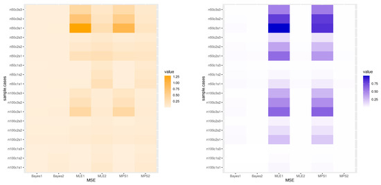
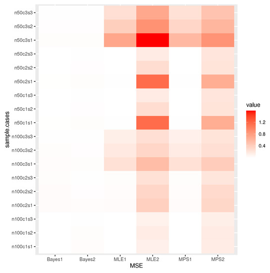
Figure 6. Heat maps of MSE results.

X-label: Bayes1 is the MSE of a for the Bayesian, Bayes2 is the MSE of $\beta$ for the Bayesian, MPS1 is the MSE of a for the MPS, MPS2 is the MSE of $\beta$ for the MPS, MLE1 is the MSE of a for the MLE, and MLE2 is the MSE of $\beta$ for the MLE.

Y-label: n50c1s1 is the MSE when $n=50$, $a=0.35$, $r=25$, and the first T value; n50c1s2 is the MSE when $n=50$$a=0.35$, $r=35$, and the second T value; n50c1s3 is the MSE when $n=50$, $a=0.35$, $r=50$, and the third T value; n50c2s1 is the MSE when $n=50$, $a=1.2$, $r=25$, and the first T value; n50c2s2 is the MSE when $n=50$, $a=1.2$, $r=35$, and the second T value; n50c2s3 is the MSE when $n=50$, $a=1.2$, $r=50$, and the third T value; n50c3s1 is the MSE when $n=50$, $a=3$, $r=25$, and the first T value; n50c3s2 is the MSE when $n=50$, $a=3$, $r=35$, and the second T value; n50c3s3 is the MSE when $n=50$, $a=3$, $r=50$, and the third T value; n100c1s1 is the MSE when $n=100$, $a=0.35$, $r=70$, and the first T value; n100c1s2 is the MSE when $n=100$, $a=0.35$, $r=85$, and the second T value; n100c1s3 is the MSE when $n=100$, $a=0.35$, $r=100$, and the third T value; n100c2s1 is the MSE when $n=100$, $a=1.2$, $r=70$, and the first T value; n100c2s2 is the MSE when $n=100$, $a=1.2$, $r=85$, and the second T value; n100c2s3 is the MSE when $n=100$, $a=1.2$, $r=100$, and the third T value; n100c3s1 is the MSE when $n=100$, $a=3$, $r=70$, and the first T value; n100c3s2 is the MSE when $n=100$, $a=3$, $r=85$, and the second T value; n100c3s3 is the MSE when $n=100$, $a=3$, $r=100$, and the third T value. The dark color indicates that the MSE value is large, while the light color indicates that the MSE value is small.

7. Application of Real Data

In this section, three actual data sets are used to demonstrate the TCP-ITL distribution’s potential. The TCP-ITL distribution is contrasted with many rival models, including the odd log-logistic modified Weibull (OLLMW) distribution by Saboor et al. [44], Kumaraswamy Weibull (KW) distribution by Cordeiro et al. [45], extended odd Weibull Lomax (EOWL) distribution by Alsuhabi et al. [46], Weibull–Lomax (WL) distribution by Tahir et al. [47], extended Weibull (EW) distribution by Peng et al. [48], modified Kies inverted Topp–Leone (MKITL) distribution by Almetwally et al. [49], inverse Weibull (IW) distribution and X-gamma Lomax (XGL) distribution by Almetwally et al. [50], generalized inverse Weibull (GIW) distribution by De Gusmao et al. [51], and gamma distribution.

For Global Reserves Natural data set I in Table 7, we obtained different comparison models in Table 8 and results of estimation methods. Table 9, Table 10 and Table 11 provide values for the Cramer–von Mises (CVM), Anderson–Darling (AD), and Kolmogorov–Smirnov (KSD) statistics, along with their P-values (PVKS), for all the models fitted based on the three real data sets. These statistics include the Akaike information criterion (AIC), correct Akaike information criterion (CAIC), Bayesian information criterion (BIC), and Hannan–Quinn. The MLE and standard errors (SE) of the parameters for the models under consideration are also included in these tables. The SE values were obtained by the square root of the diagonal of the inverse of a Hessian matrix, where we obtained the Hessian matrix by using the ’maxLik’ package. When compared to all the other models applied to each real data set in Table 9, Table 10 and Table 11, the TCP-ITL distribution has the highest P-value and the lowest KS, CvM, AD, AIC, BIC, HQIC, and CAIC values.

Table 7. The percent Global Reserves Natural Gas of the Countries (2020).

Rank	Country	% Global Reserves	Rank	country	% Global Reserves
1	Russia	19.9	23	Ukraine	0.6
2	Iran	17.1	24	Malaysia	0.5
3	Qatar	13.1	25	Uzbekistan	0.4
4	Turkmenistan	7.2	26	Oman	0.4
5	United States	6.7	27	Vietnam	0.3
6	China	4.5	28	Israel	0.3
7	Venezuela	3.3	29	Argentina	0.2
8	Saudi Arabia	3.2	30	Pakistan	0.2
9	UAE	3.2	31	Trinidad	0.2
10	Nigeria	2.9	32	Brazil	0.2
11	Iraq	1.9	33	Myanmar	0.2
12	Canada	1.3	34	United Kingdom	0.1
13	Australia	1.3	35	Thailand	0.1
14	Azerbaijan	1.3	36	Mexico	0.1
15	Algeria	1.2	37	Bangladesh	0.1
16	Kazakhstan	1.2	38	Netherlands	0.1
17	Egypt	1.1	39	Bolivia	0.1
18	Kuwait	0.9	40	Brunei	0.1
19	Norway	0.8	41	Peru	0.1
20	Libya	0.8	42	Syria	0.1
21	Indonesia	0.7	43	Yemen	0.1
22	India	0.7	44	Papua New Guinea	0.1

Table 8. MLE and Bayesian estimation for TCP-ITL based on hybrid censored samples: Data I.

			MLE				Bayesian
r	T		Estimates	SE	Lower	Upper	Estimates	SE	Lower	Upper
44	max(X)	a	1.1550	0.3181	0.5315	1.7785	3.1200	0.2646	2.9017	4.0398
		$\beta$	0.5046	0.0825	0.3428	0.6664	1.2419	0.0521	0.9838	1.3469
35	0.6	a	1.6910	0.9337	0.1390	3.5210	5.2507	0.8119	4.6740	5.7682
		$\beta$	0.5646	0.1286	0.3124	0.8167	1.1762	0.1266	0.7058	1.2751
35	1.3	a	1.7091	0.6172	0.4994	2.9188	5.1838	0.7314	4.8602	5.7866
		$\beta$	0.5720	0.1077	0.3609	0.7831	1.4081	0.1030	0.9885	1.6014
40	6	a	1.0551	0.3351	0.3982	1.7119	2.9117	0.6727	1.7629	4.3244
		$\beta$	0.4900	0.0835	0.3264	0.6535	1.1507	0.0921	0.7596	1.5817

Table 9. MLE and different measures for each model of Data set I Global Reserves Natural.

		Estimates	SE	KSD	PVKS	AIC	BIC	HQIC	CAIC	CVM	AD
TCP-ITL	a	1.1550	0.3181	0.1417	0.3401	131.9224	135.4908	132.2151	133.2457	0.1378	1.0693
	$\beta$	0.5046	0.0825
ITL	$\alpha$	2.3646	0.3565	0.2992	0.0008	153.2059	154.9901	153.3012	153.8676	0.1465	1.1182
OLLMW	$\alpha$	12.4358	8.0350	0.1371	0.3797	135.3472	142.4840	136.3729	137.9939	0.1398	1.0957
	$\beta$	0.0010	0.0021
	$\theta$	0.7124	0.0169
	$\lambda$	0.0591	0.0391
KW	$\alpha$	6.4653	3.9410	0.1779	0.1234	133.6958	140.8326	134.7214	136.3424	0.1386	1.0840
	$\beta$	0.4598	0.4665
	$\theta$	25.6596	25.0357
	$\lambda$	0.4001	0.1156
EOWL	$\alpha$	3.3258	2.0215	0.1438	0.3231	132.2461	139.3829	133.2718	134.8928	0.1389	1.0902
	$\beta$	1.0951	1.5178
	$\theta$	0.1754	0.0568
	$\lambda$	0.0098	0.0124
EW	$\alpha$	0.5880	0.0753	0.1785	0.1212	140.8229	146.1754	141.4229	142.8078	0.2236	1.5563
	$\beta$	98.5859	75.3859
	$\theta$	0.1139	0.0503
MKITL	$\alpha$	0.4394	0.0593	0.1642	0.1861	133.9317	137.5001	135.2551	134.2244	0.1640	1.2311
	$\beta$	1.4542	0.2583
IW	$\alpha$	0.7922	0.0965	0.1602	0.2087	141.9545	142.5545	147.307	143.9394	0.2396	1.6480
	$\beta$	0.3889	0.0870
GIW	$\alpha$	0.4919	0.8661	0.1602	0.2088	136.5200	141.8726	138.5050	137.1200	0.1390	1.0993
	$\beta$	0.6825	0.9034
	$\theta$	0.7918	0.0965
Gamma	$\alpha$	0.5034	0.0887	0.1980	0.0635	144.6730	148.2414	144.9657	145.9963	0.3039	2.0003
	$\beta$	0.2240	0.0618

Table 10. MLE and different measures for each model of Senegal COVID-19 data II.

		Estimates	SE	KSD	PVKS	AIC	BIC	HQIC	CAIC	CVM	AD
TCP-ITL	$\alpha$	46.4611	9.4888	0.0885	0.9507	−64.7732	−61.9053	−64.3447	−63.8383	0.0311	0.2435
	$\beta$	2.7087	0.7494
EK	$\alpha$	0.3571	0.4269	0.1094	0.8134	−63.2672	−58.9652	−62.3783	−61.8649	0.0389	0.2669
	$\beta$	6.1680	2.6239
	$\theta$	104.0626	35.8501
APK	$\alpha$	0.0237	0.0481	0.0882	0.9520	−61.4001	−57.0981	−60.5112	−59.9978	0.0371	0.3426
	$\beta$	3.0733	0.4271
	$\theta$	27.3055	20.9555
MOK	$\alpha$	13.3874	3.2429	0.11037	0.8051	−56.4469	−52.145	−55.5581	−55.0446	0.0798	0.6778
	$\beta$	1.1461	0.8567
	$\theta$	15.3077	10.0012
K	$\alpha$	2.4382	0.3335	0.1353	0.5751	−59.9538	−57.0858	−59.5252	−59.0189	0.0741	0.6409
	$\beta$	31.9917	14.6988
Beta	$\alpha$	4.7004	1.1552	0.1083	0.8225	−63.0484	−60.1804	−62.6198	−62.1135	0.0440	0.3988
	$\beta$	17.4681	4.4646
ITL	$\alpha$	30.2539	5.4338	0.1904	0.1853	−55.7185	−54.2845	−55.5805	−55.2510	0.0341	0.3048
Gamma	$\alpha$	6.1575	1.5235	0.0916	0.9358	−64.3018	−61.4338	−63.8732	−63.3669	0.0331	0.2886
	$\beta$	29.1566	7.5164

Table 11. MLE and different measures for each model of the flood level data III.

		Estimates	SE	KSD	PVKS	AIC	BIC	HQIC	CAIC	CVM	AD
TCP-ITL	a	30.4065	6.4173	0.1284	0.8964	−28.4612	−26.4698	−27.7553	−28.0725	0.0454	0.2768
	$\beta$	11.4472	5.7151
EK	$\alpha$	0.2393	0.1882	0.1508	0.7534	−26.0267	−23.0395	−24.5267	−25.4436	0.0626	0.3739
	$\beta$	4.3099	1.0001
	$\theta$	815.3741	185.8772
APK	$\alpha$	103.3454	57.3081	0.1864	0.4904	−21.2119	−18.2247	−19.7119	−20.6287	0.1384	0.8266
	$\beta$	1.7417	0.4553
	$\theta$	7.8359	2.8893
MOK	$\alpha$	0.0152	0.0347	0.1300	0.8877	−25.8470	−22.8598	−24.3470	−25.2639	0.0514	0.3292
	$\beta$	6.4466	1.2659
	$\theta$	5.3311	11.0554
K	$\alpha$	3.3787	0.6043	0.2176	0.2998	−21.9465	−19.9551	−21.2407	−21.5578	0.1673	0.9748
	$\beta$	12.0126	5.4759
Beta	$\alpha$	6.8315	2.1181	0.2063	0.3625	−24.3671	−22.3757	−23.6613	−23.9784	0.1267	0.7514
	$\beta$	9.2373	2.8915
ITL	$\alpha$	10.6952	2.3915	0.3721	0.0079	−6.4280	−5.4322	−6.2058	−6.2336	0.0699	0.4305
Gamma	$\alpha$	13.5708	4.2398	0.1726	0.5906	−26.8643	−24.8728	−26.1584	−26.4756	0.0753	0.4619
	$\beta$	32.1197	10.2224

Figure 7, Figure 8 and Figure 9 show the fit empirical, histogram, QQ-plot, and PP-plot for the TCP-ITL distribution for the COVID-19 data of the United Kingdom and Canada.

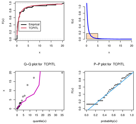
Figure 7. Fitted PDF for Global Reserves Natural data set I.

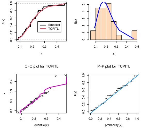
Figure 8. Fitted PDF for Senegal COVID-19 data set II.

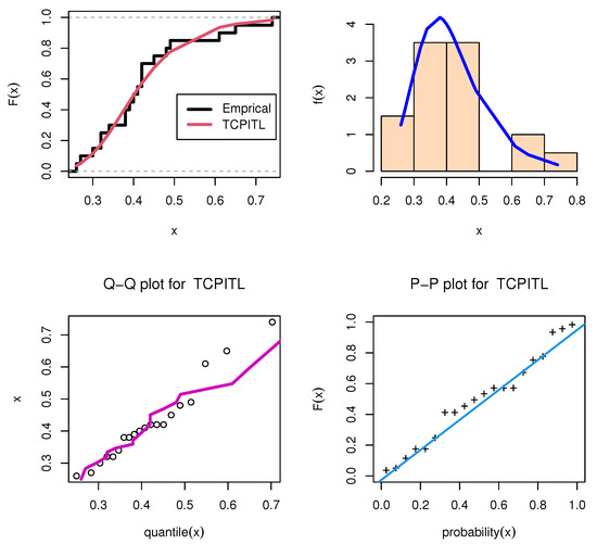
Figure 9. Fitted PDF for flood level data set III.

Table 8, Table 12, and Table 13 discuss the different estimation methods for the parameters of the TCP-ITL distribution based on the hybrid censored samples. By these results, we note the time T increases and the size r increases, and the SE decreased. The Bayesian estimation method has the smallest SE for the parameters of the TCP-ITL distribution based on the hybrid censored samples comparing the MLE. The MPS is not applicable in data I and III because we note the data sets have the same observation.

Table 12. MLE, MPS, and Bayesian estimation for parameters of TCP-ITL based on hybrid censored samples: Data II.

			MLE				MPS				Bayesian
r	T		Estimates	SE	Lower	Upper	Estimates	SE	Lower	Upper	Estimates	SE	Lower	Upper
31	1	a	46.4063	9.4815	27.8226	64.9900	46.4063	9.4815	27.8226	64.9900	22.9116	4.9305	14.0346	32.8419
		$\beta$	2.7053	0.7484	1.2384	4.1722	2.7053	0.7484	1.2384	4.1722	1.8495	0.4806	0.9842	2.7881
20	0.2	a	47.8768	14.6865	19.0912	76.6623	40.2913	13.7695	13.3030	67.2796	4.2107	2.1515	1.4998	6.9777
		$\beta$	2.7959	1.0181	0.8004	4.7913	2.2561	0.8198	0.6494	3.8628	0.7513	0.2465	0.3795	1.1235
20	0.25	a	47.1387	12.5108	22.6176	71.6599	40.8599	11.8221	17.6887	64.0311	7.9281	2.7097	3.4907	12.5283
		$\beta$	2.7611	0.9107	0.9762	4.5461	2.2833	0.7497	0.8138	3.7528	0.9641	0.2724	0.5293	1.4805
25	0.25	a	50.3660	11.6432	27.5453	73.1866	44.6581	11.0658	22.9692	66.3471	12.7954	3.3827	6.9520	19.2480
		$\beta$	2.9630	0.9138	1.1720	4.7540	2.4867	0.7619	0.9934	3.9801	1.2119	0.3141	0.6683	1.8111

Table 13. MLE and Bayesian estimation for TCP-ITL based on hybrid censored samples with different cases: Data set III.

			MLE				Bayesian
r	T		Estimates	SE	Lower	Upper	Estimates	SE	Lower	Upper
20	1	a	30.4065	6.4173	17.8286	42.9843	17.5977	2.5528	11.0885	24.5465
		$\beta$	11.4472	5.7151	0.2456	22.6487	3.4733	0.8221	1.4866	5.7411
15	0.45	a	34.8751	7.8562	19.4770	50.2733	11.8472	3.0320	6.1586	17.5158
		$\beta$	15.5375	7.9139	0.0263	33.0088	1.9487	0.8781	0.9094	3.2611
18	0.5	a	34.0657	7.3325	19.6941	48.4374	14.2534	2.9212	8.6380	20.6930
		$\beta$	14.7475	7.2701	0.4981	30.4805	2.4022	0.8691	1.0307	3.8191

For the Bayesian estimation, we discussed Figure 10, Figure 11 and Figure 12 of the MCMC results to check the convergences, and we conclude the MCMC results have convergence.

Figure 10. Trace and posterior density with normal curve for MCMC results for data I.

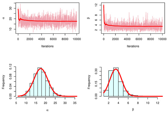
Figure 11. Trace and posterior density with normal curve for MCMC results: Data II.

Figure 12. Trace and posterior density with normal curve for MCMC results: Data III.

7.1. Data Set I

The first data set represents the percent of the Global Reserves of Natural Gas of the Countries (2020). The data set was obtained from the following electronic address: https://worldpopulationreview.com/country-rankings/natural-gas-by-country. The data set is reported in Table 7.

7.2. Data Set II

The second data set was obtained from the WHO [52], with the set of data belonging to Senegal for 31 days from 18 July 2021 to 17 August 2021 where the mortality rate received for COVID-19 is 0.1017, 0.1179, 0.1361, 0.1720, 0.1885, 0.1867, 0.1465, 0.0904, 0.2144, 0.0883, 0.2447, 0.1207, 0.1869, 0.2504, 0.3282, 0.2271, 0.2897, 0.1437, 0.4596, 0.2817, 0.2469, 0.1528, 0.2269, 0.1954, 0.4639, 0.2820, 0.1323, 0.2334, 0.2470, 0.1882, and 0.2022. The mortality rate equation is

$$\mathrm{mortality}{\mathrm{rate}}_j=\frac{\mathrm{New}{\mathrm{deaths}}_j}{\mathrm{Cumulative}{\mathrm{cases}}_i-\mathrm{Cumulative}{\mathrm{deaths}}_{(i-1)}}$$

Throughout this subsection, we apply the TCP-ITL model to a real-world data set to assess its adaptability. To compare the TCP-ITL model to the other six fitted distributions, one, two, and three parameters are employed. We compare the TCP-ITL distribution with the ITL [23], beta, Kumaraswamy (K), Marshall–Olkin–Kumaraswamy (MOK) [53], alpha power Kumaraswamy (MOK) [54], and exponentiated Kumaraswamy (EK) [55].

The parameter estimates of the MLE with the standard error (SE) and the numerical value are presented in Table 9 and Table 10. Moreover, the numerical values of the KSD and its PVKS, AIC, BIC, HQIC, and CAIC statistics for the data sets are presented in Table 9 and Table 10. From Table 9 and Table 10, the values of the KSD, AIC, BIC, HQIC, and CAIC are minimum for the TCP-ITL distribution. Thus, the TCP-ITL distribution is a better model for the data sets as compared with the other six models. Figure 7, Figure 8 and Figure 9 display the fitted PDF plots of each data set.

7.3. Data Set III

The third data set, given in Dumonceaux and Antle, includes 20 observations of the maximum flood level (in millions of cubic feet per second) for the Susquehanna River near Harrisburg, Pennsylvania [56], and Mazucheli et al. [57]. The data are as follows: 0.26, 0.27, 0.30, 0.32, 0.32, 0.34, 0.38, 0.38, 0.39, 0.40, 0.41, 0.42, 0.42, 0.42, 0.45, 0.48, 0.49, 0.61, 0.65, 0.74.

8. Concluding Remarks

In this article, the truncated Cauchy power family is combined with the inverted Topp–Leone distribution to create a new two-parameter model called the truncated Cauchy power-inverted Topp–Leone distribution. Some statistical and mathematical features of the TCP-ITL distribution are implemented, including the quantile function, moments and incomplete moments, the moment-generating function, and various types of entropy, such as the R$\acute{e}$nyi entropy, Havrda and Charvat entropy, Tsallis entropy, and Arimoto entropy (ArE). The maximum likelihood (ML), maximum product of spacing (MPSP), and Bayesian estimate approaches are investigated for complete and hybrid censored data. To test the proposed distribution’s restricted sample attributes, a simulation study is created. The majority of the time, the numerical data revealed that the Bayesian estimates were more accurate than the comparable alternative estimates. Examples from dependability, medicine, and engineering demonstrate the adaptability of the proposed approach. The potential of the TCP-ITL distribution is demonstrated in comparison with some known distributions using three real-world data sets. According to the results of the criteria measurements, the proposed distribution is the best option for the data sets under consideration.

References

- Taketomi, N.; Yamamoto, K.; Chesneau, C.; Emura, T. Parametric Distributions for Survival and Reliability Analyses, a Review and Historical Sketch. Mathematics 2022, 10, 3907. [Google Scholar] [CrossRef]
- Aldahlan, M.A.; Jamal, F.; Chesneau, C.; Elgarhy, M.; Elbatal, I. The Truncated Cauchy power family of distributions with inference and applications. Entropy 2020, 22, 346. [Google Scholar] [CrossRef]
- Alotaibi, N.; Elbatal, I.; Almetwally, E.M.; Alyami, S.A.; Al-Moisheer, A.S.; Elgarhy, M. Truncated Cauchy Power Weibull-G Class of Distributions: Bayesian and Non-Bayesian Inference Modelling for COVID-19 and Carbon Fiber Data. Mathematics 2022, 10, 1565. [Google Scholar] [CrossRef]
- Chaudhary, A.K.; Sapkota, L.P.; Kumar, V. Truncated Cauchy Powera Inverse Exponential Distribution: Theory and Applications. IOSR J. Math. 2020, 16, 12–23. [Google Scholar]
- Shrahili, M.; Elbatal, I. Truncated Cauchy power odd Fréchet family of distributions: Theory and applications. Complexity 2021, 2021, 4256945. [Google Scholar] [CrossRef]
- Almarashi, A.M. Truncated Cauchy power Lomax model and its application to biomedical data. Nanosci. Nanotechnol. Lett. 2020, 12, 16–24. [Google Scholar] [CrossRef]
- Barco, K.V.P.; Mazucheli, J.; Janeiro, V. The inverse power Lindley distribution. Commun. Stat.-Simul. Comput. 2017, 46, 6308–6323. [Google Scholar] [CrossRef]
- Abd AL-Fattah, A.M.; El-Helbawy, A.A.; Al-Dayian, G.R. Inverted Kumumaraswamy distribution: Properties and estimation. Pak. J. Stat. 2017, 33, 37–61. [Google Scholar]
- Almutiry, W. Inverted Length-Biased Exponential Model: Statistical Inference and Modelling. J. Math. 2021, 2021, 1980480. [Google Scholar] [CrossRef]
- Chiodo1, E.; Falco, P.D.; Noia, L.P.D.; Mottola, F. Inverse Log-logistic distribution for extreme wind speed modeling: Genesis, identification and Bayes estimation. AIMS Energy 2018, 6, 926–948. [Google Scholar] [CrossRef]
- Eliwa, M.S.; El-Morshedy, M.; Ibrahim, M. Inverse Gompertz distribution: Properties and different estimation methods with application to complete and censored data. Ann. Data Sci. 2019, 6, 321–339. [Google Scholar] [CrossRef]
- Sharma, V.K.; Singh, S.K.; Singh, U.; Agiwal, V. The inverse Lindley distribution: A stress-strength reliability model with application to head and neck cancer data. J. Ind. Prod. Eng. 2015, 32, 162–173. [Google Scholar] [CrossRef]
- Mahmoud, M.A.W.; Ghazal, M.G.M.; Radwan, H.M.M. Inverted generalized linear exponential distribution as a lifetime model. Appl. Math. Inf. Sci. 2017, 11, 1747–1765. [Google Scholar] [CrossRef]
- Louzada, F.; Ramos, P.L.; Nascimento, D. The Inverse Nakagami-m Distribution: A Novel Approach in Reliability. IEEE Trans. Reliab. 2018, 67, 1030–1042. [Google Scholar] [CrossRef]
- Tahir, M.H.; Cordeiro, G.M.; Ali, S.; Dey, S.; Manzoor, A. The inverted Nadarajah-Haghighi distribution: Estimation methods and applications. J. Stat. Comput. Simul. 2018, 88, 2775–2798. [Google Scholar] [CrossRef]
- Al-Kzzaz, H.S.; El-Monsef, M.M.E.A. Inverse power Maxwell distribution: Statistical properties, estimation and application. J. Appl. Stat. 2022, 49, 2287–2306. [Google Scholar] [CrossRef] [PubMed]
- Hassan, A.S.; Abd-Allah, M. On the inverse power Lomax distribution. Ann. Data Sci. 2018, 6, 259–278. [Google Scholar] [CrossRef]
- Chesneau, C.; Yousof, H.; Hamedani, G.; Ibrahim, M. The Discrete Inverse Burr Distribution with Characterizations, Properties, Applications, Bayesian and Non-Bayesian Estimations. Stat. Optim. Inf. Comput. 2022, 10, 352–371. [Google Scholar] [CrossRef]
- Hussain, T.; Ahmad, M. Discrete inverse Rayleigh distribution. Pak. J. Stat. 2014, 30, 203–222. [Google Scholar]
- Jazi, A.M.; Lai, D.C.; Alamatsaz, H.M. Inverse Weibull distribution and estimation of its parameters. Stat. Methodol. 2010, 7, 121–132. [Google Scholar] [CrossRef]
- Adetunji, A.A.; Ademuyiwa, J.A.; Adejumo, O.A. The Inverse Sushila Distribution: Properties and Application. Asian Res. J. Math. 2020, 16, 28–39. [Google Scholar] [CrossRef]
- Jordanova, P.K.; Petkova, M.P.; Stehlík, M. Inverse Log-Gamma-G processes. AIP Conf. Proc. 2017, 1895, 030003. [Google Scholar]
- Hassan, A.S.; Elgarhy, M.; Ragab, R. Statistical properties and estimation of inverted Topp-Leone distribution. J. Stat. Appl. Probab. 2020, 9, 319–331. [Google Scholar]
- Abushal, T.A.; Hassan, A.S.; El-Saeed, A.R.; Nassr, S.G. Power inverted Topp- Leone distribution in acceptance sampling plans. Comput. Mater. Contin. 2021, 67, 991–1011. [Google Scholar] [CrossRef]
- Hassan, A.S.; Almetwally, E.M.; Ibrahim, G.M. Kumaraswamy inverted Topp-Leone distribution with applications to COVID-19data. Comput. Mater. Contin. 2021, 68, 337–356. [Google Scholar]
- Ibrahim, G.M.; Hassan, A.S.; Almetwally, E.M.; Almongy, H.M. Parameter estimation of alpha power inverted Topp-Leone distribution with applications. Intell. Autom. Soft Comput. 2021, 29, 353–371. [Google Scholar] [CrossRef]
- Bantan, R.; Elsehetry, M.; Hassan, A.S.; Elgarhy, M.; Sharma, D.; Chesneau, C.; Jamal, F. A Two-Parameter Model: Properties and Estimation under Ranked Sampling. Mathematics 2021, 9, 1214. [Google Scholar] [CrossRef]
- Alizadeh, M.; Lak, F.; Rasekhi, M.; Ramires, T.G.; Yousof, H.M.; Altun, E. The odd log-logistic Topp-Leone G family of distributions: Heteroscedastic regression modelsand applications. Comput. Stat. 2018, 33, 1217–1244. [Google Scholar] [CrossRef]
- Chipepa, F.; Oluyede, B.; Peter, O.P. The Burr III-Topp-Leone-G family of distributions with applications. Heliyon 2021, 7, e06534. [Google Scholar] [CrossRef]
- MacGillivray, H.L. Skewness and asymmetry: Measures and orderings. Ann. Stat. 1986, 14, 994–1011. [Google Scholar] [CrossRef]
- Nadarajah, S.; Kotz, S. Some beta distributions. Bull. Braz. Math. Soc. 2006, 37, 103–125. [Google Scholar] [CrossRef]
- Rényi, A. On measures of entropy and information. Berkeley Symp. Math. Stat. Probab. 1961, 1961, 547–561. [Google Scholar]
- Havrda, J.; Charvat, F. Quantification method of classification processes, Concept of Structural -Entropy. Kybernetika 1967, 3, 30–35. [Google Scholar]
- Tsallis, C. The role of constraints within generalized nonextensive statistics. Physica 1998, 261, 547–561. [Google Scholar] [CrossRef]
- Arimoto, S. Information-theoretical considerations on estimation problems. Inf. Control 1971, 19, 181–194. [Google Scholar] [CrossRef]
- Balakrishnan, N.; Kundu, D. Hybrid censoring: Models, inferential results and applications. Comput. Stat. Data Anal. 2013, 57, 166–209. [Google Scholar] [CrossRef]
- Singh, S.; Tripathi, Y.M. Bayesian estimation and prediction for a hybrid censored lognormal distribution. IEEE Trans. Reliab. 2015, 65, 782–795. [Google Scholar] [CrossRef]
- Chen, M.H.; Shao, Q.M. Monte Carlo estimation of Bayesian credible and HPD intervals. J. Comput. Graph. Stat. 1999, 8, 69–92. [Google Scholar]
- Dey, S.; Singh, S.; Tripathi, Y.M.; Asgharzadeh, A. Estimation and prediction for a progressively censored generalized inverted exponential distribution. Stat. Methodol. 2016, 32, 185–202. [Google Scholar] [CrossRef]
- Henningsen, A.; Toomet, O. maxLik: A package for maximum likelihood estimation in R. Comput. Stat. 2011, 26, 443–458. [Google Scholar] [CrossRef]
- Plummer, M.; Best, N.; Cowles, K.; Vines, K. Package ‘Coda’. Available online: http://cran.r-project.org/web/packages/coda/coda.pdf (accessed on 25 January 2015).
- El-Sherpieny, E.S.A.; Almetwally, E.M.; Muhammed, H.Z. Progressive Type-II hybrid censored schemes based on maximum product spacing with application to Power Lomax distribution. Phys. A Stat. Mech. Its Appl. 2020, 553, 124251. [Google Scholar] [CrossRef]
- Singh, U.; Singh, S.K.; Singh, R.K. Product spacings as an alternative to likelihood for Bayesian inferences. J. Stat. Appl. Probab. 2014, 3, 179–188. [Google Scholar] [CrossRef]
- Saboor, A.; Alizadeh, M.; Khan, M.N.; Ghosh, I.; Cordeiro, G.M. Odd log-logistic modified Weibull distribution. Mediterr. J. Math. 2017, 14, 1–19. [Google Scholar] [CrossRef]
- Cordeiro, G.M.; Ortega, E.M.; Nadarajah, S. The Kumaraswamy Weibull distribution with application to failure data. J. Frankl. Inst. 2010, 347, 1399–1429. [Google Scholar] [CrossRef]
- Alsuhabi, H.; Alkhairy, I.; Almetwally, E.M.; Almongy, H.M.; Gemeay, A.M.; Hafez, E.H.; Sabry, M. A superior extension for the Lomax distribution with application to Covid-19 infections real data. Alex. Eng. J. 2022, 61, 11077–11090. [Google Scholar] [CrossRef]
- Tahir, M.H.; Cordeiro, G.M.; Mansoor, M.; ZUBAÄ°R, M. The Weibull-Lomax distribution: Properties and applications. Hacet. J. Math. Stat. 2015, 44, 455–474. [Google Scholar] [CrossRef]
- Peng, X.; Yan, Z. Estimation and application for a new extended Weibull distribution. Reliab. Eng. Syst. Saf. 2014, 121, 34–42. [Google Scholar] [CrossRef]
- Almetwally, E.M.; Alharbi, R.; Alnagar, D.; Hafez, E.H. A New Inverted Topp-Leone Distribution: Applications to the COVID-19 Mortality Rate in Two Different Countries. Axioms 2021, 10, 25. [Google Scholar] [CrossRef]
- Almetwally, E.M.; Kilai, M.; Aldallal, R. X-Gamma Lomax Distribution with Different Applications. J. Bus. Environ. Sci. 2022, 1, 129–140. [Google Scholar] [CrossRef]
- De Gusmao, F.R.; Ortega, E.M.; Cordeiro, G.M. The generalized inverse Weibull distribution. Stat. Pap. 2011, 52, 591–619. [Google Scholar] [CrossRef]
- WHO World Health Organization. Responding to Community Spread of COVID-19. 2020. Available online: https://www.who.int/ (accessed on 28 January 2023).
- Chakraborty, S.; Handique, L. The generalized Marshall-Olkin-Kumaraswamy-G family of distributions. J. Data Sci. 2017, 15, 391–422. [Google Scholar] [CrossRef] [PubMed]
- Ahmed, M.A. On the alpha power Kumaraswamy distribution: Properties, simulation and application. Rev. Colomb. Estad. 2020, 43, 285–313. [Google Scholar] [CrossRef]
- Lemonte, A.J.; Barreto-Souza, W.; Cordeiro, G.M. The exponentiated Kumaraswamy distribution and its log-transform. Braz. J. Probab. Stat. 2013, 27, 31–53. [Google Scholar] [CrossRef]
- Dumonceaux, R.; Antle, C.E. Discrimination between the log-normal and the Weibull distributions. Technometrics 1973, 15, 923–926. [Google Scholar] [CrossRef]
- Mazucheli, J.; Menezes, A.F.; Dey, S. Unit-Gompertz distribution with applications. Statistica 2019, 79, 25–43. [Google Scholar]
Disclaimer/Publisher’s Note: The statements, opinions and data contained in all publications are solely those of the individual author(s) and contributor(s) and not of MDPI and/or the editor(s). MDPI and/or the editor(s) disclaim responsibility for any injury to people or property resulting from any ideas, methods, instructions or products referred to in the content. |
© 2023 by the authors. Licensee MDPI, Basel, Switzerland. This article is an open access article distributed under the terms and conditions of the Creative Commons Attribution (CC BY) license (https://creativecommons.org/licenses/by/4.0/).