Article

Study of the Hypergeometric Equation via Data Driven Koopman-EDMD Theory

1
Department of Economics, National and Kapodistrian University of Athens, 1, Sofokleous Str., 10559 Athens, Greece
2
Department of Business Administration, National and Kapodistrian University of Athens, 1, Sofokleous Str., 10559 Athens, Greece
3
Lehrstuhl Wirtschafts-und Betribswissenschaften (wBw), Montanuniversität Leoben, Franz Josef Straße 18, A-8700 Leoben, Austria
*
Author to whom correspondence should be addressed.
Axioms 2023, 12(2), 134; https://doi.org/10.3390/axioms12020134
Submission received: 24 December 2022 / Revised: 22 January 2023 / Accepted: 23 January 2023 / Published: 29 January 2023
(This article belongs to the Special Issue Special Topics in Differential Equations with Applications)

Abstract

:
We consider a data-driven method, which combines Koopman operator theory with Extended Dynamic Mode Decomposition. We apply this method to the hypergeometric equation which is the Fuchsian equation with three regular singular points. The space of solutions at any of its singular points is a two-dimensional linear vector space on the field of reals when the independent variable is restricted to take values in the real axis and the unknown function is restricted to be a real-valued function of a real variable. A basis of the linear vector space of solutions is spanned by the hypergeometric function and its products with appropriate powers of the independent variable or the logarithmic function depending on the roots of the indicial equation of the hypergeometric equation. With our work, we obtain a new representation of the fundamental solutions of the hypergeometric equation and relate them to the spectral analysis of the finite approximation of the Koopman operator associated with the hypergeometric equation. We expect that the usefulness of our results will come more to the fore when we extend our study into the complex domain.
MSC:
37P99; 34A45; 34M99

1. Introduction

The study of complex nonlinear dynamical systems appears in many disciplines, such as physics, engineering, biology, social sciences, etc. The high degree of complexity of such systems makes their analysis quite a challenge. From this point of view, data-driven mathematical methods might be of high importance. These methods aspire to exploit measurement data, which form a relatively small subset of the original state space. However, they might describe the evolution of the original system, even if its dynamics are complicated or unknown. In recent years, it seems that advances in numerical techniques and the broader availability of data have brought data-driven methods to the forefront of scientific research. For example, one such technique might as well be Koopman operator theory in connection with Dynamic Mode Decomposition (DMD), and especially with Extended Dynamic Mode Decomposition (EDMD).
Firstly, in the Koopman operator framework (initiated in [1], see also [2,3]), the central objects are complex-valued functions defined on the state space (these functions are called observables of the systems). The Koopman operator describes the evolution of the observables according to the evolution of the system. This approach enables us to “lift” the dynamical system from its original state space to new spaces spanned by observables.
The main advantage is that the Koopman operator is linear. Hence, powerful methods from operator theory, such as spectral analysis, can be applied. The Koopman operator might be quite useful especially when we study in high-dimensional and strongly non-linear systems. In these cases, the phase space is quite large and its dynamics are so complicated that very little can be concluded about its corresponding geometrical properties. Applications of this approach range from, among others, fluid dynamics (see [4,5]), energy modeling in buildings (see [6]), oceanography (see [7]) and molecular kinetics (see [8]).
Despite its advantages, the Koopman operator converts a finite-dimensional system to an infinite-dimensional linear system. In other words, we “pay” in dimensions, in order to gain “linearity”. Being infinite-dimensional, the Koopman operator cannot be calculated while its spectral properties are difficult to explore. In practice, this amounts to a simplification only when one can handle the operator numerically. Consequently, the need for numerical methods that generate finite dimensional approximations of the Koopman operator is emerging.
In this direction, dynamic mode decomposition (DMD) (see [9,10]) and its generalization, the extended-DMD (EDMD) have been proven very efficient. Since these methods depend on data and rely only on least square regression, they are very easy to implement.
The EDMD method algorithm starts by choosing a finite set of observables, which is called a dictionary. Then, we approximate the Koopman operator as a linear map on the span of this finite set. Note that the finite-dimensional linear map which emerges in such a case is numerically tractable. Furthermore, its spectral properties can approximate those of the Koopman operator (see [11]).
Critical to the success of the EDMD algorithm is the appropriate choice of the dictionary. The choice of a suitable dictionary significantly impacts the approximation quality of the spectral properties of the system (see [11,12,13]). However, in many practical applications, it is often not so easy to make such a selection without some prior information on the dynamics of the system.
The Koopman operator-EDMD algorithm has been applied to several ODEs and PDEs. For example, see [14] for an application to Burgers’ equation and the nonlinear Scrödinger equation. Moreover, see [15] for an application to Kuramoto–Sivashinsky PDE. In this paper, we demonstrate the use of the Koopman-EDMD method when applied to the hypergeometric equation. The effectiveness of our approach is based on the choice of the appropriate dictionary.
The hypergeometric equation is a linear second-order homogeneous differential equation that falls into the Fuchsian class and has three regular singular points at 0 , 1 , and . In this paper, we restrict the independent variable to be real and the dependent variable to be a real−valued function of a real variable. At each singular point, there is a fundamental set of two solutions that span the two-dimensional linear vector solution space.
Summarizing our discussion, the innovation and contribution of this paper are summarized as follows: We address the trajectory approximation of a hypergeometric equation via EDMD methods. The EDMD method gives rise to a linear system on an enhanced state space that can approximate a given trajectory. Having data of a given trajectory in a finite horizon allows us to construct a discrete linear system of dimension n > m , where m is the dimension of the state space of the original nonlinear system. We demonstrate the approximation of a single trajectory of a hypergeometric equation via EDMD methods. In particular, we solve a hypergeometric equation in the vicinity of 0, which is one of its singular points, by using the Koopman-EDMD theory. Finally, we show that we can improve the approximation of the solution of a hypergeometric equation in the vicinity of 0, by using successive trajectory reconstruction via Koopman-EDMD theory with moving horizon.
The EDMD method is data-driven. Consequently, depending on a suitable choice, the method can be applied to any dynamical system for which probably the dynamical law is unknown and data, in the form of time series, can be collected for some of its trajectories in the state space. Moreover, our approach can be used for any nonlinear dynamical system with known dynamics. However, in such a case a linearization of the dynamics via the EDMD method may be required in order, for example, to study the control theory of this linearized system; the control theory of linear systems is much better understood than the control theory of nonlinear systems.
The rest of the paper is organized as follows. In Section 2, we briefly present some basic facts about the Koopman operator theory and EDMD method. In Section 3, we give an example of a hypergeometric equation and its exact solution via hypergeometric series. In Section 4, we solve the hypergeometric equation in the interval ( 0.9 , 0.001 ) via Koopman-EDMD theory. In Section 5, we solve the hypergeometric equation in the interval ( 0.2 , 1 ) via Koopman-EDMD theory. In Section 6, we present a successive trajectory reconstruction via Koopman-EDMD theory with a moving horizon. Finally, Section 7 contains our conclusions about this paper.

2. Koopman Operator and EDMD

Koopman operator theory has been extensively used in the analysis, prediction, and control of nonlinear dynamical systems. To define this class of operators, we start with a continuous dynamical system M , f , where M is the state space (usually a manifold in R n ) and f is the evolution map. The system is described by the differential equation x ˙ = f ( x ) . We also denote by Φ t ( x 0 ) the flow map, which is defined as the state of the system in time t when the initial condition is x 0 .
In the literature of Koopman operators, complex-valued functions g : M C defined on M are called observables of the system ( M , f ) . We now consider a function space F of observables which is closed under composition with the flow map. This means that g Φ t belongs to F whenever g F . (In many applications, F is the space L 2 ( M ) of complex valued square integrable functions on M . However, other function spaces can also be considered.) Then, for any t 0 , the operator K t : F F is defined by K t ( g ) = g Φ t . The term Koopman operator usually refers to the whole class of operators, i.e., K = ( K t ) t 0 . The linearity of composition implies that K t is a linear operator for any t 0 .
In a similar way, the Koopman operator can be defined for discrete dynamical systems, which, in some sense, are more natural. Indeed, in many practical applications, the differential equations that describe the evolution of the system are completely unknown and we have only measurement data that are provided in discrete time. So, let us assume that we are given a discrete system, x k + 1 = f ( x k ) , where x k belongs to the state space M . The Koopman operator is defined as the composition of any observable with the evolution map f. Thus, K : F F is given by K ( g ) = g f , for any g F . (Again, F is a function space of observables closed under composition with f).
By its definition, the Koopman operator updates every observable according to the evolution of the dynamical system. A new system ( F , K ) is defined which is a global linearization of the original system ( M , f ) (i.e., it does not hold only to the area of some attractor or fixed point). Furthermore, many properties of ( M , f ) can be related to the eigenstructure of K (see [16]). Consequently, one can utilize tools from functional analysis and operator theory in order to study the system ( M , f ) even if this is a nonlinear one.
The main advantage of the Koopman operator is its linearity. However, it is infinite-dimensional and, except in some cases, we can calculate neither the operator nor its eigenstructure. In order to address the problems that infinite dimensionality poses, we have to look for finite-dimensional linear approximations of the Koopman operator. Towards this direction, the Dynamic Mode Decomposition (DMD) and, mainly, its generalization the Extended Dynamic Mode Decomposition (EDMD) have been proven very successful.

Extended Dynamic Mode Decomposition (EDMD)

We next give a brief description of the EDMD algorithm. The first step is to fix a set of observables { g 1 , g 2 , , g p } , which is usually called a dictionary. In the case of DMD (Dynamic Mode Decomposition), we use only the observables g i ( x ) = x i , for i = 1 , 2 , , n . On the contrary, in EDMD any observable can be chosen. In this way, we construct an augmented state space and; hence, EDMD gives better approximation properties than DMD. The augmented state space is denoted by M ¯ and its elements are denoted by y = [ g 1 ( x ) , , g p ( x ) ] T .
The second step involves data collection. To this end, we consider a trajectory of the original system with some initial condition x 0 and some finite time horizon T. Then, we collect sampling points at a fixed time interval Δ T (although, uniform sampling is not mandatory and one can apply other sampling methods). Therefore, we consider n 0 = T Δ T points in this trajectory, which are denoted by ( x s ) s = 0 n 0 . These points generate data ( y s ) s = 0 n 0 in the augmented space M ¯ . Finally, the data are organized in data matrices as follows
Y [ 0 , n 0 1 ] = y 0 , y 1 , , y n 0 1 and Y [ 1 , n 0 ] = y 1 , y 2 , , y n 0 .
The last step is to obtain a p × p matrix A (using, for instance, least square regression methods) such that Y [ 1 , n 0 ] A Y [ 0 , n 0 1 ] . Therefore,
A = argmin A ˜ R p × p Y [ 1 , n 0 ] A ˜ Y [ 0 , n 0 1 ] ,
where · is some matrix norm.
The procedure described above can be applied to several trajectories. Hence, we may fix k trajectories and, following the previous steps, we obtain data matrices Y j [ 0 , n 0 1 ] and Y j [ 01 , n 0 ] for every j = 1 , 2 , , k . In this case, the matrix A is chosen such that
A = argmin A ˜ R p × p j = 1 k Y j [ 1 , n 0 ] A ˜ Y j [ 0 , n 0 1 ] .
Consequently, A is a best-fit matrix that relates the two data matrices in every trajectory. The matrix A generates a finite-dimensional linear system that advances spatial measurements from one time to the next and it provides approximations to the Koopman operator and to the original nonlinear system.
One of the main advantages of EDMD is that it is a purely data-driven method. Therefore, there is actually no restriction to its applicability and it can be utilized even if the dynamics of the system are completely unknown. However, the success of this method depends on the a priori chosen dictionary. In many problems, the most difficult part is to choose a dictionary that will give good approximations. There is no generic algorithm for this problem, however, some recent studies use artificial intelligence methods in order to “train” the dictionary (see [15,17]).

3. An Example of Hypergeometric Equation and Its Exact Solution via Hypergeometric Series

We consider the hypergeometric equation
t ( t 1 ) d 2 x d t 2 + ( 2 t 1 ) d x d t + x = 0 ,
with initial conditions t = 0.9 , x ( 0.9 ) = 0.1 , d x d t t = 0.9 = 1 . The solution of the complexification of (1) with the aforementioned initial conditions is given by
( 16.9355 + 11.3861 i ) L e g e n d r e P 1 2 i i + 3 , 1 + 2 t + ( 0.00524496 0.649963 i ) L e g e n d r e Q 1 2 i i + 3 , 1 + 2 t
where L e g e n d r e P denotes the Legendre function of the first kind and L e g e n d r e Q denotes the Legendre function of the second kind. Figure 1 depicts the plot of the real part of the solution (2). We observe that the solution has vertical asymptotes at the singular points t = 0 , t = 1 of (1). In the next section, we numerically integrate (1) and reproduce the solution of (1) in the connected interval t ( 0.9 , 0.001 ) .

4. Solving the Hypergeometric Equation in the Interval ( 0 . 9 , 0 . 001 ) via Koopman-EDMD Theory

We numerically integrate
t ( t 1 ) d 2 x d t 2 + ( 2 t 1 ) d x d t + x = 0 ,
with initial conditions t = 0.9 , x ( 0.9 ) = 0.1 , d x d t t = 0.9 = 1 in the interval t ( 0.9 , 0.001 ) . Subsequently, we sample the trajectory with a time step Δ t = 0.01 .  Figure 2 depicts the graph of the sampled points showing the asymptotic trend at t = 0 .
We then apply EDMD interpolation, as described in Section 2, using a dictionary of 4 observables, namely x , 1 x , t x , t x . The EDMD algorithm provides the following 4 × 4 transition matrix
1.08228 0.401294 0.145089 0.131762 0.00886136 1.01576 0.00552547 0.00574604 0.0075471 0.35145 0.628826 0.252387 0.0127506 0.332983 0.354283 1.23706
The above matrix has 4 eigenvalues, two of which are real and the other two are complex numbers. In particular, the eigenvalues are
1.11249 , 0.987529 + 0.00693293 i , 0.987529 0.00693293 i , 0.876376 .
Figure 3 shows the position of these eigenvalues in the complex plane.
The above matrix gives rise to a (finite-dimensional) linear dynamical system, whose trajectory (for the specific initial conditions) approximates the real trajectory. The comparison between the two trajectories approximated (orange line) and real data (blue line) is shown in Figure 4. Despite the low dimensions of this approximation, the Koopman-EDMD curve approximates well the given data away from the singularity at t = 0 and fails to do so near t = 0 . It is possible to considerably improve the approximation by augmenting the dictionary both quantitatively and qualitatively.

Improving the Trajectory Approximation via Koopman-EDMD Theory

We follow on by augmenting the dictionary and repeating the trajectory approximation via EDMD. The dictionary that produces the best results and at the same time the dimension of the augmented space is kept comparatively low (equal to 5) is given by x , 1 x , t x , t x , x t 15 . The comparison between the real trajectory and the approximation provided by the EDMD algorithm is presented in Figure 5. We notice that the approximation is significantly improved.
The matrix provided by the EDMD algorithm is now given by
1.08292 0.387515 0.126814 0.119021 1.67268 0.00887233 1.01553 0.00583752 0.0059636 0.0285622 0.0162179 0.537512 0.382055 0.424438 22.5875 0.0213778 0.518112 0.599816 1.40825 22.4742 0.0000448427 0.00187752 0.00186914 0.00143044 0.799134
This matrix has two complex eigenvalues and three real eigenvalues, namely
1.11308 , 0.986969 + 0.00680815 i , 0.986969 0.00680815 i , 0.901002 , 0.699867 .
Their positions in the complex plane are depicted in Figure 6.

5. Solving the Hypergeometric Equation in the Interval ( 0 . 2 , 1 ) via Koopman-EDMD Theory

Figure 7 shows the plot of the real part of the solution (2) in the interval [ 0 , 1 ] (this is also depicted in Figure 1).
This solution has vertical asymptotes at the singular points of (1), that is, at t = 0 , t = 1 . We are going to numerically integrate (1) and reproduce the solution of (1) by Koopmman-EDMD theory in the connected interval ( 0.2 , 1 ) .
We approximate this solution in the interval ( 0.2 , 1 ) by using the EDMD basis x , 1 x , t x , t x , x t 0.1 . The five-dimensional discrete linear system obtained this way approximates satisfactorily the trajectory in the interval ( 0.2 , 1 ) as shown in Figure 8.
The EDMD matrix is given by
8.03736 3.0825 5.23571 6.45347 10.0906 7.37378 4.18128 5.39554 6.58341 10.5197 0.0144556 0.00620308 0.978249 0.00396585 0.0199957 0.00137726 0.00686054 0.020928 0.975436 0.00765612 7.15414 3.10723 5.294 6.46348 9.23167
which has the following eigenvalues
1.10972 , 0.984838 + 0.0194333 i , 0.984838 0.0194333 i , 0.959174 , 0.902077 .

6. Successive Trajectory Reconstruction via Koopman-EDMD Theory with Moving Horizon

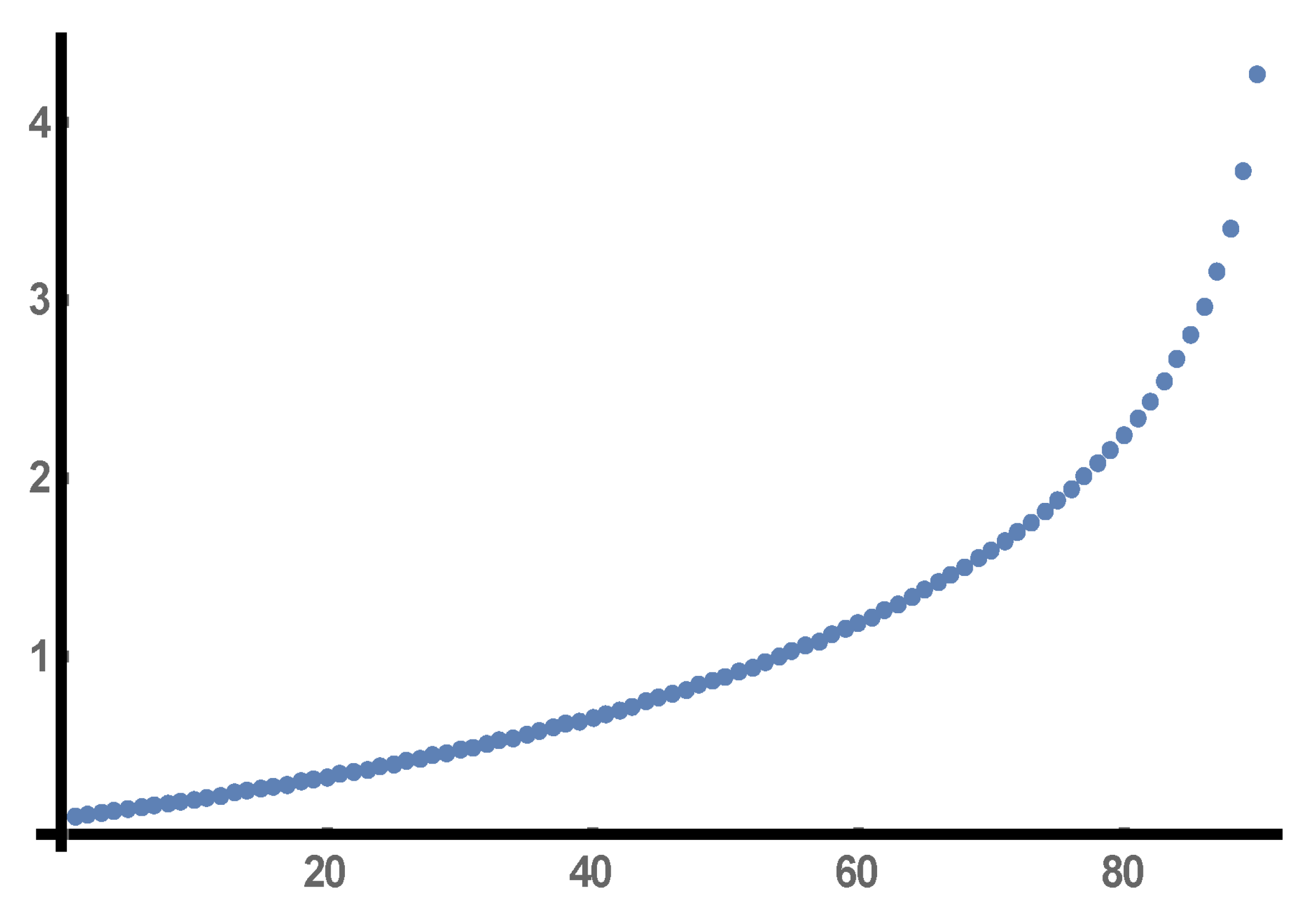
We apply EDMD trajectory reconstruction for t ( 0 , 1 ) of the real part of the solution (2) of the differential Equation (1) whose graph is depicted in Figure 1.
We consider a four-dimensional EDMD basis consisting of x , 1 x , t x , t x , and we cover the interval [ 0.05 , 0.95 ] with 14 overlapping windows each of which contains 41 sample points of the hypergeometric solution. We then apply 14 EDMD computations for the 14 moving windows and produce 14 approximating trajectories as well as an equal number of EDMD matrices. The errors between these approximations compared to the real data and measured by the l 2 (Euclidean) norm for all 14 horizons are depicted in Figure 9 and, thus, the approximation is considered very satisfactory.
The 14 successive approximating trajectories to the hypergeometric solution (2) of Equation (1) which cover the interval [ 0.05 , 0.95 ] are given by
P x A k n x o k = a 1 k λ 1 k n + a 2 k λ 2 k n + a 3 k λ ¯ 2 k n + a 4 k λ 4 k n ,
where k = 0 , , 14 enumerates the 14 EDMD computations for the 14 moving windows and the resulting approximating trajectories, n = 0 , , 40 enumerates the 41 sample points at each window, x o k is a 4 × 1 vector of initial conditions for the basis functions x , 1 x , t x , t x , for each one of the EDMD computations, A k is the 4 × 4 EDMD matrix for each of the moving windows, P x is the 1 × 4 projection matrix to the one-dimensional space spanned by x, λ ¯ 2 k is the complex conjugate of λ 2 k , λ 1 k , λ 2 k , λ ¯ 2 k , λ 4 k are the eigenvalues of the matrices A k , and a 1 k , a 2 k , a 3 k , a 4 k 
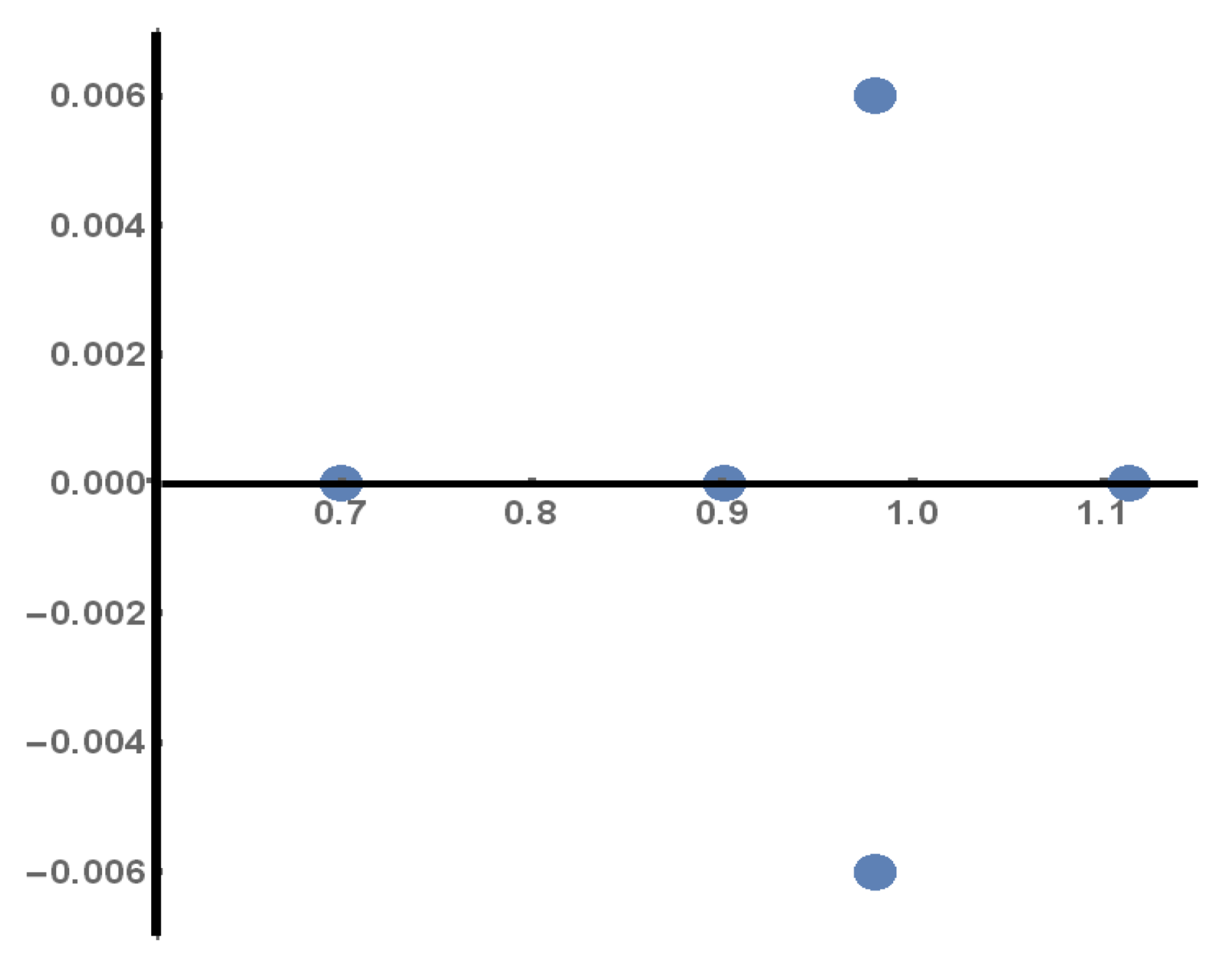
are real coefficients. In the three diagrams of Figure 10, we depict from left to right the real eigenvalue λ 1 k , which is the largest, versus k, the modulus | λ 2 k | = | λ ¯ 2 k | of the complex conjugate eigenvalues λ 2 k , λ ¯ 2 k , which are the intermediate, versus k, and the real eigenvalue λ 4 k , which is the smallest, versus k. It becomes evident from the diagrams that the largest real eigenvalue λ 1 k dominates in the approximating trajectory at the vicinity of the t = 1 asymptote.

7. Conclusions

The hypergeometric equation is a linear second-order homogeneous differential equation that falls into the Fuchsian class and has three regular singular points at 0 , 1 , and . The solution space of the hypergeometric equation is two-dimensional with basis vectors hypergeometric series. We present an alternative data-driven method in order to solve the hypergeometric equation. This method, the Koopman-EDMD method, whose popularity has increased over the last years, does not use power series but it uses instead a basis of functions, remarkably 4 or 5. The Koopman-EDMD method is data-driven and we use it in order to approximate a trajectory of the hypergeometric equation at hand in the vicinity of 0 which is one of its singular points. Having data of a given trajectory in a finite horizon allows us to construct with the Koopman-EDMD theory a discrete linear system of dimension n > m , where m = 2 is the dimension of the state space of the hypergeometric equation. In our approach, we have n = 4 or n = 5 depending on how accurate we want to be the approximation to the real trajectory of the hypergeometric equation. It is noteworthy that we approximate with great accuracy the real trajectory of the hypergeometric equation by a small increase in the number of dimensions of the state space (2 is increased only to 4 or 5 in the Koopman-EDMD theory. The Koopman-EDMD theory can be used as an alternative theory in order to study the solution space of both ordinary differential equations and of partial differential equations. Our results are amenable for application and generalization to these other cases of differential equations as well.

Author Contributions

All authors contributed equally. All authors have read and agreed to the published version of the manuscript.

Funding

This research received no external funding.

Data Availability Statement

No new data were created or analyzed in this study. Data sharing is not applicable to this article.

Conflicts of Interest

The authors declare no conflict of interest.

References

  1. Koopman, B.O. Hamiltonian systems and transformation in Hilbert space. Proc. Natl. Acad. Sci. USA 1931, 17, 315–318. [Google Scholar] [CrossRef] [PubMed] [Green Version]
  2. Brunton, S.; Kutz, N. Data-Driven Science and Engineering: Machine Learning, Dynamical Systems, and Control; Cambridge Univerisy Press: Cambridge, UK, 2019. [Google Scholar]
  3. Mauroy, A.; Mezić, I.; Susuki, Y. (Eds.) The Koopman Operator in Systems and Control; 358 Lecture Notes in Control and Information Sciences; Springer: Berlin/Heidelberg, Germany, 2020; p. 358. [Google Scholar]
  4. Mezić, I. Analysis of fluid flows via spectral properties of the koopman operator. Annu. Fluid Mech. 2013, 45, 357–378. [Google Scholar] [CrossRef] [Green Version]
  5. Sharma, A.S.; Mezić, I.; McKeon, B.J. Correspondence between koopman mode decomposition, resolvent mode decomposition, and invariant solutions of the navier-stokes equations. Phys. Rev. Fluids 2016, 1, 032402. [Google Scholar] [CrossRef]
  6. Georgescu, M.; Mezić, I. Building energy modeling: A systematic approach to zoning and model reduction using koopman mode analysis. Energy Build. 2015, 86, 794–802. [Google Scholar] [CrossRef]
  7. Giannakis, D.; Slawinska, J.; Zhao, Z. Spatiotemporal feature extraction with datadriven Koopman operators. J. Mach. Learn. Res. Proc. 2015, 44, 103–115. [Google Scholar]
  8. Wu, H.; Nüske, F.; Paul, F.; Klus, S.; Koltai, P.; Noć, F. Variational koopman models: Slow collective variables and molecular kinetics from short off-equilibrium simulations. J. Chem. Phys. 2017, 146, 154104. [Google Scholar] [CrossRef] [PubMed] [Green Version]
  9. Rowley, C.W.; Mezić, I.; Bagheri, S.; Schlatter, P.; Henningson, D.S. Spectral analysis of nonlinear flows. J. Fluid Mech. 2009, 641, 115–127. [Google Scholar] [CrossRef] [Green Version]
  10. Schmid, P.J. Dynamic mode decomposition of numerical and experimental data. J. Fluid Mech. 2010, 656, 5–28. [Google Scholar] [CrossRef] [Green Version]
  11. Korda, M.; Mezić, I. On convergence of extended dynamic mode decomposition to the Koopman operator. J. Nonlinear Sci. 2018, 28, 687–710. [Google Scholar] [CrossRef] [Green Version]
  12. Williams, M.O.; Kevrekidis, I.G.; Rowley, C.W. A DataDriven Approximation of the Koopman Operator: Extending Dynamic Mode Decomposition. J. Nonlinear Sci. 2015, 25, 1307–1346. [Google Scholar] [CrossRef] [Green Version]
  13. Williams, M.O.; Rowley, C.W.; Kevrekidis, I.G. A kernel approach to data-driven koopman spectral analysis. arXiv 2014, arXiv:1411.2260. [Google Scholar]
  14. Nathan Kutz, J.; Proctor, J.L.; Brunton, S.L. Applied Koopman Theory for Partial Differential Equations and Data-Driven Modeling of Spatio-Temporal Systems. Complexity 2018, 2018, 6010634. [Google Scholar] [CrossRef]
  15. Li, Q.; Dietrich, F.; Bollt, E.M.; Kevrekidis, I.G. Extended dynamic mode decomposition with dictionary learning: A data-driven adaptive spectral decomposition of the Koopman operator. Chaos 2017, 27, 103111. [Google Scholar] [CrossRef] [PubMed]
  16. Mezić, I. Spectral properties of dynamical systems, model reduction and decompositions. Nonlinear Dyn. 2005, 41, 309–325. [Google Scholar] [CrossRef]
  17. Folkestad, C.; Pastor, D.; Mezic, I.; Mohr, R.; Fonoberova, M.; Burdick, J. Extended Dynamic Mode Decomposition with Learned Koopman Eigenfunctions for Prediction and Control. In Proceedings of the 2020 American Control Conference (ACC), Denver, CO, USA, 1–3 July 2020; pp. 3906–3913. [Google Scholar] [CrossRef]
Figure 1. Graph of the real part of the solution (2).
Axioms 12 00134 g001
Figure 2. The graph of the sampled points of the hypergeometric Equation (1).
Axioms 12 00134 g002
Figure 3. The eigenvalues of the EDMD transition matrix depicted in the complex plane.
Axioms 12 00134 g003
Figure 4. The real data (blue line) and the approximate trajectory (orange line).
Axioms 12 00134 g004
Figure 5. Comparison between the real trajectory (blue line) and the trajectory (orange line) given by the EDMD algorithm with a dictionary of five observables.
Axioms 12 00134 g005
Figure 6. Eigenvalues of the 5 × 5 matrix produced by the EDMD methodology.
Axioms 12 00134 g006
Figure 7. Graph of the real part of the solution (2) in the interval [ 0 , 1 ] .
Axioms 12 00134 g007
Figure 8. Comparison between approximated (orange line) and real data (blue line) in the interval ( 0.2 , 1 ) .
Axioms 12 00134 g008
Figure 9. Errors between the 14 EDMD approximating trajectories and real data measured by the l 2 (Euclidean) norm.
Axioms 12 00134 g009
Figure 10. The graph of (a) the largest real eigenvalue; (b) the modulus of the complex conjugate eigenvalues; (c) the smallest real eigenvalue versus k.
Axioms 12 00134 g010
Disclaimer/Publisher’s Note: The statements, opinions and data contained in all publications are solely those of the individual author(s) and contributor(s) and not of MDPI and/or the editor(s). MDPI and/or the editor(s) disclaim responsibility for any injury to people or property resulting from any ideas, methods, instructions or products referred to in the content.

