Two Reliable Computational Techniques for Solving the MRLW Equation

Abstract

In this paper, a numerical solution of the modified regularized long wave (MRLW) equation is obtained using the Sinc-collocation method. This approach approximates the space dimension of the solution with a cardinal expansion of Sinc functions. First, discretizing the time derivative of the MRLW equation by a classic finite difference formula, while the space derivatives are approximated by a $\theta —$weighted scheme. For comparison purposes, we also find a soliton solution using the Adomian decomposition method (ADM). The Sinc-collocation method was were found to be more accurate and efficient than the ADM schemes. Furthermore, we show that the number of solitons generated can be approximated using the Maxwellian initial condition. The proposed methods’ results, analytical solutions, and numerical methods are compared. Finally, a variety of graphical representations for the obtained solutions makes the dynamics of the MRLW equation visible and provides the mathematical foundation for physical and engineering applications.

1. Introduction

Partial differential equations, especially non-linear ones, are used in the study of many natural phenomena that often arise in the physical sciences and engineering applications. For nonlinear equations, there is a difficulty, if not an impossibility, in finding exact solutions to the equation, and researchers often resort to finding a solution with approximate methods. Here, we will use two different schemes to solve the modified equation for the long wave known as MRLW equation (see, [1,2,3]).

$$\frac{\partial u}{\partial t}+\frac{\partial u}{\partial x}+ϵu^p\frac{\partial u}{\partial x}-\mu \frac{\partial }{\partial t}\left(\frac{{\partial }^{2}u}{\partial x^2}\right)=0$$

(1)

With the following boundary and initial conditions

$$u(a,t)={\alpha }_1\left(t\right),u(b,t)={\alpha }_2\left(t\right)$$

(2)

$$u(x,0)=f\left(x\right),x\in [a,b]\subset \mathrm{I}\mathrm{R}.$$

(3)

where $ϵ$ and $\mu$ in Equation (1) are positive constants that describe the undular bore’s behavior, and p is a positive integer greater than or equal to 1, while the function $f\left(x\right)$ is a localized disturbance inside the interval $[a,b]$ subject to physical boundary conditions $u\to \infty$ as $x\to \mp \infty$. The functions that appeared on both sides in Equation (2) are also continuous. Equation (1), which we will abbreviate with MRLW, was originally a mathematical model to describe a physical phenomenon with weak scattering waves, and in another application it describes the movement of transverse waves in shallow water. There are many previous studies that dealt with the use of numerical methods to find approximate solutions to the equation under consideration, the MRLW equation. In the paper [4], the collocation method was used to find an approximate solution to the MRLW equation. The method relied mainly on the use of the Sinc function as a basis. The B-splines finite element method of order 3 was used in [5] to solve the MRLW equation numerically, the numerical results proved the accuracy of the used method. In [6], two different bases are used to solve numerically the MRLW equation, in which the finite difference method is used along the time derivatives, while the delta-shaped basis was used to discretize the space direction. It should be noted here that there are many previous studies in which the Sinc method was used or those that dealt with approximate solutions to the equation under study, among which we mention [7,8,9]. Recently published papers in [10,11,12,13,14] dealt with the use of different methods to find numerical solutions to various forms of the generalized RLW equation. For more knowledge, there are other previous studies that discussed the same ideas presented in this paper, but in different ways, such as [1,15,16].

The Sinc methodology is one of the most powerful tools for solving various types of equations that model various physical phenomena. This method is used to solve integral equations, partial differential equations, and integro-differential equations. The most important motive of this research work is the use of the Sinc method because the convergence of the approximate solution is of exponential type. For some positive constants $c,h$ the Sinc method yields an iterative scheme with an error of order $\mathcal{O}(exp(-c/h)$, which is much faster than other traditional methods.

The main objective of this paper is to find an approximate solution to the MRLW equation in (1)–(3), where the basis of the Sinc function on the variable x will be used, while we will use the regular finite difference method when talking about the time variable t. Moreover, the Adomian decomposition method will be used for comparison purposes.

The main idea of using the Sinc function is that in the process of replacing the partial derivatives that appeared in (1), in terms of the variable x, with the corresponding formulas that have been proven in both references Stenger [17] and by Lund [18], followed by the use of the Sinc quadrature formula for integration with some simple manipulations, we end up with a discrete system of the general form $Ax=b$ that can be solved iteratively via the use of iterative techniques, such as Newton’s method. What encourages us to use the Sinc function is its ease of use, and most importantly, the fast exponential convergence property when using the Sinc function as a basis. For the purpose of comparing the solution that will be obtained by the Sinc methodology, we will use the Adomian analysis method, the so-called Adomian decomposition method (ADM) [19,20], to find another solution in an approximate (not numerical) way. The ADM method was created and developed at the beginning of the 1980s of the last century, and it has proven its worth when used in various nonlinear, ordinary and partial differential equations. There are many previous studies that dealt with finding a solution to linear or nonlinear, ordinary or partial differential equations, via the use of ADM, see for example [21,22,23]. Those equations represented a mathematical model in several fields, including physics, chemistry, biology, engineering in its various forms and medical sciences. The ADM is summarized as finding a solution in the form of a convergent series, and often we need a number that does not exceed the number of fingers on one hand to obtain an appropriate solution, knowing that in previous studies there is sufficient and convincing evidence for the convergence of the method to an accurate solution.

The general structure of this paper can be reviewed as follows: In Section 2, we present the main concepts of the Sinc function and all the theories we need in writing the solution to Equation (1). As for Section 3, we will discuss the formulation of the solution using the Sinc-collocation method, while Section 4 is limited to talking about the stability of the calculated solution. Section 5 is where we will present the alternative method, which is ADM. The effectiveness of the solution presented by the two methods in this paper is discussed in Section 6 by taking two different values of the constant p. The credibility of the methods used will be shown by presenting the numerical results in the form of tables and graphs, and finally, a summary of what happened with some recommendations in Section 7.

2. Sinc-Collocation

The Sinc function method has proven its effectiveness in finding approximate solutions to many problems with physical and engineering applications. The Sinc function is considered to be some kind of wavelet that has been used effectively in recent years to find solutions to many problems. Here, we will review some important characteristics that we will use to formulate the solution using the basis of the Sinc function. These are discussed in [17,18]. It is known that the Sinc function is defined in the domain of all real numbers as follows

$$\mathrm{sinc}\left(x\right)=\frac{sin\left(\pi x\right)}{\pi x},x\in \mathrm{I}\mathrm{R}.$$

(4)

We will use the Sinc function for the purposes of interpolation, over the defined interval of the question under consideration. To do so, we first divide the interval into sub-intervals, each of which is h, and then redefine the Sinc function as follows:

$$S_j\left(x\right)=\mathrm{sinc}\left(\frac{x-jh}{h}\right),j=0,\mp 1,\mp 2,\dots$$

(5)

In order to use the formula in Equation (5) as a basis, then for every continuous function $f\left(x\right)$, we define an infinite series, known as Whittaker cardinal function, denoted by $C(f,h)$, and defined to be

$$C(f,h)\left(x\right)=\sum _{j=-\infty }^{\infty }f\left(ih\right)S_j\left(x\right).$$

We know very well that we cannot deal with an infinite series, so we will deal with a finite series, ensuring its convergence within certain conditions, which we will impose on the function to be approximated, so N can be a positive integer, we define the series of $2N+1$ terms as

$$C_N(f,h)\left(x\right)=\sum _{j=-N}^N{f}_j{S}_j\left(x\right).$$

(6)

We use the above series to approximate the $nth$ derivative of the function f, and is given by the relationship

$$f^{\left(n\right)}\approx \sum _{j=-N}^{N}f\left(jh\right)\frac{d^n}{d{x}^n}\left[S_j\left(x\right)\right].$$

(7)

In fact, we need the derivatives of the Sinc function computed at the nodes on which the period was divided, and in this paper we need the first and second derivatives only, so that we can write the solution in the form of a system of linear equations, as we will see in detail later. We also require derivatives of composite Sinc functions evaluated at the nodes. The expressions are required for the present discussion, so the following convenient notation will be needed [17].

$${\delta }_{j-k}^{\left(0\right)}=\left[S_j\left(x\right)\right]{|}_{x=x_k}=\left\{\begin{array}{c}1,j=k\hfill \\ \\ 0,j\ne k\hfill \end{array}\right.$$

(8)

$${\delta }_{j-k}^{\left(1\right)}=\frac{d}{dx}\left[S_j\left(x\right)\right]{|}_{x=x_k}=\left\{\begin{array}{c}0,j=k\hfill \\ \\ \frac{{(-1)}^{jk}}{h(k-j)},j\ne k\hfill \end{array}\right.$$

(9)

$${\delta }_{j-k}^{\left(2\right)}=\frac{d^2}{d{x}^2}\left[S_j\left(x\right)\right]{|}_{x=x_k}=\left\{\begin{array}{c}\frac{-{\pi }^2}{3},j=k\hfill \\ \\ \frac{-2{(-1)}^{k-j}}{{(k-j)}^2},j\ne k.\hfill \end{array}\right.$$

(10)

where the points $x_k$ appeared above, they are all those points that have been divided into the period and are called collocation points, and they will be used in the approximation process. So, we need to use a finite series that starts from the integer $-N$ and ends with the number N, but there must be a constraint or conditions that the function f, to be approximated, must fulfill or its derivatives. The next definition provides us with a property called exponentially decaying that the function must achieve for this purpose.

Definition 1.

We define a domain ${\mathcal{D}}_d$, in the form of an infinite strip of width $2d,d>0$, as

$${\mathcal{D}}_d=\{z\in \mathrm{I}\mathrm{C}:z=x+iy,|y|<d\le \pi /2\}.$$

When $0<ϵ<1$, we define the rectangular domain ${\mathcal{D}}_d\left(ϵ\right)$ by

$${\mathcal{D}}_d\left(ϵ\right)=\{z\in \mathrm{I}\mathrm{C}:z=x+iy,|x|<1/ϵ,|y|<d(1-ϵ)\}.$$

(11)

In the region ${\mathcal{D}}_d$, we define the Hardy space, denoted by $\mathcal{B}\left({\mathcal{D}}_d\right)$, to be the set of all functions f that satisfy the following boundedness condition.

$$\underset{ϵ\to 0}{lim}{\int }_{\partial {\mathcal{D}}_d\left(ϵ\right)}\left|f\left(z\right)\right|\left|dz\right|<\infty .$$

(12)

There are a lot of characteristics related to the family $\mathcal{B}\left({\mathcal{D}}_d\right)$ mentioned in [17]. Below we write a theorem that we will need when talking about the convergence of the Sinc method.

Theorem 1.

([17]). For the positive constants $\alpha ,\beta$ and d, suppose the following conditions hold true

 1. 

f belongs to the class $\mathcal{B}\left({\mathcal{D}}_d\right)$.

 2. 

the function f satisfy the decaying condition $\left|f\right(x\left)\right|\le \alpha exp(-\beta |x\left|\right),$ valid for all real-valued of x. We conclude that

$$sup|f^{\left(n\right)}\left(x\right)-\sum _{j=N}^N{f}_j{S}_j^{\left(n\right)}\left(x\right)|\le C_1{N}^{(n+1)/2}exp\left(-\sqrt{\pi d\beta N}\right)$$

for some constant $c_1$, where $h=\sqrt{\pi d/\left(\beta N\right)}.$

It can be summarized what the previous theorem stipulated as follows, if the analytic function f fulfills the vanishing condition, then we can use the Sinc function to approximate f and its $nth$-derivatives $f^{\left(n\right)}$, so that the error in the approximation is of the exponential type, which is considered to be one of the fastest types of convergence. Thus, in order for us to find an approximate solution to Equation (1), there must be a hypothesis that the initial condition belongs to the family $\mathcal{B}\left({\mathcal{D}}_d\right)$. Now, we will define some matrices that we will need to describe the solution as a discrete system.

Define three Toeplitz matrices, each of size $m\times m,(m=2N+1)$, as $I_m^{\left(q\right)}=\left[{\delta }_{j-k}^{\left(q\right)}\right],$ for values of $q=0,1,2,$ which means the matrix whose $jkth$ entry is given by ${\delta }_{j-k}^{\left(q\right)},q=0,1,2.$ The diagonal matrix $\mathcal{D}\left(g\right)$ is defined to be $\mathcal{D}\left(g\right)=\mathrm{diag}[g\left(x_{-N}\right),\cdots ,g\left(x_N\right)].$ It is known that the matrix $I^{\left(2\right)}$ is symmetric, and $I^{\left(1\right)}$ is skew-symmetric, i.e., $I_{jk}^{\left(1\right)}=-I_{kj}^{\left(1\right)}$ and they take the form

$$I_m^{\left(2\right)}=\left(\begin{array}{cccc}\frac{-{\pi }^2}{3}& 2& ⋮& \frac{{(-1)}^{m-1}}{m-1}\\ 2& .& .& .\\ ⋮& .& .& ⋮\\ \frac{{(-1)}^{m-1}}{m-1}& ⋮& 2& \frac{-{\pi }^2}{3}\end{array}\right),\mathrm{and}{I}_m^{\left(1\right)}=\left(\begin{array}{cccc}0& -1& \cdots & \frac{{(-1)}^{m-1}}{m-1}\\ 1& 0& & ⋮\\ ⋮& & & ⋮\\ \frac{{(-1)}^{m-1}}{m-1}& \cdots & 1& 0\end{array}\right)$$

(13)

It is noted that $I^{\left(0\right)}$ is the identity matrix. Because these matrices will appear in the final discrete solution, and for the purpose of demonstrating the stability property of the solution, it is necessary to find some bounds for the eigenvalues, as stated in [17]. If ${\left\{i{\lambda }_j^{\left(1\right)}\right\}}_{j=-N}^N$ indicate to be the eigenvalues of the matrix $I^{\left(1\right)}$, then $-\pi \le {\lambda }_{-N}^{\left(1\right)}\le \cdots \le {\lambda }_N^{\left(1\right)}\le \pi .$ Similarly, ${\left\{i{\lambda }_j^{\left(2\right)}\right\}}_{j=-N}^N$ indicate to be the eigenvalues of the matrix $I^{\left(2\right)}$, then $-{\pi }^2\le {\lambda }_{-N}^{\left(2\right)}\le \cdots \le {\lambda }_N^{\left(2\right)}\le {\pi }^2$.

3. Setting Up the Scheme

To accomplish the goal of finding an approximate solution for the Equation (1), using Sinc-collocation, without losing anything of importance, but for reasons related to facilitating the calculations, we will discuss the solution by the Sinc methodology when $p=2$ only. We discretize the time derivatives that appeared on the left side and the last term in Equation (1) via the use of the regular finite-difference scheme, secondly, we apply $\theta —$metric $(0\le \theta \le 1)$ scheme to the x derivatives evaluated at two time levels n and $n+1$, so we obtain

$$\begin{array}{c}\left(\frac{u^{(n+1)}-u^{\left(n\right)}}{\delta t}\right)+\theta \left[{\left(\frac{\partial u}{\partial x}\right)}^{(n+1)}+ϵ{\left(u\right)}^{(n+1)}{\left(\frac{\partial u}{\partial x}\right)}^{(n+1)}\right]+(1-\theta )\left[{\left(\frac{\partial u}{\partial x}\right)}^{\left(n\right)}+ϵ{\left(u\right)}^{\left(n\right)}{\left(\frac{\partial u}{\partial x}\right)}^{\left(n\right)}\right]\\ \\ -\frac{\mu }{\delta t}\left[{\left(\frac{{\partial }^{2}u}{\partial x^2}\right)}^{(n+1)}-{\left(\frac{{\partial }^{2}u}{\partial x^2}\right)}^{\left(n\right)}\right]=0,\end{array}$$

(14)

where the notation $u^{\left(n\right)}$ is to represent the value of the solution at time level n, i.e., $u^{\left(n\right)}=u(x,t^{\left(n\right)})$, and for the time step size $\delta t$, we denote $t^{\left(n\right)}=t^{(n-1)}+\delta t$. Before going into the process of writing the solution, it is necessary to convert the non-linear term in Equation (14) into a linear quantity and the conversion process is achieved through the use of Taylor expansion, as follows:

$${\left(u^2\right)}^{(n+1)}{\left(\frac{\partial u}{\partial x}\right)}^{(n+1)}\approx {\left(u^{\left(n\right)}\right)}^2{\left(\frac{\partial u}{\partial x}\right)}^{(n+1)}+2u^{\left(n\right)}{\left(\frac{\partial u}{\partial x}\right)}^{\left(n\right)}{u}^{(n+1)}-2{\left(u^{\left(n\right)}\right)}^2{\left(\frac{\partial u}{\partial x}\right)}^{\left(n\right)}$$

(15)

From Equations (14) and (15), we arrive at

$$\begin{array}{c}{u}^{(n+1)}+\delta t\theta \left[{\left(\frac{\partial u}{\partial x}\right)}^{(n+1)}+ϵ\left\{{\left(u^{\left(n\right)}\right)}^2{\left(\frac{\partial u}{\partial x}\right)}^{(n+1)}+2u^{\left(n\right)}{\left(\frac{\partial u}{\partial x}\right)}^{\left(n\right)}{u}^{(n+1)}\right\}\right]-\mu {\left(\frac{{\partial }^{2}u}{\partial x^2}\right)}^{(n+1)}\\ \\ =u^{\left(n\right)}+\delta t\left[ϵ(3\theta -1){\left(u^{\left(n\right)}\right)}^2{\left(\frac{\partial u}{\partial x}\right)}^{\left(n\right)}-(1-\theta ){\left(\frac{\partial u}{\partial x}\right)}^{\left(n\right)}\right]-\mu {\left(\frac{{\partial }^{2}u}{\partial x^2}\right)}^{\left(n\right)}\end{array}$$

(16)

where $u^{\left(n\right)}$ represent the $nth$ iteration in the obtained approximate solution. Next, we use the Sinc-collocation method along the space variable, for that we discretize the interval $[a,b]$ as follows: For the positive integer $N>2$, take the step-size $h=\frac{(b-a)}{N-1}$, then points of interpolation are

$$x_0=a,x_N=b,x_i=\frac{ih}{N},i=1,2,\dots ,N-1.$$

(17)

To find a solution for Equation (14), using Sinc basis, we plug in,

$$u(x,t_n)\equiv u^n\left(x\right)=\sum _{j=1}^N{u}_j^n{S}_j\left(x\right),$$

(18)

where the basis Sinc functions are given by

$$S_j\left(x\right)=\mathrm{sinc}\left(\frac{x-(j-1)h-a}{h}\right).$$

(19)

The constants $u_j$ in Equation (18) are to be determined. Hence, for each collocation point $x_i$ in (17), Equation (18) can be written as

$$u^n\left(x_i\right)=\sum _{j=1}^N{u}_j^n{S}_j\left(x_i\right),i=1,\dots ,N.$$

(20)

Replacing Equation (20) into Equation (16), the approximation evaluated at those nodes inside the interval is given by

$$\begin{array}{c}\sum _{j=1}^N{u}_j^{n+1}{S}_j^{\left(0\right)}\left(x_i\right)+\delta t\theta [\left(\sum _{j=1}^N{u}_j^{n+1}{S}_j^{\left(1\right)}\left(x_i\right)\right)+ϵ\{{\left(\sum _{j=1}^N{u}_j^n{S}_j\left(x_i\right)\right)}^2\left(\sum _{j=1}^N{u}_j^{n+1}{S}_j^{\left(1\right)}\left(x_i\right)\right)\\ \\ +2\sum _{j=1}^N{u}_j^n{S}_j\left(x_i\right)\left(\sum _{j=1}^N{u}_j^n{S}_j^{\left(1\right)}\left(x_i\right)\right)\sum _{j=1}^N{u}_j^{n+1}{S}_j\left(x_i\right)\left\}\right]-\mu \left(\sum _{j=1}^N{u}_j^{n+1}{S}_j^{\left(2\right)}\left(x_i\right)\right)\\ \\ =\sum _{j=1}^N{u}_j^n{S}_j\left(x_i\right)+\delta t[ϵ(3\theta -1){\left(\sum _{j=1}^N{u}_j^n{S}_j\left(x_i\right)\right)}^2\left(\sum _{j=1}^N{u}_j^n{S}_j^{\left(1\right)}\left(x_i\right)\right)\\ \\ -(1-\theta )\left(\sum _{j=1}^N{u}_j^n{S}_j^{\left(1\right)}\left(x_i\right)\right)]-\mu \left(\sum _{j=1}^N{u}_j^n{S}_j^{\left(2\right)}\left(x_i\right)\right).\end{array}$$

(21)

The above Equation (21) is used for all interior points $x=x_i,i=2,\dots ,N-1$. The boundary conditions are given by Equation (2) for the boundary points $x_1$ and $x_N$ can be formulated as

$$\sum _{j=1}^N{u}_j^{n+1}{S}_j\left(x_i\right)={\alpha }_1\left(t^{n+1}\right),\sum _{j=1}^N{u}_j^{n+1}{S}_j\left(x_i\right)={\alpha }_2\left(t^{n+1}\right).$$

(22)

In order to write the solution as stated in the previous two equations, and in the form of a system of matrices, we redefine the following matrices and vectors:

$$U^n={[u_1^n,u_2^n,\dots ,n_N^n]}^T,I^{\left(0\right)}=(S_j\left(x_i\right),I^{\left(1\right)}=(S_j^{\prime }\left(x_i\right),I^{\left(2\right)}=(S_j^{″}\left(x_i\right),i,j=1,\dots ,N.$$

(23)

Therefore, in matrix form, Equation (21) becomes as

$$\begin{array}{c}\left[I^{\left(0\right)}-\mu I^{\left(2\right)}+\theta \delta t\left\{I^{\left(1\right)}+ϵ\left({\left(u^{\left(n\right)}\right)}^2★I^{\left(1\right)}+2\left(u^{\left(n\right)}\circ u_x^{\left(n\right)}\right)★I^{\left(0\right)}\right)\right\}\right]u^{n+1}\hfill \\ \\ =\left[I^{\left(0\right)}-\mu I^{\left(2\right)}+\delta t\left\{ϵ(3\theta -1){\left(u^{\left(n\right)}\right)}^2★I^{\left(2\right)}-(1-\theta )I^{\left(2\right)}\right\}\right]u^n+F^{n+1}.\hfill \end{array}$$

(24)

where the multiplication of the $ith$ component of the vector $u^{\left(n\right)}$ by every element of the $ith$ row of the matrix $I^{\left(q\right)},q=0,1,2$ is denoted by the symbolic notations ★, that has been used above. While the symbol ∘ is to denote the Hadamard matrix multiplication. The discrete system in Equation (24) represents a system of $N+1$ equations in $N+1$ unknowns, which can be written in a more compact form as

$$M{u}^{n+1}=R$$

(25)

where

$$M=[A_d+A_b-\mu C+\theta \delta t\left\{B+ϵ(E+D)\right\}]$$

$$R=[A_d-\mu C+\delta t\{ϵ(3\theta -1)E-(1-\theta )B\}]u^n+F^{n+1},$$

in which the matrices $A_d,A_d,B$ and C each of size $N\times N$ and can be written as

$$A_d=[I_{ij}^{\left(0\right)},i=2,\dots ,N-1;j=1,\dots ,N,otherwise0],A_b=[I_{ij}^{\left(0\right)},i=1,N;j=1,\dots ,N,otherwise0]$$

$$B=[I_{ij}^{\left(1\right)},i=2,\dots ,N-1;j=1,\dots ,N,otherwise0],C=[I_{ij}^{\left(2\right)},i=2,\dots ,N-1;j=1,\dots ,N,otherwise0].$$

Moreover, $u_x^n=B{u}^n,D=2u^n★u_x^n★D_d,E={\left(u^n\right)}^2★B$, and $F^{n+1}={[{\alpha }_1\left(t^{n+1}\right),0,...,{\alpha }_2\left(t^{n+1}\right)]}^T.$ The approximate solution can be found from Equation (25) at any point in the interval $[a,b]$ at each time level, which can be solved by any iterative techniques. It should be noted that a previous study for a system of partial differential equations using the same method, (Sinc-collocation ) was published by the first author in [24]. For the purposes of facilitating the computing process, we offer the following algorithm, which summarizes what was stated in this section.

Algorithm Stages

We follow the following steps to write the program:

• Select collocation points inside the interval $[a,b]$.
• Select the parameters $\delta t$ and $\theta$.
• Setup the initial solution $u^{\left(0\right)}$, then use Equation (24).
• Evaluate the matrix M and the vector R in Equation (25).
• The approximate solution $u^{(n+1)}$ at the successive time level is obtained.
• If $n\delta t<T$ stop, otherwise go to step 4.

4. Stability Analysis

Here, we study briefly and in an analytical way the stability of the solution by the Sinc method for the MRLW equation. Imitation of what was performed in [4,25], if $\mathbf{U}$ represent the exact solution, while $\tilde{\mathbf{U}},$ is taken to be the numerical solution of the MRLW equation in (1). If we define the error ${\epsilon }_u^n=\mathbf{U}-\tilde{\mathbf{U}}$.

Then, the error ${\epsilon }_u^{n+1}$ can be written as

$${\epsilon }_u^{n+1}={\mathbf{U}}^{\mathbf{n}+\mathbf{1}}-{\tilde{\mathbf{U}}}^{\mathbf{n}+\mathbf{1}}=I^{\left(0\right)}{A_d}^{-1}{A}_b{\epsilon }_u^n$$

(26)

For the stability of the method, we need ${\epsilon }_u^n\to 0$, provided n is large enough. We may conclude that the scheme is stable in a numerical sense, if $\rho \left(I^{\left(0\right)}{A_d}^{-1}{A}_b\right)<1$, where the notation $\rho (.)$ represents the spectral radius. Upon passing simple calculations, it is easy to verify stability if the following two conditions are fulfilled

$$\left|\frac{1+\alpha \delta t\theta {\lambda }_3+6\alpha \delta t\theta [{\lambda }_{1N}+{\lambda }_{2N}]}{1-\alpha (1-\theta )\delta t{\lambda }_3-6\alpha (1-\theta )\delta t{\lambda }_{1N}+6\alpha \delta t\theta {\lambda }_{1N}+2\mu \delta t{\lambda }_{1N}}\right|<1$$

(27)

and

$$\left|\frac{1+\beta \delta t\theta {\lambda }_3}{1-\beta (1-\theta )\delta t{\lambda }_3-3\beta \delta t{\lambda }_{1N}}\right|<1$$

(28)

where we have used the numbers 1, ${\lambda }_1,{\lambda }_3,{\lambda }_{1N},{\lambda }_{2N}$ being eigenvalues of the matrices $I^{\left(0\right)},I^{\left(1\right)},I^{\left(3\right)},{\mathbf{U}}^n\ast I^{\left(1\right)},{\mathbf{U}}^n\ast I^{\left(0\right)}$, respectively. We use some known facts about the upper bounds for the matrices $I^{\left(1\right)},I^{\left(2\right)}$, together with the fact that ${\lambda }_1=i\left|{\lambda }_1\right|$, ${\lambda }_3=i\left|{\lambda }_3\right|$, and ${\lambda }_{1N},{\lambda }_{2N}$ are complex, after algebraic manipulation (see, [4,25]), the condition (27) must hold for all eigenvalues of the respective matrices, for the method to be stable, and for $1/2\le \theta <1$ is a necessary condition for stability, but not sufficient.

5. Adomian Decomposition Method

Our goal in this section is to introduce the performance of the second scheme, namely, the Adomian decomposition method (ADM) [19,20], and give a detailed description to setup a solution for the MRLW equation [26]. The ADM is a technique to find solutions for differential equations (partial, ordinary), linear and nonlinear, homogeneous and nonhomogeneous. First, we look at the problem under consideration in general, so any nonlinear partial differential equation can be written as

$${\mathbf{L}}_{t}u(x,t)={\mathbf{L}}_{x}u(x,t)+R\left(u(x,t)\right)+F\left(u(x,t)\right)+g(x,t)$$

(29)

where the operator ${\mathbf{L}}_x$ is to represent the highest order derivative with respect to the variable x, ${\mathbf{L}}_t$ represent the time operator, $R\left(u\right(x,t\left)\right)$ contains the remaining linear terms of lower derivatives in x, $F\left(u\right(x,t\left)\right)$ is an analytic nonlinear term, and $g(x,t)$ is the forcing inhomogeneous term. Applying the inverse operator ${\mathbf{L}}_t^{-1}$ to Equation (29), we arrive at

$$u(x,t)=u(x,0)+{\mathbf{L}}_t^{-1}\left\{{\mathbf{L}}_{x}u(x,t)+R\left(u(x,t)\right)+F\left(u(x,t)\right)+g(x,t)\right\}$$

(30)

For the use of ADM, we express the solution $u(x,t)$ of (30) by the decomposition series

$$u(x,t)=\sum _{n=0}^{\infty }{u}_n(x,t)$$

(31)

while we express the nonlinear term $F\left(u\right(x,t\left)\right)$ with an infinite sum of polynomials given by

$$F\left(u(x,t)\right)=\sum _{n=0}^{\infty }{A}_n(u_0,u_1,\dots ,u_n),$$

(32)

where the terms $u_n(x,t)$ are calculated recurrently so that the zeroth term $u_0(x,t)$ is chosen from those terms arises from the initial condition, or from the source term. Then, followed by finding the first term $u_1(x,t)$, which depends on the zeroth term, followed by finding the second term, which also depends on the first term, and so on until we reach the $nth$ component. As for calculating Adomian polynomials $A_n$, there is a general formula written by Adomian [19,20,27], and another in a famous paper for Wazwaz [27], here we present the Adomian’s formula

$$A_n=\frac{1}{n!}\frac{d^n}{d{\lambda }^n}{\left[F\left(\sum _{i=0}^n{\lambda }^i{u}_i\right)\right]}_{\lambda =0},n\ge 0.$$

The substitution of (31) and (32) into (30) yields

$$\sum _{n=0}^{\infty }{u}_n(x,t)=u(x,0)+{\mathbf{L}}_t^{-1}\left\{{\mathbf{L}}_x\sum _{n=0}^{\infty }{u}_n(x,t)+R\left(\sum _{n=0}^{\infty }{u}_n(x,t)\right)+\left(\sum _{n=0}^{\infty }{A}_n(x,t)\right)+g(x,t)\right\}.$$

(33)

As mentioned above, the components are computed in a recursive manner as

$$\begin{array}{c}{u}_0(x,t)=u(x,0)+{\mathbf{L}}_t^{-1}\left[g(x,t)\right],\hfill \\ \\ u_{k+1}(x,t)={\mathbf{L}}_t^{-1}\left[{\mathbf{L}}_x\left(u_k(x,t)\right)+R\left(u_k(x,t)\right)+\left(A_k(x,t)\right)\right],k\ge 0.\hfill \end{array}$$

(34)

Looking at the above relationships, we can say that all terms depend largely on the zeroth term, so it is desirable that the zeroth term contain the least possible number of terms. If the series converges in a suitable way, then we see that

$$u_A(x,t)=\underset{M\to \infty }{lim}\sum _{n=0}^M{u}_n(x,t)$$

(35)

where M is the number of terms that we found. Previous studies showed the convergence of the solution series presented in the Equation (35), see for example [28,29]. In order to understand more about the above explanation and presentation of the ADM method, we present in the next subsection the method applied to the equation under consideration.

Analysis of ADM

We rewrite Equation (1) in an operator form as (see, [30])

$$L_{t}u=-u_x-ϵN\left(u\right)+\mu L_{xx}\left(u_t\right)$$

(36)

with the initial condition $u(x,0)=f\left(x\right)$, where the linear operators are defined by $L_t(.)=\frac{\partial }{\partial t}(.)$ and $L_{xx}(.)=\frac{{\partial }^2}{\partial x^2}(.)$. While the term $N\left(u\right)$ represents the non-linear term $u^p{u}_x$. To start, we operate on both sides of Equation (36) with the inverse of $L_t$, denoted by $L_t^{-1}(.)={\int }_0^t.dt$ yields

$$u(x,t)=u(x,0)-L_t^{-1}\left(u_x\right)-ϵL_t^{-1}\left(N\left(u\right)\right)+\mu L_t^{-1}\left(L_{xx}\left(u_t\right)\right).$$

(37)

Assume the solution $u(x,t)$ can be represented as an infinite sum of components of the form:

$$u(x,t)=\sum _{n=0}^{\infty }{u}_n(x,t).$$

While the nonlinear operator $N\left(u\right)$ can be expressed as

$$N\left(u\right)=u^p{u}_x={\left(\frac{u^{p+1}}{p+1}\right)}_x=\sum _{n=0}^{\infty }{A}_n(u_0,u_1,\dots ,u_n).$$

In our case, as the nonlinear part in the PDE is $N\left(u\right)$, then Adomian polynomials $A_n$ can be evaluated by a formula set by Adomian

$$A_n=\frac{1}{n!}\frac{d^n}{d{\lambda }^n}\left[N\left(\sum _{i=0}^{\infty }{\lambda }^i{u}_i\right)\right]{|}_{\lambda =0}.$$

In the next, we just state the first three Adomian polynomials as:

$$A_0={\left(\frac{u_0^{p+1}}{p+1}\right)}_x,A_1={\left(u_0^p{u}_1\right)}_x,A_2={\left(p{u}_0^{p-1}\frac{u_1^2}{2!}+u_0^p{u}_2\right)}_x,$$

$$A_3={\left((p-1)p{u}_0^{p-2}\frac{u_1^3}{3!}+p{u}_0^{p-1}{u}_1{u}_2+u_0^p{u}_3\right)}_x$$

and so on. In the same way, additional polynomials can be calculated. Now, Equation (37) reduces to

$$\begin{array}{c}\sum _{n=0}^{\infty }{u}_n(x,t)=u(x,0)-L_t^{-1}\left(\sum _{n=0}^{\infty }{u}_{nx}(x,t)\right)-ϵL_t^{-1}\left(\sum _{n=0}^{\infty }{A}_n(u_0,u_1,\dots ,u_n)\right)\\ \\ +\mu L_t^{-1}\left(L_{xx}\left(\sum _{n=0}^{\infty }{u}_{nt}(x,t)\right)\right),\end{array}$$

(38)

Now, set $n=0$ into the left-hand-side to identify the zero component to be $u_0(x,t)=u(x,0)$, and for $n\ge 1$ we obtain the subsequent components as

$$u_{n+1}(x,t)=-L_t^{-1}{\left(u_n\right)}_x-ϵL_t^{-1}\left(A_n\right)+\mu L_t^{-1}\left(L_{xx}{\left(u_n\right)}_t\right),n\ge 1.$$

Then, we see that the approximate solution is given by

$$u_A(x,t)=\underset{M\to \infty }{lim}\sum _{n=0}^M{u}_n(x,t)$$

(39)

where M is the number of terms that we found.

6. Numerical Experiments and Results

This section provides numerical solutions to the MRLW equation for three standard problems: solitary wave motion and the development of the Maxwellian initial condition into solitary waves. In order to be able to determine the accuracy and effectiveness of the method, we will deal with specific values of the constants that appeared in Equation (1), and here if the value of $ϵ=6,\mu =1$ and $p=2$, then for these values, the exact solution to Equation (1) is known and this allows us to know the exact error, and so we discuss the effectiveness of the proposed schemes in this paper.

Example 1.

Let us examine the problem

$$\frac{\partial u}{\partial t}+\frac{\partial u}{\partial x}+6u^2\frac{\partial u}{\partial x}-\frac{\partial }{\partial t}\left(\frac{{\partial }^{2}u}{\partial x^2}\right)=0$$

(40)

with boundary conditions $u\to 0$, as $x\to \mp \infty$, and the initial condition

$$u(x,0)=\sqrt{c}sech\left[\sqrt{\frac{c}{\mu (c+1)}}\left(x+x_0\right)\right],$$

(41)

here, the constants $c,x_0$ are free. The exact solution is given by [31]

$$u(x,t)=\sqrt{c}sech\left[\sqrt{\frac{c}{\mu (c+1)}}\left(x-(c+1)t+x_0\right)\right].$$

(42)

Equation (40) has three polynomial invariants that are related to mass, momentum and energy and is given by [32],

$$I_1={\int }_a^{b}u(x,t)dx,I_2={\int }_a^b(u^2(x,t)+\mu u_x^2(x,t))dx,I_3={\int }_a^b(u^4(x,t)-6\mu u_x^2(x,t))dx.$$

(43)

The invariants $I_1,I_2,I_3$ are considered to be an excellent tool to measure the success of the numerical solution, especially for cases where we do not know the exact solution to the problem. The quantities $I_1,I_2$ and $I_3$ are applied to measure the conservation properties of the collocation scheme. The integrals in (43) are approximated by sums to obtain numerical values of invariants in Equation (43) at the finite domain $[a,b]$ as follows:

$$I_1\simeq h\sum _{j=0}^N{u}_j^{\left(n\right)},I_2\simeq h\sum _{j=0}^N\left({\left(u_j^{\left(n\right)}\right)}^2+\mu {\left({\left(u^{\prime }\right)}_j^{\left(n\right)}\right)}^2\right),I_3\simeq h\sum _{j=0}^N\left({\left(u_j^{\left(n\right)}\right)}^4-\mu {\left({\left(u^{\prime }\right)}_j^{\left(n\right)}\right)}^2\right)$$

(44)

The computations associated with the example were performed using Mathematica. The accuracy of ADM is demonstrated for the absolute errors $|u(x,t)-u_A(x,t)|$. We compute the quantities $I_1,I_2$ and $I_3$ to ensure the conservation laws in using ADM as an approximate tool for MRLW. In the computational work, we take $c=1,\mu =1,ϵ=6$, and the simulation is performed up to $t=1,n=8$. Table 1 shows the difference between the exact and the ADM solution $u_A(x,t)$. From Table 1, we can read that results show a high degree of accuracy and efficiency of the ADM. Since the changes of invariants $I_1,I_2$ and $I_3$ are less than ${10}^{-4},{10}^{-5}$ and ${10}^{-6}$, respectively, our scheme is sensibly conservative, and our results are recorded in Table 1.

Table 1. Invariants for MRLW equation using ADM when $c=0.01$ and $0\le x\le 60$. We used $xEy$ to denote $x\times {10}^y$.

t	${\mathit{I}}_1$	${\mathit{I}}_2$	${\mathit{I}}_3$	$|\mathit{u}(\mathit{x},\mathit{t})-{\mathit{u}}_{\mathit{A}}(\mathit{x},\mathit{t})|$
0	$3.082210$	$0.201518$	$0.000678011$	$6.28820\mathrm{E}-08$
$0.1$	$3.082210$	$0.201518$	$0.000678015$	$1.22231\mathrm{E}-08$
$0.2$	$3.082208$	$0.201518$	$0.000678019$	$6.32709\mathrm{E}-07$
$0.3$	$3.082205$	$0.201517$	$0.000678021$	$2.72210\mathrm{E}-07$
$0.4$	$3.082202$	$0.201515$	$0.000678025$	$3.77219\mathrm{E}-06$
$0.5$	$3.082201$	$0.201515$	$0.000678027$	$1.70010\mathrm{E}-06$
$0.6$	$3.082201$	$0.201512$	$0.000678029$	$6.00899\mathrm{E}-05$
$0.7$	$3.082200$	$0.201512$	$0.000678029$	$3.91129\mathrm{E}-05$
$0.8$	$3.082196$	$0.201510$	$0.000678032$	$5.59981\mathrm{E}-04$
$0.9$	$3.082190$	$0.201510$	$0.000678036$	$3.72210\mathrm{E}-04$
$1.0$	$3.082184$	$0.201506$	$0.000678039$	$1.00287\mathrm{E}-04$

In our computational work for the Sinc-collocation method, we take $\alpha =1.5,\mu =0.1,ϵ=6$, and two different values of the time step sizes $\delta t=0.1$ and $\delta t=0.05$, where our interval is taken to be $[-30,30]$ and, the $N=160$ for the points in Equation (17). We use the $L_2,L_{\infty }$ [4,33], defined below to measure the accuracy of our schemes

$$L_2=\Vert \mathbf{u}-\tilde{\mathbf{u}}{\Vert }_2=\sqrt{h\sum _{j=1}^N{|{\mathbf{u}}_j-{\tilde{\mathbf{u}}}_j|}^2},L_{\infty }=\Vert \mathbf{u}-\tilde{\mathbf{u}}{\Vert }_{\infty }=\underset{1\le j\le N}{max}|{\mathbf{u}}_j-{\tilde{\mathbf{u}}}_j|$$

where $\mathbf{u}$ and $\tilde{\mathbf{u}}$ represent the exact and approximate solutions, respectively, and h is the minimum distance between any two points in Equation (18). We calculate the convergence with respect to time t, according to the following relationship [4,33]

$$\mathrm{Order}=\frac{{log}_{10}\left(\Vert u_{exact}-u_{\delta t_j}\Vert /\Vert u_{exact}-u_{\delta t_{j+1}}\Vert \right)}{{log}_{10}(\delta t_j/\delta t_{j+1})},$$

where the numerical solution with step size $\delta t_j$ is denoted by $u_{\delta t_j}$. The numerical solutions are shown in Table 2 and Table 3, where invariant and error norms for solitary waves are presented. Looking at the last column in Table 2, we see that the order of convergence is almost 2. The numerical solutions that are shown in Figure 1, Figure 2 and Figure 3. Figure 1 shows the plot of a single soliton solution for different values of time T using the Sinc-collocation method. These solutions are the bell-shaped waves, which agree with the results of [4,5,6]. Figure 2 and Figure 3 illustrate that the series solution is very close to the exact solution.

Table 2. Estimated error for the Sinc solution of Equation (1): $t=16,\theta =\frac{1}{2},N=60,-30\le x\le 30$. We used $xEy$ to denote $x\times {10}^y$.

$\mathit{\delta }\mathit{t}$	${\mathit{L}}_{\mathit{\infty }}$	Order	${\mathit{L}}_2$	Order
$0.8$	$3.10524\mathrm{E}-03$	−	$1.10518\mathrm{E}-02$	−
$0.4$	$1.22201\mathrm{E}-03$	$1.96166$	$3.22148\mathrm{E}-03$	$1.96453$
$0.2$	$5.35209\mathrm{E}-04$	$1.99086$	$8.35020\mathrm{E}-04$	$1.99486$
$0.1$	$1.49743\mathrm{E}-04$	$1.99748$	$4.49278\mathrm{E}-04$	$1.99782$
$0.05$	$8.66014\mathrm{E}-05$	$1.99835$	$1.65082\mathrm{E}-04$	$1.99892$
$0.025$	$6.84252\mathrm{E}-05$	$1.99809$	$5.82611\mathrm{E}-05$	$1.99212$
$0.010$	$2.04701\mathrm{E}-05$	$1.98971$	$1.02058\mathrm{E}-05$	$1.98775$

Table 3. Invariants and errors using Sinc-collocation when $\delta t=0.1,c=0.01,N=80$ and $-40\le x\le 60$. We used $xEy$ to denote $x\times {10}^y$.

Time	${\mathit{L}}_{\mathit{\infty }}$	${\mathit{L}}_2$	${\mathit{I}}_1$	${\mathit{I}}_2$	${\mathit{I}}_3$	CPU Time
4	$1.65338\mathrm{E}-05$	$3.54902\mathrm{E}-05$	$3.985214$	$0.810673$	$2.597800$	0.437 s
8	2.85221E − 05	7.50021E − 05	$3.985216$	$0.810673$	$2.597800$	0.901 s
12	3.85008E − 05	1.25882E − 04	$3.985217$	$0.810673$	$2.597800$	1.642 s
16	5.54338E − 05	1.57520E − 04	$3.985202$	$0.810673$	$2.597800$	1.860 s
20	1.65338E − 05	3.54902E − 04	$3.985192$	$0.810673$	$2.597800$	2.145 s

Figure 1. The soliton solution by Sinc-collocation method for different values of time t, and $-10\le x\le 20$.

Figure 2. The ADM soliton solution (left) with exact (right) for MRLW for $c=0.01$ and $0\le t\le 2$.

Figure 3. The ADM soliton solution (left) with exact (right) for MRLW for $c=0.01$ and $2\le t\le 4$.

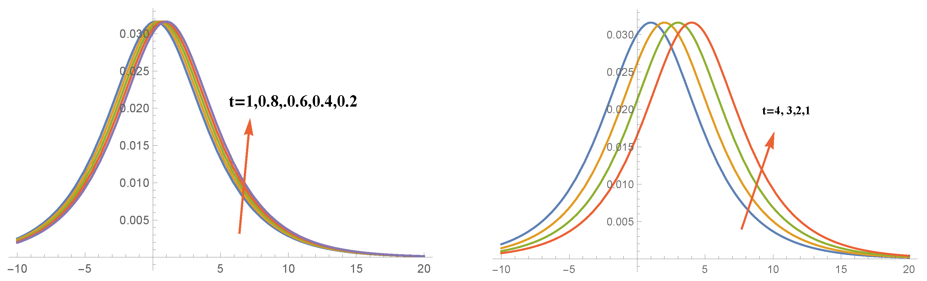
Example 2.

In this example, we will take the value of p that appeared in Equation (1) to be 3, while keeping the values $\mu ,ϵ$ as they are in the previous example.

We noticed from the graphics in the first example that the type of solution is of soliton types, but in this second example, a new feature called bifurcation will appear, where the wave starts to bifurcate into two waves after some time close to $t=0.4$, as shown in Figure 4.

Figure 4. The solution of Equation (1) using ADM when $p=3$ for different values of t.

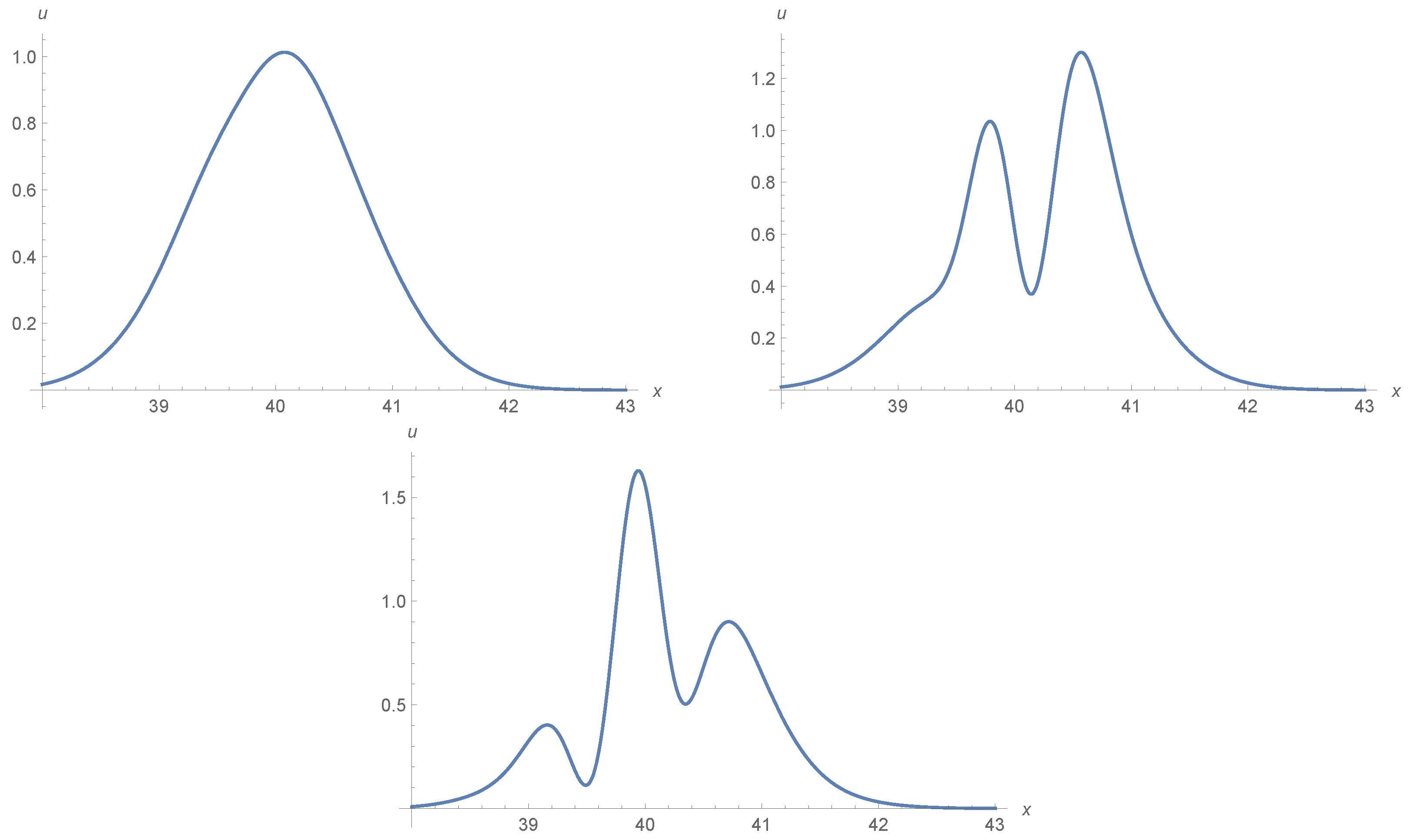
Example 3.

In this last example, we examined the evolution of an initial Maxwellian pulse into solitary waves, arising as the initial condition of the form

$$u(x,0)=exp[-{(x-40)}^2]$$

When solving Equation (1) for $p=2$, and $ϵ=6$. It is known that the behavior of the solution with the Maxwellian condition depends on the values of $\mu$. So, we study each of the three cases: $\mu =0.5$, where only a single soliton is generated as shown in Figure 5, and $\mu =0.05$. When $\mu$ is reduced more and more, such as in the case of $\mu =0.05$, two single solitons are generated as in Figure 5, and for the case $\mu =0.005$, the Maxwellian initial condition has decayed into three stable solitary waves as generated and shown in Figure 5.

Figure 5. The solution of Equation (1) using ADM when $p=2,ϵ=6$ when $t=2$ and $\mu =0.5$ (Single soliton), $\mu =0.05$ (two solitons), $\mu =0.005$ (three solitons).

7. Discussion and Conclusions

Two algorithms have been proposed to find a numerical solution to the MRLW equation, which often appears in physical applications. Whereas the first method, which is known as Sinc-collocation, is described in detail, with a simple proof of the stability of the obtained numerical solution, with an indication of an insufficient necessary condition. The other method, known as ADM, was presented in general first, and then the method was allocated to Equation (1). For the effectiveness of the two algorithms, we use one example with a known solution of soliton type, and the accuracy is investigated via the use of the $L_{\infty },L_2$ error norms. The numerical results we obtained in the last section prove the effectiveness and accuracy of the two methods to a large extent. However, we would like to point out that the Sinc method is numerical, and the solution was obtained and evaluated at some nodes. The scheme was found to be stable, and it converges exponentially in space direction. On the other hand, the other scheme used to solve the MRLW equation is ADM, which was found to be highly efficient, and it provides accurate approximate solutions without spatial discretization as in the Sinc method. We used a few terms from the series solution obtained by the ADM and obtained a suitable accuracy. However, we may easily increase the accuracy using ADM by adding more terms to the series. The biggest benefit of using this method is the speed of its convergence to the exact solution, as well as the ease of use. Finally, a Maxwellian initial condition was used, and the relationship between $\mu$ and the number of solitons was discussed.