A Combination of Fuzzy Techniques and Chow Test to Detect Structural Breaks in Time Series

Abstract

In a series of papers, we suggested a non-statistical method for the detection of structural breaks in a time series. It is based on the applications of special fuzzy modeling methods, namely Fuzzy transform (F-transform) and selected methods of Fuzzy Natural Logic (FNL). In this paper, we combine our method with the principles of the classical Chow test, which is a well-known statistical method for testing the presence of a structural break. The idea is to construct testing statistics similar to that of the Chow test which is formed from components of the first-degree F-transform. These components contain an estimation of the average values of the tangents (slopes) of the time series over an imprecisely specified time interval. In this paper, we illustrate our method and its statistical test on a real-time series and compare it with three classical statistical methods.

1. Introduction

Structural breaks in time series are sudden unexpected changes in their course triggered by a structural change in the system (for example, opening a new factory), by an attack from outside, or by some other outer cause. Unlike single outliers, structural breaks are characterized by a longer duration. There are various statistical methods for detection and testing whether a structural break occurs in the given time point, see [1,2,3,4,5], and also non-statistical methods such as genetic algorithms [6].

However, a structural break hardly occurs just at one point. It is a phenomenon lasting usually over several time points. Hence, we argue that techniques based on methods of fuzzy modeling are better suited for this purpose. In [7] and elsewhere, we presented an effective non-statistical method for finding structural breaks. It is based on the application of the so-called fuzzy transform (F-transform) in combination with methods of fuzzy natural logic (FNL). They enable us to detect intervals of specific monotonic behavior and to discover existing structural breaks in a time series. The main idea consists of the fact that the F-transform provides an estimation of the average value of the slope in an imprecisely specified time interval (cf. [8]). The former is then evaluated using a specific evaluative linguistic expression whose semantics is modeled inside FNL (for the details, see [9]). The method is very effective and we argue that it can find the real structural breaks. However, it is non-statistical and so it is a challenge to prove that the detected structural breaks can also be statistically verified. This is the topic of this paper. We modify the classical Chow test [1]. First, we form a modified null hypothesis stating that there is no structural break in the given area and then prove that it is rejected if a structural break is indeed present and detected using our fuzzy method.

The paper is structured as follows. Section 2 contains preliminaries in which we recall the principles of the Chow test, fuzzy transform, and the theory of evaluative linguistic expressions (as a part of FNL). In Section 3, we introduce the algorithm for finding structural breaks using our method, suggest modification of Chow test, and prove that if a structural break is detected then the null hypothesis stating that there is no structural break is rejected. Section 4 contains experimental verification of our results and also a comparison with three statistical techniques, namely the classical Chow, Bai-Perron, and Pettitt’s tests.

2. Preliminaries

2.1. Chow Test

This is one of the first statistical tests (see [1,4]) using which it is possible to decide whether we are facing a structural break or not. Its idea consists of splitting the data having n observations into two parts: $n_1$ observations before the break in time $t_0$ and $n_2$ observations after it. Then we construct two linear regressions models

$$\begin{array}{cc}\hfill y_1\left(t\right)& ={\alpha }_1+{\beta }_1{X}_1\left(t\right)+{\epsilon }_1,t=1,\dots ,n_1\hfill \\ \hfill y_2\left(t\right)& ={\alpha }_2+{\beta }_2{X}_2\left(t\right)+{\epsilon }_2,t=n_1+1,\dots ,n_1+n_2\hfill \end{array}$$

which are compared with the general regression model

$$y\left(t\right)=\alpha +\beta X\left(t\right)+\epsilon ,t=1,\dots ,n$$

($n=n_1+n_2$).

The ordinary least squares method is applied to the models above and then we form squares of residuals

• RSS₁ which is the residual of squares before the break:

  $${\mathrm{RSS}}_1=\sum _{t=1}^{n_1}{(y_1\left(t\right)-({\widehat{\alpha }}_1+{\widehat{\beta }}_1{X}_1\left(t\right)))}^2$$
• RSS₂ is the residual of squares after the break:

  $${\mathrm{RSS}}_2=\sum _{t=n_1+1}^{n_2}{(y_2\left(t\right)-({\widehat{\alpha }}_2+{\widehat{\beta }}_2{X}_1\left(t\right)))}^2$$
• RSS₃ is the residual of squares of the general regression model:

  $${\mathrm{RSS}}_3=\sum _{t=1}^n{(y\left(t\right)-(\widehat{\alpha }+\widehat{\beta }X\left(t\right)))}^2.$$

The test of hypothesis related to the test of structural break is conducted by testing the null hypothesis

$$H_0:{\alpha }_1={\alpha }_2,{\beta }_1={\beta }_2.$$

The structural change is caused due to different intercept terms as well as different regression coefficients. Under the assumption that the probability distribution of $y_1,y_2$ is normal, we can test the null hypothesis by the statistics

$$F_{test}=\frac{({\mathrm{RSS}}_3-({\mathrm{RSS}}_1+{\mathrm{RSS}}_2))/p}{({\mathrm{RSS}}_1+{\mathrm{RSS}}_2)/(n_1+n_2-2p)}$$

(1)

which has the F-distribution $F(p,n_1+n_2-2p)$. The null hypothesis $H_0$ is rejected if

$$F_{test}>F_{crit}$$

where $F_{crit}$ is a critical value of the F-distribution for a corresponding significance level $\alpha$ (as usual, we consider $\alpha \in \{0.1,0.05,0.01\}$).

2.2. Fuzzy Transform (F-Transform)

The fuzzy transform is a technique for the approximation of continuous functions. In our case, it can be effectively applied to analysis and forecasting of time series. Let a bounded real continuous function $f:[a,b]\to [c,d]$ be given, where $a,b,c,d\in \mathbb{R}$.

Definition 1. 

Let $c_0<\cdots <c_n$ be fixed nodes in the interval $[a,b]$ where $c_0=a$, $c_n=b$ with $n\ge 2$ and $a,b\in \mathbb{R}$. The set $\mathcal{A}=\{A_0,\dots ,A_n\}$ of fuzzy sets on $[a,b]$ is called a fuzzy partition of $[a,b]$ if the following conditions are fulfilled：

• $A_k:\left[a,b\right]\to \left[0,1\right]$, $A_k\left(c_k\right)=1$;
• $A_k\left(x\right)=0$ if $x\notin \left(c_{k-1},c_{k+1}\right)$ (for $c_{-1}=a$ and $c_{n+1}=b$ );
• $A_k$ is continuous;
• $A_k$ strictly increases on $[c_{k-1},c_k]$ for $k=1,\dots ,n$ and $A_k$ strictly decreases on $[c_k,c_{k+1}]$ for $k=0,\dots ,n-1$;
• $\sum _{k=0}^n{A}_k\left(x\right)=1$for all$x\in [a,b]$;
• If$c_k=a+hk$, where$h=(b-a)/n$, then fuzzy partition$\mathcal{A}$is called uniform and the following holds for the fuzzy sets forming it:$A_k(c_k-x)=A_k(c_k+x)$, $x\in [0,h]$, $A_k\left(x\right)=A_{k-1}(x-h)$, $A_{k+1}\left(x\right)=A_k(x-h)$where$k=1,\dots ,n-1$and$x\in [c_k,c_{k+1}]$.

The fuzzy sets $A_k\in \mathcal{A}$ are often called basic functions. Their shape can be arbitrary (but fulfilling Definition 1). Most often they are simple triangles. The F-transform has two phases: direct and inverse.

Definition 2. 

Let the set$\mathcal{A}=\{A_0,\dots ,A_n\}$be a uniform fuzzy partition with triangular basic functions, h be the distance between nodes and$f:[a,b]\to [c,d]$be a continuous function on$[a,b]$. The$(n+1)$-tuple$\mathbf{F}\left[f\right]=(F_0\left[f\right],\dots ,F_n\left[f\right])$is a direct fuzzy transform of f where the elements$F_0\left[f\right],\dots ,F_n\left[f\right]$are called components.

• The zero-degree fuzzy transform has components of the form

  $$F_k^0\left[f\right]=\frac{{\int }_a^{b}f\left(x\right)A_k\left(x\right)dx}{h},k=0,\dots ,n.$$

  (2)
• The first-degree fuzzy transform has components of the form

  $$F_k^1\left[f\right]\left(x\right)=({\beta }_k^0\left[f\right]+{\beta }_k^1\left[f\right]·(x-c_k))$$

  (3)

  where

  $$\begin{array}{cc}\hfill {\beta }_k^0\left[f\right]& =\frac{{\int }_{c_{k-1}}^{c_{k+1}}f\left(x\right)A_k\left(x\right)dx}{h},\hfill \end{array}$$

  (4)

  $$\begin{array}{cc}\hfill {\beta }_k^1\left[f\right]& =\frac{6{\int }_{c_{k-1}}^{c_{k+1}}f\left(x\right)(x-c_k)A_k\left(x\right)dx}{h^3}.\hfill \end{array}$$

  (5)

The coefficient ${\beta }_k^1\left[f\right]$ provides estimation of an average value of the tangent (slope) of f over the area characterized by the fuzzy set $A_k$.

Remark 1. 

Note that the coefficients ${\beta }_k^0\left[f\right]$ are identical with the components (2) of the zero-degree F-transform.

Definition 3. 

Let${\mathbf{F}}^m\left[f\right]=(F_0^m\left[f\right],\dots ,F_n^m\left[f\right])$be a direct F-transform of f due to Definition 2, where$m\in \{0,1\}$. (In fact, we can define F-transform of arbitrary degree. For our purposes, however, zero and first degrees are sufficient). The inverseF-transform of f is a function

$${\widehat{f}}_h^m\left(x\right)=\sum _{k=0}^n{F}_k^m\left[f\right]·A_k\left(x\right),x\in [a,b].$$

(6)

It can be proved that ${\widehat{f}}_h^m$ approximates the original function f with arbitrary precision (depending on h). We can set the parameters so that the approximating function ${\widehat{f}}_h^m$ has desired properties. The computational complexity of the F-transform is linear. More details can be found in [8,9,10].

2.3. Fuzzy Natural Logic

Our applications to time series require selected methods of Fuzzy Natural Logic (FNL). This is a class of mathematical models characterizing some parts of human common sense thinking that is based on the use of natural language. It includes, besides others, the theory of evaluative linguistic expressions and their semantics and fuzzy/linguistic IF-THEN rules. In a form suitable for time series processing is FNL described in [9]. In this section, we will recall some of the main points needed below.

Evaluative Linguistic Expressions (We will often omit the adjective “linguistic”.) are special expressions of natural language in the form

$$⟨\mathit{linguistichedge}⟩⟨\mathit{TE}-\mathit{adjective}⟩$$

(7)

where ⟨linguistic hedge⟩ is a special adverb standing before ⟨TE-adjective⟩, that makes the adjective more or less specific. We will consider linguistic hedges extremely (Ex), significantly (Si), very (Ve), rather (Ra), more or less (ML), roughly (Ro), very roughly (VR). The TE-adjectives are canonical adjectives zero (Ze), small (Sm), medium (Me), big (Bi). Note that they can be replaced by many other adjectives, for example shallow, medium deep, deep, etc.

Remark 2. 

Evaluative linguistic expressions (7) are called simple. We can introduce also complex ones that are formed using connective (and, or). Their syntax and semantics, however, are more complicated since they are not just boolean expressions. We need not consider them in this paper.

The model of the semantics of evaluative expressions requires the concept of context. In our case, this is the interval $w=[v_L,v_S]\cup [v_S,v_R]$ where $v_L,v_S,v_R\in R$. The numbers have the following meaning: $v_L$ is the left bound, $v_S$ is a typical middle value, and $v_R$ is the right bound.

Let $\mathcal{B}$ be an evaluative linguistic expression. The mathematical model of its meaning is a function $W\to \mathcal{F}\left(R\right)$ where W is a set of all contexts. Such a function is called intension of $\mathcal{B}$. If a context $w\in W$ is given then extension of $\mathcal{B}$ w.r.t. w is a fuzzy set from $\mathcal{F}\left(R\right)$. The details of this model are described in [9].

Let a value $x\in \mathbb{R}$ be given. We may now ask, what is a proper evaluative linguistic expression $\mathcal{B}$ using which we can characterize linguistically the value x? Of course, this depends on the context $w\in W$. For example, 100 USD may be a big money in a poor country but very small in a rich one. Therefore, we consider a special function of local perception

$$\mathcal{B}=LPerc(x,w)$$

(8)

which assigns an evaluative expression $\mathcal{B}$ to the value x w.r.t. the context $w\in W$. (Lperc is implemented in the special software LFL Forecaster described, e.g., in [9,11]).

A special class of evaluative expressions are those characterizing the trend of time series:

$$\mathrm{Trend}\mathrm{is}⟨\mathit{direction}⟩$$

(9)

where

• $⟨\mathit{direction}⟩$:= stagnating $\mid ⟨\mathit{specialhedge}⟩⟨\mathit{sign}⟩$,
• $⟨\mathit{sign}⟩$:= increasing ∣ decreasing,
• $⟨\mathit{specialhedge}⟩$: = ∅∣ negligibly ∣ slightly ∣ somewhat ∣ clearly ∣ roughly ∣ sharply ∣ quite largely ∣ fairly large∣ hugely∣ significantly.

We must also consider the context $w_{tg}$ for tangent that is here extended to have two parts: positive $w_{tg}^{+}$ for the increase in time series and negative $w_{tg}^{-}$ for its decrease.

3. Processing of Time Series Using Methods of Fuzzy Modeling

3.1. Processing of Time Series Using F-transform

A time series X is a mapping [12,13,14,15]

$$X:\mathbb{T}\times \Omega \to \mathbb{R},$$

where $\mathbb{T}$ is a set of numbers interpreted as time moments, $\Omega$ is a nonempty set of elementary random events and $(\Omega ,\mathcal{C},P)$ is a probability space, where $\mathcal{C}$ is a $\sigma$-algebra over $\Omega$ and P is a probability measure. In general, $\mathbb{T}\subset \mathbb{R}$ can be an arbitrary set. For our purposes, we will consider to be a finite set of natural numbers $T=\{0,\dots ,n\}\subset \mathbb{N}$.

We assume that the time series can be decomposed into 4 components, namely

$$X(\omega ,t)=\left(t\right)+C\left(t\right)+S\left(t\right)+R(\omega ,t),t\in T,\omega \in \Omega$$

(10)

where $Tr\left(t\right)$ and $C\left(t\right)$ are trend and cyclic components of the time series. These two components are usually combined into one component called trend-cycle $TC\left(t\right)=Tr\left(t\right)+C\left(t\right)$.

The $S\left(t\right)$ is the seasonal component and $R(\omega ,t)$ is a random noise. The trend, cycle and seasonal components are ordinary functions not having stochastic character. The noise $R(\omega ,t)$ is assumed to be a sequence of independent random variables with the mean $\mu =0$ and variance ${\sigma }^2<+\infty$.

It has been proved (see [9,16,17]) that using the F-transform, we can estimate trend Tr or trend-cycle TC with high fidelity which means that the seasonal component S is almost “wiped out” (i.e., its inverse F-transform is close to zero) and the noise R is significantly reduced [18].

3.2. Detection of Structural Breaks in a Time Series

Detection of a structural break in a time series means to determine a time interval in which the course of the time series abnormally changes in comparison with its previous/subsequent development. Our detection method presented in [7] is based on finding short intervals with a steep slope of trend (big tangent) preceded or followed by an interval with a small slope.

Let X be a time series, $\overline{\mathbb{T}}\subseteq T$ be a time interval. Let $\mathcal{A}$ be a basic function due to Definition 1 with the support $\overline{\mathbb{T}}$ over which ${\beta }^1\left[X\right|\overline{\mathbb{T}}]$ is the slope of the trend of X computed using (5). Let $w_{tg}^{-},w_{tg}^{+}$ be the corresponding negative and positive parts of the context, respectively. Then, the evaluative expression $\pm Ev\left[X|\overline{\mathbb{T}}\right]$ obtained using the function of local perception (8)

$$\pm Ev\left[X\right|\overline{\mathbb{T}}]=LPerc(\pm {\beta }^1\left[X\right|\overline{\mathbb{T}}],w_{tg}^{\pm }).$$

(11)

evaluates the trend of the time series X in the interval $\overline{\mathbb{T}}$. Using evaluation (11), we can decompose the time domain T into a set of intervals

$$\mathcal{T}=\{{\overline{T}}_i\mid i=1,\dots ,s\},\bigcup \mathcal{T}=\mathbb{T}$$

in which the slope is evaluated by specific evaluative expressions. The intervals need not necessarily be disjointed.

Definition 4. 

Let$\pm Ev\left[X\right|{\overline{\mathbb{T}}}_{i-1}],\pm Ev\left[X\right|{\overline{\mathbb{T}}}_i],\pm Ev\left[X\right|{\overline{\mathbb{T}}}_{i+1}]$be evaluative expressions computed using (11). An interval${\overline{\mathbb{T}}}_i\in \mathcal{T}$is an area of a structural break in the course of X if$\pm Ev\left[X\right|{\overline{\mathbb{T}}}_i]\in \{\pm Ve Bi,\pm Si Bi,\pm Ex Bi\}$and$\pm Ev\left[X\right|{\overline{\mathbb{T}}}_k]\in \{Ze,\pm Ve Sm$, $\pm Si Sm,\pm Ex Sm\}$where$k=i-1$or$k=i+1$.

This definition is the basis for the following algorithm for finding structural breaks in a time series X.

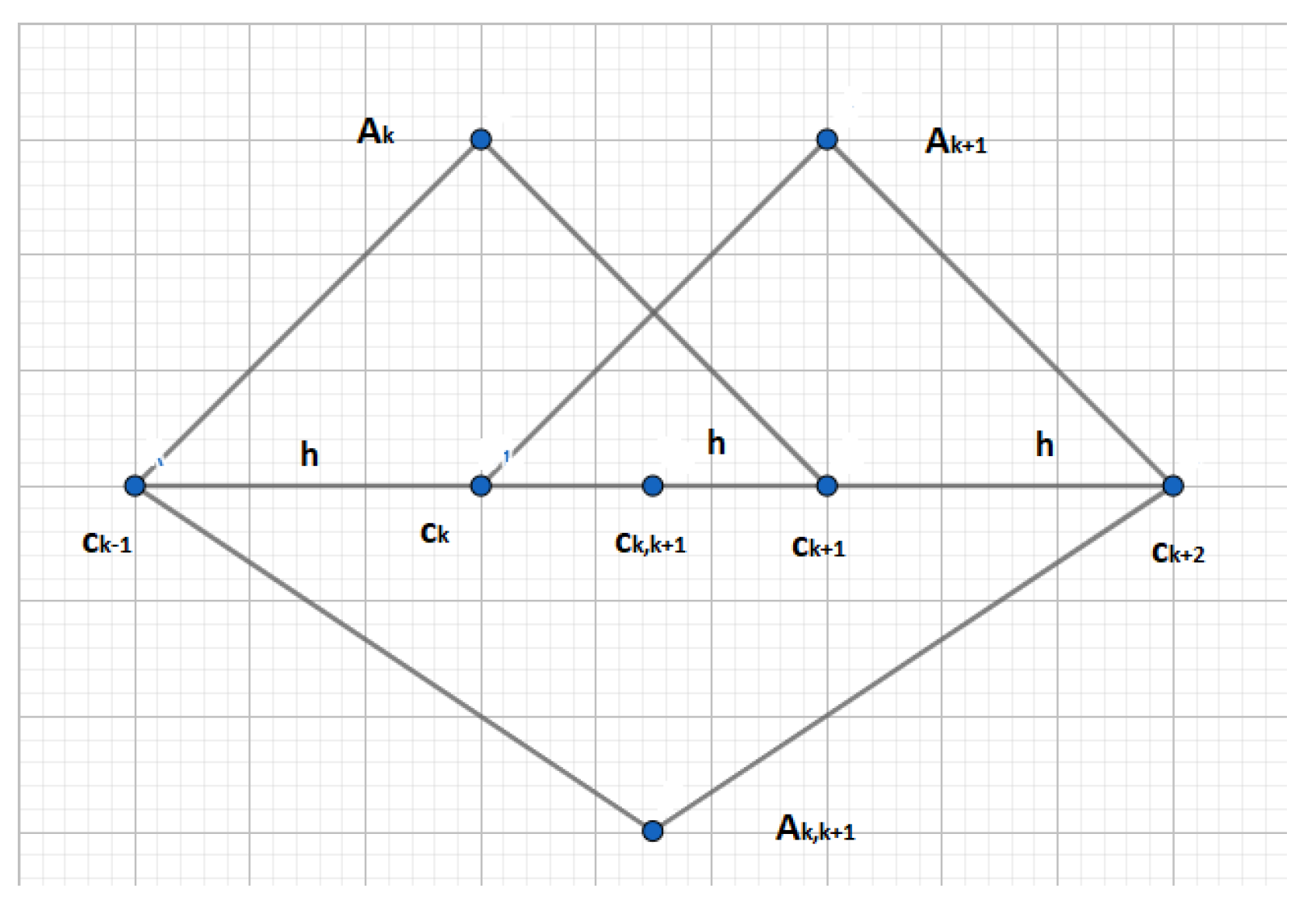
Algorithm for finding structural breaks

• Set the distance $h>0$ and determine a uniform fuzzy partition $\mathcal{A}$ over the time domain due to Definition 1.
• Set the context $w_{tg}^{-},w_{tg}^{+}$ for evaluation of the trend in the areas determined by the basic functions.
• Compute the direct first-degree fuzzy transform ${\mathbf{F}}^1\left[X\right]=(F_1^1\left[X\right],\dots ,F_{n-1}^1\left[X\right])$ over the fuzzy partition $\mathcal{A}$.
• Localize all pairs of components ($F_k^1\left[X\right]$,$F_{k+1}^1\left[X\right]$) (cf. (3)) with the following properties:

  –

  $LPerc({\beta }_k^1\left[X\right],w_{tg}^{\pm })\in \{Ze,$, $Ve Sm,Si Sm,Ex Sm\}$, i.e., the coefficient ${\beta }_k^1$ is close to zero.

  –

  $LPerc({\beta }_{k+1}^1\left[X\right],w_{tg}^{\pm })\in \{Ve Bi,Si Bi,Ex Bi\}$, i.e., the coefficient ${\beta }_{k+1}^1$ is unexpectedly big.

  Alternatively, k and $k+1$ can be interchanged, i.e., ${\beta }_{k+1}^1$ is close to zero and ${\beta }_k^1$ is unexpectedly big.
• The interval ${\mathbb{T}}_k$ (or ${\mathbb{T}}_{k+1}$) which is a support of the basic function $A_k\in \mathcal{A}$ (or $A_{k+1}\in \mathcal{A}$) is the area of a structural break due to Definition 4.

Without loss of generality, we will in the sequel assume that ${\beta }_k^1$ is close to zero and ${\beta }_{k+1}^1$ is unexpectedly big.

3.3. Combination of Fuzzy Techniques and Chow Test

Suppose that a time series X contains a structural break that occurs in the intersection of two adjacent areas represented by the triangular basic functions (fuzzy sets) $A_k$, $A_{k+1}\in \mathcal{A}$ in the sense of the algorithm presented in the previous section. Moreover, we also consider a third triangular basic function denoted by $A_{k,k+1}$ over the nodes $c_{k-1},c_{k+2}$ where the node

$$c_{k,k+1}=\frac{c_k+c_{k+1}}{2}$$

is added. Note that the fuzzy set $A_{k,k+1}$ is defined over nodes with the distance $\frac{3}{2}h$. The situation is depicted in Figure 1 (the fuzzy set $A_{k,k+1}$ is depicted upside-down for better visibility).

Figure 1. Fuzzy sets covering the structural break occurring in the interval $[c_k,c_{k+2}]$ (the support of the fuzzy set $A_{k+1}$).

Remark 3. 

The triangular fuzzy set $A_k$ w.r.t. the node $c_k$ is defined by the equation

$$A_k\left(t\right)=1-\frac{|t-c_k|}{h},t\in [c_{k-1},c_{k+1}]$$

and analogously also the fuzzy sets $A_{k+1}$ and $A_{k,k+1}$. Note also that

$$t-c_{k,k+1}=\frac{t-c_k}{2}+\frac{t-c_{k+1}}{2}.$$

Lemma 1. 

Let the triangular fuzzy sets depicted in Figure 1 be given. Then

$$A_{k,k+1}\left(t\right)\le A_k\left(t\right)+A_{k+1}\left(t\right)$$

for all $t\in T$.

Proof. 

It is enough to consider only the interval $[c_{k-1},c_{k+2}]$. By simple computation, we verify that $A_{k,k+1}\left(t\right)\le A_k\left(t\right)$ for $t\in [c_{k-1},c_k]$ and $A_{k,k+1}\left(t\right)\le A_{k+1}\left(t\right)$ for $t\in [c_{k+1},c_{k+2}]$. For $t\in [c_k,c_{k+1}]$ the inequality follows from the property $A_k\left(t\right)+A_{k+1}\left(t\right)=1$. □

Let us now consider the following F¹-transform components:

$$\begin{array}{cc}\hfill F_k^1\left[X\right]\left(t\right)& ={\beta }_k^0\left[X\right]+{\beta }_k^1\left[X\right]·(t-c_k),\hfill \end{array}$$

(12)

$$\begin{array}{cc}\hfill F_{k+1}^1\left[X\right]\left(t\right)& ={\beta }_{k+1}^0\left[X\right]+{\beta }_{k+1}^1\left[X\right]·(t-c_{k+1}),\hfill \end{array}$$

(13)

$$\begin{array}{cc}\hfill F_{k,k+1}^1\left[X\right]\left(t\right)& ={\beta }_{k,k+1}^0\left[X\right]+{\beta }_{k,k+1}^1\left[X\right]·(t-c_{k,k+1})\hfill \end{array}$$

(14)

where the coefficients ${\beta }^0,{\beta }^1$ are determined by the corresponding basic functions due to Figure 1.

Lemma 2. 

Let the triangular fuzzy sets depicted in Figure 1 be given. Then

$${\beta }_{k,k+1}^0\le {\beta }_k^0+{\beta }_{k+1}^0.$$

Proof. 

Using (4) and Lemma 1 we obtain

$$\begin{array}{c}{\beta }_{k,k+1}^0=\frac{1}{\frac{3}{2}h}{\int }_{c_{k-1}}^{c_{k+2}}X\left(t\right)A_{k,k+1}\left(t\right)dt\le \frac{1}{h}{\int }_{c_{k-1}}^{c_{k+2}}X\left(t\right)(A_k\left(t\right)+A_{k+1}\left(t\right))dt=\hfill \\ \hfill \frac{1}{h}{\int }_{c_{k-1}}^{c_{k+1}}X\left(t\right)A_k\left(t\right)dt+\frac{1}{h}{\int }_{c_k}^{c_{k+2}}X\left(t\right)A_{k+1}\left(t\right)dt={\beta }_k^0+{\beta }_{k+1}^0.\end{array}$$

□

Lemma 3. 

Let the triangular fuzzy sets depicted in Figure 1 be given. Then

$${\beta }_{k,k+1}^1\le {\beta }_k^1+{\beta }_{k+1}^1.$$

Proof. 

Using (5) and Lemma 1 we obtain

$$\begin{array}{c}{\beta }_{k,k+1}^1=\frac{6}{{\left(\frac{3}{2}h\right)}^3}{\int }_{c_{k-1}}^{c_{k+2}}X\left(t\right)(t-c_{k,k+1})A_{k,k+1}\left(t\right)dt\le \hfill \\ \frac{6}{h^3}{\int }_{c_{k-1}}^{c_{k+2}}X\left(t\right)(t-c_{k,k+1})(A_k\left(t\right)+A_{k+1}\left(t\right))dt=\\ \frac{1}{2}\left[\frac{6}{h^3}{\int }_{c_{k-1}}^{c_{k+1}}X\left(t\right)(t-c_k)A_k\left(t\right)dt+\frac{6}{h^3}{\int }_{c_{k-1}}^{c_{k+1}}X\left(t\right)(t-c_{k+1})A_k\left(t\right)dt\right]+\\ \frac{1}{2}\left[\frac{6}{h^3}{\int }_{c_k}^{c_{k+2}}X\left(t\right)(t-c_k)A_{k+1}\left(t\right)dt+\frac{6}{h^3}{\int }_{c_k}^{c_{k+2}}X\left(t\right)(t-c_{k+1})A_{k+1}\left(t\right)dt\right]=\\ \left[\frac{1}{2}{\beta }_k^1+\frac{1}{2}{\beta }_k^1-\frac{h}{2}\frac{6}{h^3}{\int }_{c_{k-1}}^{c_{k+1}}{A}_k\left(t\right)\right]+\left[\frac{1}{2}{\beta }_{k+1}^1+\frac{1}{2}{\beta }_{k+1}^1+\frac{h}{2}\frac{6}{h^3}{\int }_{c_k}^{c_{k+2}}{A}_k\left(t\right)\right]=\\ \hfill {\beta }_k^1-\frac{6}{h}+{\beta }_{k+1}^1+\frac{6}{h}={\beta }_k^1+{\beta }_{k+1}^1.\end{array}$$

□

Lemma 4. 

Let (12)–(14) be components of the F¹ transform according to the fuzzy partition depicted in Figure 1. Let ${\beta }_k^1=0$ and ${\beta }_{k+1}^1=K\ne 0$. Then ${\beta }_{k,k+1}^1\ne 0$.

Proof. 

It is sufficient to consider the interval $[c_{k+1},c_{k+2}]$, in which the fuzzy set $A_k\left(t\right)=0$ and, therefore, it cannot affect the size of ${\beta }_{k+1}^1$ and ${\beta }_{k,k+1}^1$ (cf. formula (5)).

Put $H=min\{X\left(t\right)\ne 0\mid t\in [c_{k+1},c_{k+2}]\}$. By the assumption, if there is a structural break over $[c_k,c_{k+2}]$ then $H\ne 0$ and it should be large since the corresponding $X\left(t\right)$ are not covered by the fuzzy set $A_k$ over which ${\beta }_k^1=0$ by the assumption. Then,

$$\begin{array}{cc}\hfill L& ={\int }_{c_{k+1}}^{c_{k+2}}H(t-c_{k+1})A_{k+1}\left(t\right)dt\le {\int }_{c_{k+1}}^{c_{k+2}}X\left(t\right)(t-c_{k+1})A_{k+1}\left(t\right)dt,\hfill \\ \hfill L^{\prime }& ={\int }_{c_{k+1}}^{c_{k+2}}H(t-c_{k,k+1})A_{k,k+1}\left(t\right)dt\le {\int }_{c_{k+1}}^{c_{k+2}}X\left(t\right)(t-c_{k,k+1})A_{k,k+1}\left(t\right)dt.\hfill \end{array}$$

After computation, we obtain $L=\frac{H{h}^2}{6}$ and $L^{\prime }=\frac{5H{h}^2}{18}$ which means that $0\ne L<L^{\prime }$. Consequently, ${\beta }_{k,k+1}^1\ne 0$. □

Let us now define the following sums of squares of differences between values of the time series and the F¹-transform components corresponding to the basic functions from Figure 1:

$$\begin{array}{cc}\hfill {\mathrm{RSS}}_k& =\sum _{t=c_{k-1}}^{c_{k+2}}{(X\left(t\right)-F_k^1\left[X\right]\left(t\right))}^2{A}_k\left(t\right),\hfill \end{array}$$

(15)

$$\begin{array}{cc}\hfill {\mathrm{RSS}}_{k+1}& =\sum _{t=c_{k-1}}^{c_{k+2}}{(X\left(t\right)-F_{k+1}^1\left[X\right]\left(t\right))}^2{A}_{k+1}\left(t\right),\hfill \end{array}$$

(16)

$$\begin{array}{cc}\hfill {\mathrm{RSS}}_{k,k+1}& =\sum _{t=c_{k-1}}^{c_{k+2}}{(X\left(t\right)-F_{k,k+1}^1\left[X\right]\left(t\right))}^2.\hfill \end{array}$$

(17)

Then, analogously to the classical Chow test (1) we construct the statistics

$$F_{test}=\frac{({\mathrm{RSS}}_{k,k+1}-({\mathrm{RSS}}_k+{\mathrm{RSS}}_{k+1}))/p}{({\mathrm{RSS}}_k+{\mathrm{RSS}}_{k+1})/(2n-2p)}$$

(18)

where n is the number of time points between $[c_{k-1},c_{k+2}]$ and p is the number of parameters (note that $p=2$ in our case). The statistics (18) has the F-distribution $F(p,2n-2p)$. The structural break is tested by the null hypothesis:

$$H_0:{\beta }_k^0={\beta }_{k+1}^0,{\beta }_k^1={\beta }_{k+1}^1.$$

(19)

The null hypothesis $H_0$ is rejected if $F_{test}>F_{crit}$ where $F_{crit}$ is a critical value.

The statistics (17) can be rewritten as

$$F_{test}=\frac{2(n-p)}{p}\left(\frac{{\mathrm{RSS}}_{k,k+1}}{{\mathrm{RSS}}_k+{\mathrm{RSS}}_{k+1}}-1\right).$$

(20)

We will refer to (18) or (20) as fuzzy Chow test.

Theorem 1. 

Let $X\left(t\right)$ be a time series over the time domain $\mathbb{T}$ and $\mathcal{A}$ be a uniform triangular fuzzy partition of with the distance h between nodes. Then

$$\left(\frac{{\mathrm{RSS}}_{k,k+1}}{{\mathrm{RSS}}_k+{\mathrm{RSS}}_{k+1}}\right)>1.$$

(21)

Proof. 

By ([8], Corollary 2), $X\left(t\right)=F_k^1\left(t\right)+O\left(h^2\right)$ for $t\in [c_{k-1},c_{k+1}]$. Then,

$${(X\left(t\right)-F_k^1\left(t\right))}^2\le M{h}^4$$

for some constant M and arbitrary h. Similar inequality holds also for $F_{k+1}^1$ and $t\in [c_k,c_{k+2}]$. Hence,

$${\mathrm{RSS}}_k+{\mathrm{RSS}}_{k+1}={\sum }_{t=c_{k-1}}^{c_{k+2}}{(X\left(t\right)-F_k^1\left(t\right))}^2{A}_k\left(t\right)+{\sum }_{t=c_{k-1}}^{c_{k+2}}{(X\left(t\right)-F_{k+1}^1\left(t\right))}^2{A}_{k+1}\left(t\right)<M^{\prime }{h}^4$$

(22)

for some constant $M^{\prime }$ and $t\in [c_{k-1},c_{k+2}]$. Considering a wider fuzzy partition with $h^{\prime }=\frac{3}{2}h$, in a similar way we obtain that

$${\mathrm{RSS}}_{k,k+1}=\sum _{t=c_{k-1}}^{c_{k+2}}{(X\left(t\right)-F_{k,k+1}^1\left[X\right]\left(t\right))}^2<M^{\prime }{\left(\frac{3}{2}h\right)}^4$$

(23)

(in both cases we can consider the same constant $M^{\prime }$). We argue that

$${\mathrm{RSS}}_k+{\mathrm{RSS}}_{k+1}<{\mathrm{RSS}}_{k,k+1}.$$

Indeed, let the opposite inequality hold. Then we choose h so that ${\mathrm{RSS}}_{k,k+1}<M^{\prime }{\left(\frac{3}{2}h\right)}^4<{\mathrm{RSS}}_k+{\mathrm{RSS}}_{k+1}$ and, by the assumption and (22), we obtain

$${\mathrm{RSS}}_{k,k+1}<M^{\prime }{\left(\frac{3}{2}h\right)}^4<{\mathrm{RSS}}_k+{\mathrm{RSS}}_{k+1}<M^{\prime }{h}^4$$

which is a contradiction. □

Theorem 2. 

Let $X\left(t\right)$ be a time series over the time domain $\mathbb{T}$ and $\mathcal{A}$ be a uniform triangular fuzzy partition of with the distance h between the nodes. Let $F_k^1,F_{k+1}^1$ be two components identifying structural break in the areas characterized by $A_k,A_{k+1}$ according to the algorithm presented in Section 3.2 (cf. Figure 1). Let

$$|X\left(t\right)-F_k^0\left(t\right)|\le \epsilon ,t\in [c_{k-1},c_{k+1}]and|X\left(t\right)-F_{k+1}^1\left(t\right)|\le \epsilon ,t\in [c_k,c_{k+2}].$$

(24)

If

$$\sum _{t\in [c_{k-1},c_{k+2}]}{(X\left(t\right)-F_{k,k+1}^1\left(t\right))}^2>m_h{\epsilon }^2$$

where $m_h$ is the number of time points between two nodes, then $F_{test}>>1$.

Proof. 

Let us consider formula (20) and denote the formulas after the sum symbol in (15)–(17) by ${\mathrm{RSS}}_k\left(t\right)$, ${\mathrm{RSS}}_{k+1}\left(t\right)$, ${\mathrm{RSS}}_{k,k+1}\left(t\right)$, respectively.

(a) Let $t\in [c_{k-1},c_k]$. Then

$${\mathrm{RSS}}_{k+1}\left(t\right)=0\mathrm{and}\sum _{t\in [c_{k-1},c_k]}{\mathrm{RSS}}_k\left(t\right)\le m_h{\epsilon }^2,$$

i.e., ${\sum }_{t\in [c_{k-1},c_k]}{\mathrm{RSS}}_k\left(t\right)+{\sum }_{t\in [c_{k-1},c_k]}{\mathrm{RSS}}_{k+1}\left(t\right)\le m_h{\epsilon }^2$. Similarly we obtain

$$\sum _{t\in [c_{k+1},c_{k+2}]}{\mathrm{RSS}}_k\left(t\right)+\sum _{t\in [c_{k+1},c_{k+2}]}{\mathrm{RSS}}_{k+1}\left(t\right)\le m_h{\epsilon }^2.$$

(b) Let $t\in [c_k,c_{k+1}]$. Then

$$\begin{array}{c}\sum _{t=c_k}^{c_{k+1}}{(X\left(t\right)-F_k^1\left[X\right]\left(t\right))}^2{A}_k\left(t\right)+\sum _{t=c_k}^{c_{k+1}}{(X\left(t\right)-F_{k+1}^1\left[X\right]\left(t\right))}^2{A}_k\left(t\right)\le \hfill \\ \hfill \sum _{t=c_k}^{c_{k+1}}({\epsilon }^2{A}_k\left(t\right)+{\epsilon }^2{A}_{k+1}\left(t\right))=m_h{\epsilon }^2.\end{array}$$

Consequently,

$$\sum _{t=c_{k-1}}^{c_{k+2}}{\mathrm{RSS}}_k\left(t\right)+\sum _{t=c_{k-1}}^{c_{k+2}}{\mathrm{RSS}}_{k+1}\left(t\right)\le m_h{\epsilon }^2.$$

(25)

Using the assumption, we thus obtain

$$1<\frac{{\mathrm{RSS}}_{k,k+1}}{m_h{\epsilon }^2}\le \frac{{\mathrm{RSS}}_{k,k+1}}{{\mathrm{RSS}}_k+{\mathrm{RSS}}_{k+1}}.$$

Realizing that for $p=2$, the multiplicative constant in (20) can be fairly high, the value of $F_{test}$ is also high. □

So far, we did not see whether our method for detection of the structural breaks has an impact on the statistics (20). In the following theorem we will show that when detecting a structural break using the algorithm from Section 3.2, the nominator of (20) significantly increases. For this purpose, we consider two time series $X,X^{\prime }$ which differ only in the interval $t\in [c_{k,k+1},c_{k+2}]$ where the structural break occurs, i.e., $X^{\prime }\left(t\right)=X\left(t\right)$ for $t\in [c_{k-1},c_{k,k+1}]$. We will denote the formulas (15)–(17) for the time series $X^{\prime }$ by ${\mathrm{RSS}}_k^{\prime },{\mathrm{RSS}}_{k+1}^{\prime },{\mathrm{RSS}}_{k,k+1}^{\prime }$, respectively.

In the proof of the following theorem, we meet the formula

$$W=\sum _{[c_{k-1},c_{k+2}]}{(t-c_{k,k+1})}^2=\frac{1}{2}{m}_h(\frac{3}{2}{m}_h+1)(3m_h+1).$$

Theorem 3. 

Let $m_h$ be the number of time points between two nodes. Furthermore, we will assume:

(a)

${\beta }_k^1\left[X\right]={\beta }_{k,k+1}^1\left[X\right]={\beta }_{k+1}^1\left[X\right]=0$,

(b)

the inequalities (24) hold for some $\epsilon >0$,

(c)

$|{\beta }_{k+1}^1\left[X^{\prime }\right]|>0$,

(d)

there are minimal ${\epsilon }^{\prime },{\epsilon }^{″}>0$ such that the following holds:

$$\begin{array}{cc}\hfill & max\left\{\right|X\left(t\right)-X\left(c_{k,k+1}\right)|\mid t\in [c_{k-1},c_{k+2}]\}\le \frac{{\epsilon }^{\prime }}{2},\hfill \\ \hfill & max\left\{\right|X^{\prime }\left(t\right)-X^{\prime }\left(c_{k,k+1}\right)|\mid t\in [c_{k-1},c_{k+2}]\}\le \frac{{\epsilon }^{″}}{2}.\hfill \end{array}$$

If the slope ${\beta }_{k,k+1}^1\left[X^{\prime }\right]$ fulfills the inequality

$$|{\beta }_{k,k+1}^1\left[X^{\prime }\right]|\ge \frac{{\sum }_{[c_{k-1},c_{k+2}]}|t-c_{k,k+1}|·|X\left(t\right)-{\beta }_{k,k+1}^0\left[X\right]|}{W}$$

(26)

then

$${\mathrm{RSS}}_{k,k+1}\le {\mathrm{RSS}}_{k,k+1}^{\prime }.$$

(27)

Proof. 

Note that $X^{\prime }\left(c_{k,k+1}\right)=X\left(c_{k,k+1}\right)$ and so, it follows from the assumptions (c), (d) that ${\epsilon }^{\prime }<{\epsilon }^{″}$ because (c) says that there is a structural break in $[c_k,c_{k+2}]$. Therefore, there must be $t_0\in [c_k,c_{k+2}]$ such that $|X^{\prime }\left(t_0\right)-X\left(c_{k,k+1}\right)|>{\epsilon }^{\prime }$.

In the same way as is in the proof of ([10], Theorem 5), we can show that

$$|X\left(t\right)-{\beta }_{k,k+1}^0\left[X\right]|\le {\epsilon }^{\prime },\mathrm{and}|X^{\prime }\left(t\right)-{\beta }_{k,k+1}^0\left[X^{\prime }\right]|\le {\epsilon }^{″}$$

for $t\in [c_{k-1},c_{k+2}]$. Then we have

$$\begin{array}{c}\sum _{t\in [c_{k-1},c_{k+2}]}{(X\left(t\right)-{\beta }_{k,k+1}^0\left[X\right])}^2\le 3m_h{{\epsilon }^{\prime }}^2<\sum _{t\in [c_{k-1},c_{k+2}]}{(X\left(t\right)-{\beta }_{k,k+1}^0\left[X^{\prime }\right])}^2-\hfill \\ \hfill 2|{\beta }_{k,k+1}^1\left[X^{\prime }\right]|\sum _{t\in [c_{k-1},c_{k+2}]}|t-c_{k,k+1}|·|X\left(t\right)-{\beta }_{k,k+1}^0\left[X^{\prime }\right]|+{\left({\beta }_{k,k+1}^1\left[X^{\prime }\right]\right)}^2\sum _{t\in [c_{k-1},c_{k+2}]}{(t-c_{k,k+1})}^2.\end{array}$$

The third inequality is assured if

$$\begin{array}{c}2|{\beta }_{k,k+1}^1\left[X^{\prime }\right]|·\sum _{t\in [c_{k-1},c_{k+2}]}|t-c_{k,k+1}|·|X\left(t\right)-{\beta }_{k,k+1}^0\left[X^{\prime }\right]|\le \hfill \\ \hfill {\left({\beta }_{k,k+1}^1\left[X^{\prime }\right]\right)}^2\sum _{t\in [c_{k-1},c_{k+2}]}{(t-c_{k,k+1})}^2,\end{array}$$

which implies that

$$|{\beta }_{k,k+1}^1\left[X^{\prime }\right]|\ge \frac{{\sum }_{[c_{k-1},c_{k+2}]}|t-c_{k,k+1}|·|X\left(t\right)-{\beta }_{k,k+1}^0\left[X\right]|}{W}.$$

This assures inequality (27). □

In this theorem, assumption (b) says that $F_k^0\left(t\right)$ and $F_{k+1}^1\left(t\right)$ well approximate X and $X^{\prime }$, respectively. Note that due to assumption (a), we may consider only $F_k^0$ instead of $F_k^1\left(t\right)$. Note that Lemma 4 justifies assumption (c); assumption (d) is justified by the results of [8,10].

Corollary 1. 

There is a context $w_{tg}=⟨0,v_S,v_R⟩$ such that $LPerc({\beta }_k^1\left[X^{\prime }\right],w_{tg})\in \left\{zero\right\}$ and LPerc$({\beta }_{k+1}^1\left[X^{\prime }\right],w_{tg})\in \left\{big\right\}$ and the null hypothesis using the fuzzy Chow-test for the time series $X^{\prime }$ is rejected.

Proof. 

We take the context $w_{tg}$ such that $v_S$ is equal to the right-hand side of (26) and $v_R$ big enough to assure that ${\beta }_{k+1}^1\left[X^{\prime }\right]$ is in (11) evaluated as big. Following the proof of Theorem 2, we can assure that (21) holds true and, consequently, that $F_{test}$ in (20) is sufficiently large. □

4. Experiments

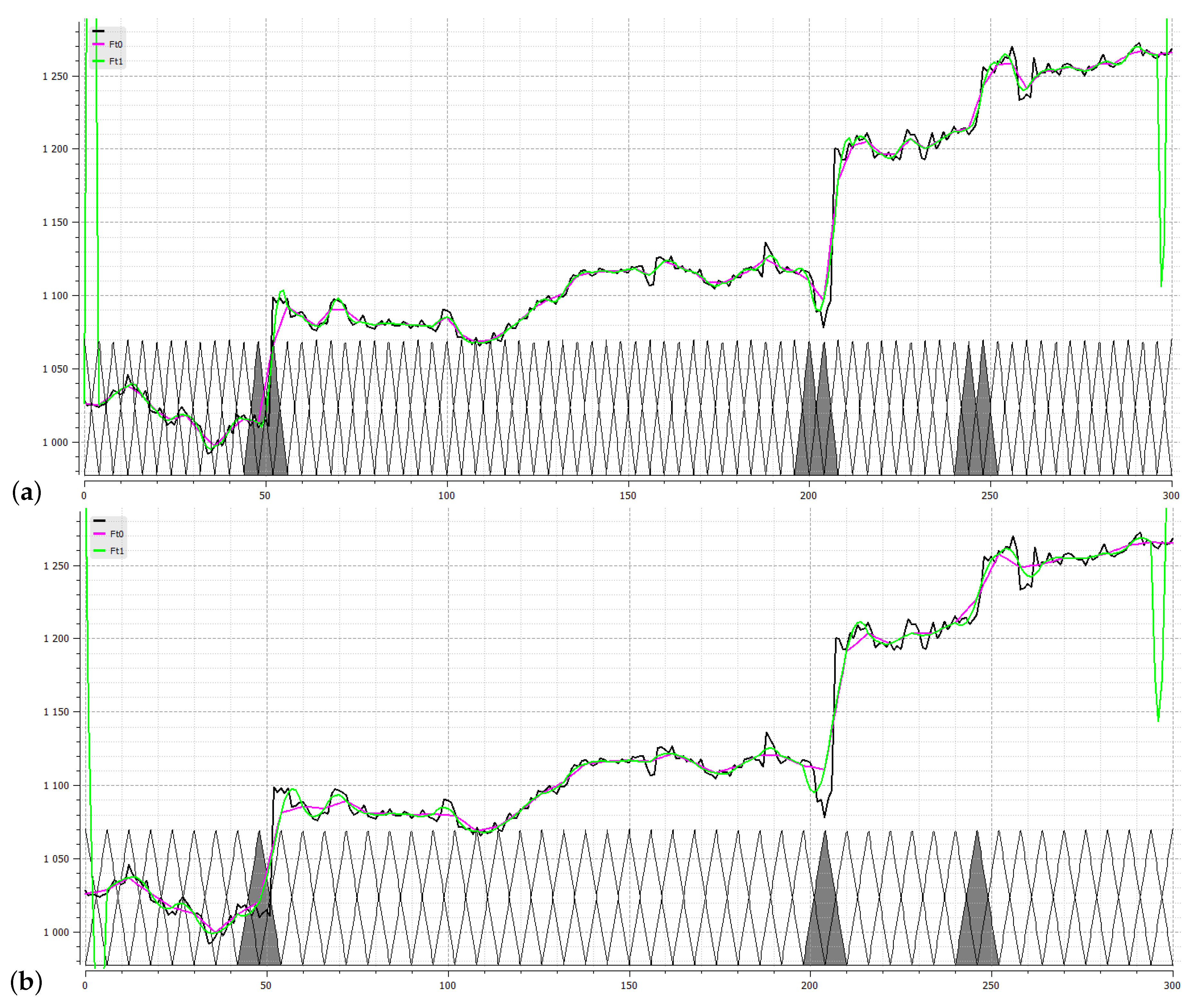
4.1. Detection of Structural Breaks

We will demonstrate our results on real data taken from a Micro subset of time series from M4-Competition published on the Internet. For computations of the F-transform components, we used the experimental software FT-studio. (It was developed in the Institute for Research of Applications of Fuzzy Modeling of the University of Ostrava, Czech Republic. Its author is Radek Valášek. Let us remark that in the R-repository is available R-package lfl providing algorithms used in this paper, see [19].).

In Figure 2, a real time series is depicted together with two fuzzy partitions with equidistant triangular basic functions. The structural breaks are detected using our method. Namely, the time series contains structural breaks occurring in areas characterized by couples of fuzzy sets $(A_{48}$, $A_{52}$), ($A_{204}$, $A_{208}$), ($A_{244}$, $A_{248}$).

Figure 2. The time series is depicted together with fuzzy partitions with the basic functions of the width: (a) $2h=8$ and (b) $2h=12$. In both images are marked basic functions over which the structural breaks are detected.

We apply Fuzzy Chow test to the found structural breaks using fuzzy technique. The first one is obtained from two F¹-transform components

$$\begin{array}{c}\hfill F_{48}^1\left[X\right]={\beta }_{48}^0\left[X\right]+{\beta }_{48}^1\left[X\right]·(t-c_{48})=1013.19-0.38·(t-48),\\ \hfill F_{52}^1\left[X\right]={\beta }_{52}^0\left[X\right]+{\beta }_{52}^1\left[X\right]·(t-c_{52})=1065.41+20.83·(t-52).\end{array}$$

To verify the found structural break also statistically, we will test the null hypothesis

$$H_0:{\beta }_{48}^0\left[X\left(t\right)\right]={\beta }_{52}^0\left[X\left(t\right)\right]and{\beta }_{48}^1\left[X\left(t\right)\right]={\beta }_{52}^1\left[X\left(t\right)\right]$$

The squares of residuals ${\mathrm{RSS}}_{48}$, ${\mathrm{RSS}}_{52}$, ${\mathrm{RSS}}_{48,52}$ are computed as follows:

$$\begin{array}{c}\hfill {\mathrm{RSS}}_{48}=\sum _{t=44}^{56}{(X_t-F_{48}^1\left[X\right]\left(t\right))}^2·A_{48}\left(t\right)=38.9604,\\ \hfill {\mathrm{RSS}}_{52}=\sum _{t=44}^{56}{(X_t-F_{52}^1\left[X\right]\left(t\right))}^2·A_{52}\left(t\right)=2441.03,\\ \hfill {\mathrm{RSS}}_{48,52}=\sum _{t=44}^{56}{(X_t-F_{48,52}^1\left[X\right]\left(t\right))}^2=9406.196.\end{array}$$

The Fuzzy Chow test is based on the statistics

$$F_{test}=\frac{({\mathrm{RSS}}_{48,52}-{\mathrm{RSS}}_{48}-{\mathrm{RSS}}_{52})/p}{({\mathrm{RSS}}_{48}+{\mathrm{RSS}}_{52})/(2n-2p)}=30.72$$

where $n=13$ and $p=2$.

We obtain $F_{test}=30.72>F_{crit}=F(p,2n-2p)=4.3828$ for $\alpha =0.025$ and so, we reject the null hypothesis. This means that we have sufficient evidence to say that a structural break detected using our method indeed occurs in the interval $t\in [44,56]$.

We apply the same algorithm with two subsequent by fuzzy sets ($A_{204}$, $A_{208}$) and ($A_{244}$, $A_{248}$), the structural breaks confirmed by testing the null hypothesis:

$$\begin{array}{cc}\hfill H_0:& {\beta }_{204}^0\left[X\left(t\right)\right]={\beta }_{208}^0\left[X\left(t\right)\right]and{\beta }_{204}^1\left[X\left(t\right)\right]={\beta }_{208}^1\left[X\left(t\right)\right],\hfill \\ \hfill H_0:& {\beta }_{244}^0\left[X\left(t\right)\right]={\beta }_{248}^0\left[X\left(t\right)\right]and{\beta }_{244}^1\left[X\left(t\right)\right]={\beta }_{248}^1\left[X\left(t\right)\right].\hfill \end{array}$$

The results are summarized in Table 1.

Table 1. Fuzzy Chow Test results.

t	Fuzzy Sets $[{\mathit{A}}_{\mathit{k}},{\mathit{A}}_{\mathit{k}+1}]$	${\mathit{F}}_{\mathit{test}}$	${\mathit{F}}_{\mathit{crit}}$ ($\mathit{\alpha }=0.025$)	Decision
[44,56]	[$A_{48},A_{52}$]	30.72	4.3828	Reject $H_0$
[200,212]	[$A_{204},A_{208}$]	26.52	4.3828	Reject $H_0$
[240,252]	[$A_{244},A_{248}$]	39.77	4.3828	Reject $H_0$

All of the results show that we have sufficient evidence to demonstrate that structural breaks occur in the data in the time intervals stated above.

4.2. When Fuzzy Chow Test Does Not Reject the Null Hypothesis?

Our method for detection of structural breaks is non-statistical. Therefore, we should also check whether the fuzzy Chow test does not falsely accept the null hypothesis about the existence of a structural break in place where our method detects none.

For example, lets us check time intervals $[80,92]$, $[112,124]$, $[152,164]$, $[228,240]$ characterized by fuzzy sets ($A_{84}$, $A_{88}$), ($A_{116}$, $A_{120}$), ($A_{156}$, $A_{160}$), ($A_{232}$, $A_{236}$) where no structural break is detected. We apply Fuzzy Chow test and so, we compute two F-transform components:

$$\begin{array}{c}\hfill F_{84}^1\left[X\right]={\beta }_{84}^0\left[X\right]+{\beta }_{84}^1\left[X\right]·(t-c_{84}),\\ \hfill F_{88}^1\left[X\right]={\beta }_{88}^0\left[X\right]+{\beta }_{88}^1\left[X\right]·(x-c_{88})\end{array}$$

and form the null hypothesis:

$$H_0:{\beta }_{84}^0\left[X\right]={\beta }_{88}^0\left[X\right]and{\beta }_{84}^1\left[X\right]={\beta }_{88}^1\left[X\right]$$

The statistics of the Fuzzy Chow test is

$$F_{test}=\frac{({\mathrm{RSS}}_{84,88}-{\mathrm{RSS}}_{84}-{\mathrm{RSS}}_{88})/p}{({\mathrm{RSS}}_{84}+{\mathrm{RSS}}_{88})/(2n-2p)}=3.13$$

where $n=13$ and $p=2$.

We may verify that $F_{test}=3.13<F_{crit}=F(p,2n-2p)=4.3828$ for $\alpha =0.025$. Hence, we cannot reject the null hypothesis. This means that we have no sufficient evidence to say that a structural break occurs in the interval $[80,92]$.

Let us apply same algorithm with fuzzy sets ($A_{116}$, $A_{120}$), ($A_{156}$, $A_{160}$) and ($A_{236}$, $A_{240}$) and form the following null hypotheses:

$$\begin{array}{cc}\hfill H_0:& {\beta }_{116}^0\left[X\right]={\beta }_{120}^0\left[X\right]and{\beta }_{116}^1\left[X\right]={\beta }_{120}^1\left[X\right],\hfill \\ \hfill H_0:& {\beta }_{156}^0\left[X\right]={\beta }_{160}^0\left[X\right]and{\beta }_{156}^1\left[X\right]={\beta }_{160}^1\left[X\right],\hfill \\ \hfill H_0:& {\beta }_{236}^0\left[X\right]={\beta }_{240}^0\left[X\right]and{\beta }_{236}^1\left[X\right]={\beta }_{240}^1\left[X\right].\hfill \end{array}$$

The results are summarized in Table 2.

Table 2. Fuzzy Chow Test results and Decisions.

Time Interval	Fuzzy Sets $({\mathit{A}}_{\mathit{k}},{\mathit{A}}_{\mathit{k}+1})$	${\mathit{F}}_{\mathbf{test}}$	${\mathit{F}}_{\mathbf{crit}}$ ($\mathit{\alpha }=0.025$)	Decision
[112,124]	$(A_{116},A_{120})$	2.81	4.3828	$H_0$ is not rejected
[152,164]	$(A_{156},A_{160})$	1.46	4.3828	$H_0$ is not rejected
[232,244]	$(A_{236},A_{240})$	1.86	4.3828	$H_0$ is not rejected

We conclude that the fuzzy Chow test indeed statistically verifies structural breaks only on places in which our method described in Section 3.2 detects them.

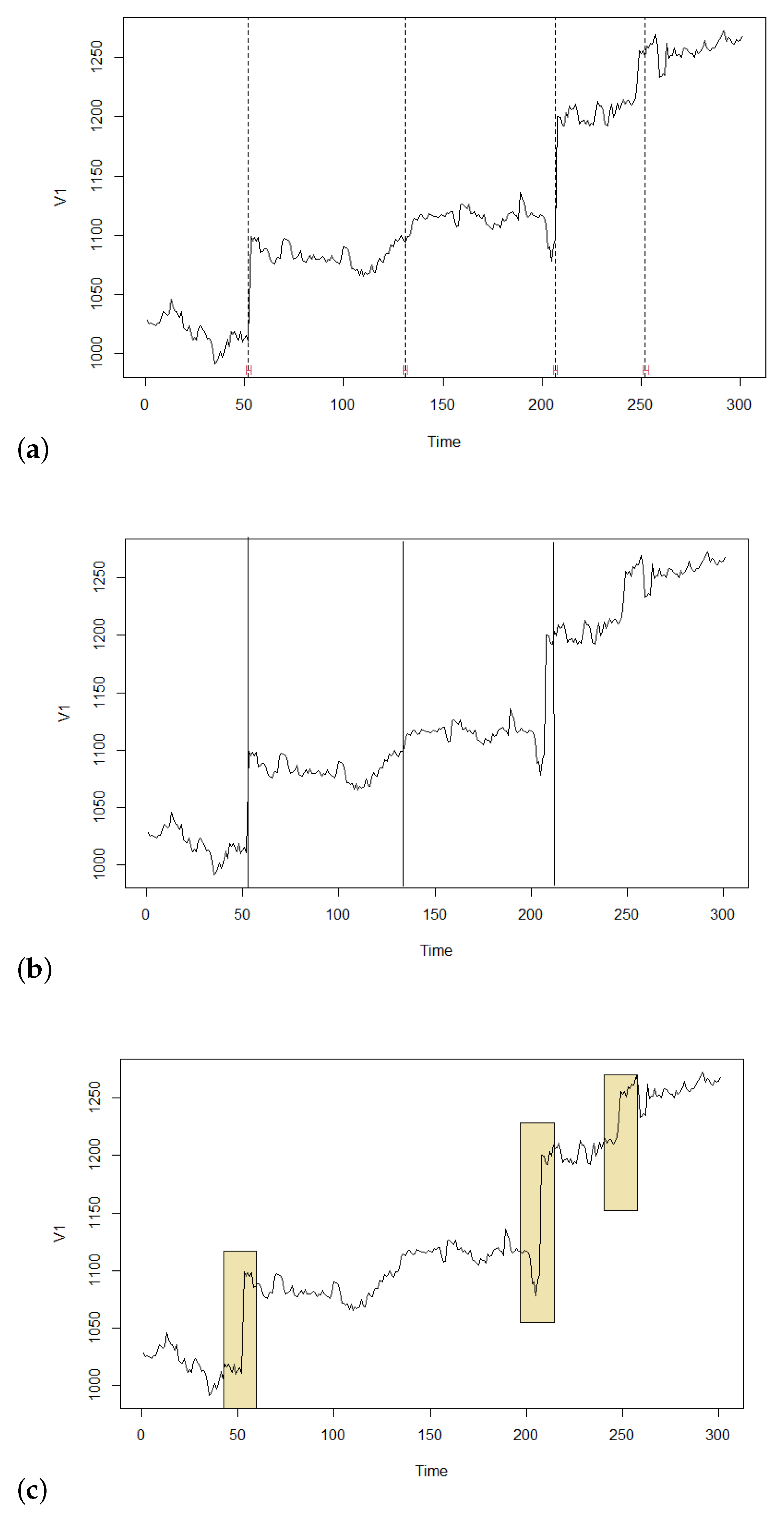
4.3. Comparison with Classical Statistical Tests

In this section, we will compare our method with three classical statistical methods for the detection of structural breaks. Namely, we will consider the classical Chow test described in Section 2.1, Pettitt’s, and Bai-Perron tests.

4.3.1. Pettitt’S Test (1979)

The Pettitt’s test [20,21] is a way to find out when there was a big change in the mean of a set of numbers over time when the exact time of the change is unknown. The data collect n observations, and if it contains a change point at time t, then the change point will split the data into two parts, each of which has a distinct distribution $F_1\left(x\right)$ and $F_2\left(x\right)$. The test statistic K is defined by $K=max\left|U_t\right|$ where

$$U_t=\sum _{i=1}^t\sum _{j=t+1}^n(x_i-x_j)\mathrm{and}\mathrm{sign}(x_i-x_j)=\left\{\begin{array}{cc}1\hfill & \mathrm{if}(x_i-x_j)>0,\hfill \\ 0\hfill & \mathrm{if}(x_i-x_j)=0,\hfill \\ -1\hfill & \mathrm{if}(x_i-x_j)<0.\hfill \end{array}\right.$$

The confidence level for n samples is $p=exp\left(\frac{-K}{n^2+n^3}\right)$. The null hypothesis is rejected if the value of p does not exceed the given confidence level.

4.3.2. Bai-Perron Test (1998)

Another well known test for identification of several structural breaks in a time series is Bai-Perron one [22,23,24].

With the null hypothesis: There is no structural break in the time series, the Bai-Perron proccess suggests a multiple linear regression with k changes. The change points are $(T_1,\dots ,T_k)$ and are explicitly handled as unknown:

$$\begin{array}{cc}\hfill y_t& =x_t\beta +z_t{\sigma }_1+{\epsilon }_t,t=1,\dots ,T_1,\hfill \\ \hfill y_t& =x_t\beta +z_t{\sigma }_2+{\epsilon }_t,t=T_1+1,\dots ,T_2,\hfill \\ \hfill & ....................\hfill \\ \hfill y_t& =x_t\beta +z_t{\sigma }_{k+1}+{\epsilon }_t,t=T_{k+1},\dots ,T\hfill \end{array}$$

where $y_t$ is the dependent variable, $\beta$ and $\sigma$ are coefficients corresponding to covariates $x_t$ and $z_t$, and $u_t$ is the residue term. The purpose is to estimate the unknown regression coefficients and the break dates $(\beta ,{\sigma }_1,\dots ,{\sigma }_{k+1},T_1,\dots ,T_k)$ when T observations on $(y_t,x_t,z_t)$ are given.

4.3.3. Comparison of Statistical Methods with Fuzzy Chow Test

The results of the comparison can be seen in Figure 3. The computations have been performed using R. The classical Chow test detected change points in $t=51,130,206,251$ and Bai-Perron test in $t=52,131,207,252$. Thus, the differences in the graph in Figure 3 are invisible. The Pettitt test found only three points in $t=51,130,206$.

Figure 3. Results of statistical tests as well as of our method to finding structural breaks in the real time series: (a) Chow and Bai-Perron tests (in the graph, there is no visible difference between them), (b) Pettitt’s test, and (c) our method verified by the fuzzy Chow test.

Our method detected three structural breaks in the intervals $[44,56]$, $[200,212]$, $[240,252]$ which, as shown in Section 4.1, are also statistically significant by the fuzzy Chow test. Note that these intervals cover the points found by Chow and Bai-Perron tests with the exception of $t=130$ ($t=131$) where, however, there is no structural break. We argue that, as is apparent from Figure 3, our method correctly detected real structural breaks occurring in the time series. The following conclusions imply from the comparison with our method:

• Statistical methods detect the breaks as if occurring in one time point. However, it is clear from the practice that this rarely happens; the break usually shows in a wider area. Hence, the result of a statistical test should be taken as a point around which the break occurs. But this is equal to what our fuzzy method provides explicitly, and thus we argue that more realistically.
• Statistical methods are less robust and thus, more sensitive to the data. Hence, they are prone to the detection of non-existing breaks. In our example, this happened to all three statistical methods in point $t=130$ ($t=131$) where apparently there is no structural break. Let us emphasize that our fuzzy method ignored this point/area due to its robustness.
• Statistical methods require optimization and therefore, they are computationally expensive. Our method is very simple and computationally effective since the fuzzy transform has linear complexity.

It is important to emphasize that our goal is not to beat statistical methods. Vice-versa, we want to employ maximally the synergy of both approaches.

5. Conclusions

In this paper, we focus on methods for the detection of structural breaks in time series. In [7], we suggested a method based on the fuzzy transform (F-transform) and selected methods of Fuzzy Natural Logic. In this paper, we suggested a combination of our method with a statistical text that stems from the well-known Chow test [1]. Statistical significance is demonstrated on the data. We have shown that our technique is effective in spotting abnormalities and gives statistically significant results. Further research will be focused on the combination of our fuzzy method with other kinds of statistical testing.

References

1. Chow, G.C. Tests of Equality Between Sets of Coefficients in Two Linear Regressions. Econometrica 1960, 28, 591–605. [Google Scholar] [CrossRef] [Green Version]
2. De Wachter, S.; Tzavalis, D. Detection of structural breaks in linear dynamic panel data models. Comput. Stat. Data Anal. 2012, 56, 3020–3034. [Google Scholar] [CrossRef] [Green Version]
3. Fischer, P.; Hilbert, A. Fast detection of structural breaks. In Proceedings of the 21th International Conference on Computational Statistics, Geneva, Switzerland, 19–22 August 2014; pp. 9–16. [Google Scholar]
4. Nielsen, B.; Whitby, A. A Joint Chow Test for Structural Instability. Econometrics 2015, 3, 156–186. [Google Scholar] [CrossRef] [Green Version]
5. Preuss, P.; Puchstein, R.; Detter, H. Detection of multiple structural breaks in multivariate time series. J. Am. Stat. Assoc. 2015, 110, 654–668. [Google Scholar] [CrossRef] [Green Version]
6. Doerr, B.; Fischer, P.; Hilbert, A.; Witt, C. Detecting structural breaks in time series via genetic algorithms. Soft Comput. 2017, 21, 4707–4720. [Google Scholar] [CrossRef]
7. Truong, P.; Novák, V. An Improved Forecasting and Detection of Structural Breaks in Time Series using Fuzzy Techniques. In Theory and Applications of Time Series Analysis and Forecasting; Valenzuela, O., Rojas, F., Herrera, L., Pomares, H., Rojas, I., Eds.; Springer: Berlin/Heidelberg, Germany, 2022. [Google Scholar]
8. Perfilieva, I.; Daňková, M.; Bede, B. Towards a Higher Degree F-transform. Fuzzy Sets Syst. 2011, 180, 3–19. [Google Scholar] [CrossRef]
9. Novák, V.; Perfilieva, I.; Dvořák, A. Insight into Fuzzy Modeling; Wiley & Sons: Hoboken, NJ, USA, 2016. [Google Scholar]
10. Perfilieva, I. Fuzzy Transforms: Theory and applications. Fuzzy Sets Syst. 2006, 157, 993–1023. [Google Scholar] [CrossRef]
11. Novák, V.; Mirshahi, S.; Pavliska, V. LFL Forecaster: Analysis, Forecasting and Mining Information from Time Series. In Proceedings of the 2019 IEEE International Conference on Fuzzy Systems, FUZZ-IEEE 2019, New Orleans, LA, USA, 23–26 June 2019; pp. 1–6. [Google Scholar] [CrossRef]
12. Anděl, J. Statistical Analysis of Time Series; SNTL: Praha, Czech Republic, 1976. (In Czech) [Google Scholar]
13. Bovas, A.; Ledolter, J. Statistical Methods for Forecasting; Wiley: New York, NY, USA, 2003. [Google Scholar]
14. Kedem, B.; Fokianos, K. Regression Models for Time Series Analysis; Wiley: New York, NY, USA, 2002. [Google Scholar]
15. Hamilton, J. Time Series Analysis; Princeton University Press: Princeton, NJ, USA, 1994. [Google Scholar]
16. Nguyen, L.; Novák, V.; Holčapek, M. Gold Price: Trend-cycle Analysis Using Fuzzy Techniques. In Information Processing and Management of Uncertainty in Knowledge-Based Systems, Part III; Lesot, M.-J., Vieira, S., Reformat, M.Z., Carvalho, J.P., Wilbik, A., Bouchon-Meunier, B., Yager, R.R., Eds.; Springer Nature: Cham, Switzerland, 2020; pp. 254–266. [Google Scholar]
17. Novák, V. Fuzzy vs. Probabilistic Techniques in Time Series Analysis. In Econometrics for Financial Applications; Anh, L., Dong, L., Kreinovich, V., Thach, N., Eds.; Springer: Berlin/Heidelberg, Germany, 2018; pp. 213–234. [Google Scholar]
18. Nguyen, L.; Holčapek, M. Suppression of High Frequencies in Time Series Using Fuzzy Transform of Higher Degree. In Information Processing and Management of Uncertainty in Knowledge-Based Systems: 16th International Conference, IPMU 2016; Carvalho, J., Lesot, M.-J., Kaymak, U., Vieira, S., Bouchon-Meunier, B., Yager, R.R., Eds.; Springer: Berlin/Heidelberg, Germany, 2016; Volume 2, pp. 705–716. [Google Scholar]
19. Burda, M.; Stěpnička, M. lfl: An R Package for Linguistic Fuzzy Logic. Fuzzy Sets Syst. 2022, 431, 1–38. [Google Scholar] [CrossRef]
20. Pettitt, A. A non-parametric approach to the change-point problem. J. R. Stat. Soc. Ser. C (Appl. Stat.) 1979, 28, 126–135. [Google Scholar] [CrossRef]
21. Conte, L.; Bayer, D.; Bayer, F. Bootstrap Pettitt test for detecting change points in hydroclimatological data: Case study of Itaipu Hydroelectric Plant, Brazil. Hydrol. Sci. J. 2019, 64, 1312–1326. [Google Scholar] [CrossRef]
22. Bai, J.; Perron, P. Estimating and Testing Linear Models with Multiple Structural Changes. Econometrica 1998, 66, 47–78. [Google Scholar] [CrossRef] [Green Version]
23. Bai, J.; Perron, P. Computation and Analysis of Multiple Structural Change Models. J. Appl. Econom. 2003, 18, 1–22. [Google Scholar] [CrossRef] [Green Version]
24. Hall, A.R.; Han, S.; Boldea, O. Inference regarding multiple structural changes in linear models with endogenous regressors. J. Econom. 1998, 170, 281–302. [Google Scholar] [CrossRef] [PubMed]