Article

Properties of Various Entropies of Gaussian Distribution and Comparison of Entropies of Fractional Processes

by
Anatoliy Malyarenko
1,
Yuliya Mishura
1,2,
Kostiantyn Ralchenko
2,* and
Yevheniia Anastasiia Rudyk
2
1
Division of Mathematics and Physics, Mälardalen University, 721 23 Västerås, Sweden
2
Department of Probability Theory, Statistics and Actuarial Mathematics, Taras Shevchenko National University of Kyiv, 64/13 Volodymyrska St., 01601 Kyiv, Ukraine
*
Author to whom correspondence should be addressed.
Axioms 2023, 12(11), 1026; https://doi.org/10.3390/axioms12111026
Submission received: 5 October 2023 / Revised: 28 October 2023 / Accepted: 30 October 2023 / Published: 31 October 2023
(This article belongs to the Special Issue Stochastic Processes in Quantum Mechanics and Classical Physics)

Abstract

:
We consider five types of entropies for Gaussian distribution: Shannon, Rényi, generalized Rényi, Tsallis and Sharma–Mittal entropy, establishing their interrelations and their properties as the functions of parameters. Then, we consider fractional Gaussian processes, namely fractional, subfractional, bifractional, multifractional and tempered fractional Brownian motions, and compare the entropies of one-dimensional distributions of these processes.

1. Introduction

The concept of entropy as a measure of the chaos of a dynamical system has been known for a long time, and this concept is used in numerous applications, starting with the physics of the universe and continuing with chemical reactions, hacking attacks and medical measurements.
The concept of entropy for a random variable was introduced by Shannon [1] to characterize the irreducible complexity inherent in a specific form of randomness. Nowadays, entropy measures have a wide range of potential applications across various fields [2], including information theory, machine learning, thermodynamics, information security, biology, finance, environmental sciences, social sciences, psychology and the study of complex systems. For instance, entropy is used in data compression, decision tree construction [3], statistical mechanics [4], cryptography [5], genetics [6], market analysis [7], climate analysis [8], social network analysis [9] and psychological studies [10]. Entropy measures help quantify information, predictability, complexity and other characteristics in these fields.
The notion of entropy is closely intertwined with the theory of quantum information, as developed in [11]. Recent advancements in this field can be explored in the work by Rahman et al. [12]. Entropy plays a pivotal role in practical applications, notably in signal processing and network traffic analysis. It is employed in the development of algorithms for detecting DDoS attacks [13]. Furthermore, entropy measurements are applied in medical and biological studies, where they facilitate the differentiation of pathologies and aging by quantifying physiological complexity. For instance, these concepts have been utilized to distinguish different Alzheimer’s disease states [14] and to classify signals from patients with Parkinson’s disease [15].
From a mathematical point of view, the entropy of a probability distribution is expressed in terms of its density, given the specified density, and this entropy is not difficult to calculate for specific distributions. Note, however, that there are many different approaches to determining the entropy of a probability distribution, starting with Shannon entropy, and then this concept was successively complicated and generalized by adding new parameters (Rényi, generalized Rényi, Tsallis, Sharma–Mittal entropies). The various definitions of entropy share several basic properties postulated by Alfred Rényi [16].
Rényi entropy [16] generalizes Shannon entropy by introducing an additional parameter α that allows for a range of entropy measures. Rényi entropy is used in quantum information theory and quantum statistical mechanics. It helps to describe the entanglement of quantum systems, the behavior of quantum phase transitions and the characterization of quantum states.
Generalized Rényi entropy extends the concept of Rényi entropy by allowing for more flexibility in the choice of the exponent. It is employed in various applications, such as describing the statistics of turbulent flows, analyzing the complexity of biological systems and studying the scaling properties of critical phenomena in condensed matter physics.
Tsallis entropy is another generalization of Shannon entropy, introduced by Constantino Tsallis [17,18]. It introduces a nonextensive parameter to describe systems that do not obey standard statistical mechanics. Tsallis entropy is relevant in the study of complex systems, self-organized criticality and in modeling systems with long-range interactions. It has been applied in various branches of physics, including astrophysics, plasma physics and high-energy particle physics.
Sharma–Mittal entropy [19,20] is a more recent entropy measure that generalizes both Shannon and Tsallis entropy. It introduces two parameters ( α and β ) to control the balance between order and disorder in a system. While it has not seen as much widespread adoption as Shannon or Tsallis entropy, it has potential applications in various areas of physics, including the study of complex systems and information theory.
In summary, these entropy measures provide different tools for quantifying the information content, complexity and uncertainty in a wide range of physical systems. Depending on the characteristics of the system being studied and the specific questions being asked, one of these entropy measures may be more appropriate and insightful than the others.
All of the indicated entropies can be successfully calculated (and they have already been calculated, for example, in [21]) in the case of a Gaussian distribution, which is the subject of this paper. However, in the presence of additional parameters of the entropy itself (not the distribution), the question immediately arises about the behavior of entropy as a function of the parameter. It is a well-known fact that the Rényi entropy as a function of the parameter decreases. However, its convexity is not a universal property and, in general, depends on the distribution ([22]). Therefore, if we concentrate on Gaussian distribution, we need to investigate the properties of the introduced entropies in as much detail as possible.
Section 2 of this paper is devoted to this issue. More precisely, we begin by revisiting the definitions of various entropies and the corresponding formulas for the entropies of a centered Gaussian distribution with variance σ 2 . These entropies typically depend on one or two positive parameters, excluding the Shannon entropy. Our primary objective is to analyze the monotonicity and convexity properties exhibited by these entropy measures as functions of the aforementioned parameters. Additionally, we explore limiting cases in which the entropies may not be well-defined. This exploration allows us to extend the definitions of the entropies through continuity. Furthermore, we establish limiting relationships between various entropy concepts. To substantiate and complement our theoretical findings, we provide several graphical illustrations. It is worth noting that certain theoretical properties, particularly the convexity of the Tsallis entropy, are challenging to analyze analytically. In such cases, we employ numerical investigations, which offer insights into theoretical properties.
Since this paper is devoted to the entropies of the Gaussian distribution, the next logical step to consider Gaussian processes, which is what is carried out in Section 3. We restrict ourselves to fractional Gaussian processes, as these objects have numerous applications in technology, finance, economics, biology and other fields. As a rule, fractional processes contain an additional parameter, such as the Hurst index for fractional Brownian motion. Shannon entropy for stationary Gaussian processes, including fractional Gaussian noise, was considered in detail in [23]. The value of this entropy for a multidimensional Gaussian vector depends on the determinant of covariance matrix, and it is quite difficult to analyze this determinant in higher dimensions. For example, the behavior of the entropy of the vector created from fractional Gaussian noise as the function of the Hurst index was investigated in [24], where the hypothesis that the Shannon entropy increases when the Hurst index H increases from 0 to 1 / 2 and decreases when when the Hurst index H increases from 1 / 2 to 1 was substantiated numerically; however, analytic confirmation of this hypothesis for higher dimensions is still in progress. Taking this into account, in this paper, we decided to limit ourselves to one-dimensional distributions of fractional Gaussian processes, instead of expanding the class of processes under consideration.
Namely, we compare the entropies of the one-dimensional distributions of the following fractional processes: fractional Brownian motion, subfractional Brownian motion, Riemann–Liouville fractional Brownian motion, bifractional Brownian motion and three types of multifractional Brownian motion (moving-average, Volterra-type and harmonizable), as well as tempered fractional Brownian motions of the first and second kind. We consider normalized versions of these processes to ensure that their variances at t = 1 are equal to 1. After this normalization, we observe that fractional Brownian motion, subfractional Brownian motion and Riemann–Liouville fractional Brownian motion share the same entropies. Similar formulas apply to bifractional Brownian motion; furthermore, its entropies can be compared to those of fractional Brownian motion depending on the values of t.
For multifractional Brownian motion, we have established that the moving-average and harmonizable versions of this process have the same entropies. These entropies can be compared with the corresponding entropies of Volterra-type multifractional Brownian motion, depending on the behavior of the Hurst function. Lastly, for two versions of tempered fractional Brownian motions, we can numerically compare their entropies depending on the ratio between the multiplicative constants involved in their definitions.
Our reason and goal of this comparison was to consider fractional processes from the point of view of quantity of information contained in their one-dimensional distributions, because these processes previously were mostly compared from the point of view of the behavior of their trajectories that is interesting in financial applications, but entropy properties are more interesting in physical applications, for example, in the calculation of the fractal dimension of a solid sample. However, there is also an application to financial models. Namely, the Hurst index of fractional processes affects the behavior of their trajectories; its decrease leads to their irregularity and vice versa. But from the point of view of entropies, the situation showed a dependence on time: near zero, more precisely from zero to one, the variance, and therefore entropy, increases when the Hurst index decreases, but when time passes through unity, the situation changes to the opposite. This means that so-called rough volatility, which corresponds to the instability of the model, plays a crucial role only on short time intervals.
This paper is organized as follows. In Section 2, we investigate the properties of the various entropies for the centered Gaussian distribution with respect to the parameters, mainly paying attention to monotonicity and convexity. Section 3 is devoted to the entropies of fractional Gaussian processes. Fractional, subfractional and bifractional Brownian motions are studied in Section 3.1, three types of multifractional processes are considered in Section 3.2 and tempered fractional Brownian motions of the first and the second kind are compared in Section 3.3. We supplement our paper with three appendices. Appendix A contains derivations of formulas for the entropies of Gaussian distributions. Appendix B includes an auxiliary lemma necessary for studying the convexity of the entropies in Section 2, while Appendix C provides definitions and properties of special functions involved in the covariance functions of tempered fractional Brownian motions.

2. Shannon, Rényi, Generalized Rényi, Tsallis and Sharma–Mittal Entropies for Normal Distribution: Properties of Entropies as Functions of Their Parameters

Since all types of entropy are considered in detail for the normal distribution, Definition 1 of all entropies considered below is provided for the distribution with density. So, let f ( x ) , x R be a density of a probability distribution.
Definition 1. 
1. 
The Shannon entropy is given by
H S = R f ( x ) log f ( x ) d x .
2. 
The Rényi entropy with index α > 0 is given by
H R ( α ) = 1 1 α log R f α ( x ) d x .
3. 
The generalized Rényi entropy in the case α β , α , β > 0 is given by
H G R ( α , β ) = 1 β α log R f α ( x ) d x R f β ( x ) d x .
The generalized Rényi entropy (in the case α = β > 0 ) is given by
H G R ( α ) = R f α ( x ) log f ( x ) d x R f α ( x ) d x .
4. 
The Tsallis entropy with index α > 0 , α 1 is given by
H T ( α ) = 1 1 α R f α ( x ) d x 1 .
5. 
The Sharma–Mittal entropy with positive indices α 1 and β 1 is defined as
H S M ( α , β ) = 1 1 β R f α ( x ) d x 1 β 1 α 1 .
Now, let us consider the density function of normal distribution with zero mean and variance σ 2 :
f ( x ) = 1 σ 2 π exp x 2 2 σ 2 .
The next proposition summarizes the formulas for various entropies for this probability density. These formulas are well known (see, e.g., [21]) and can be obtained by straightforward calculations. But for the reader’s convenience, we present their proofs in the Appendix A.
Proposition 1.
The following facts hold for the centered normal distribution with variance σ 2 .
(1) 
The Shannon entropy equals
H S = 1 2 ( 1 + log 2 π ) + log σ .
(2) 
The Rényi entropy ( α > 0 , α 1 ) equals
H R ( α ) = log σ + 1 2 log ( 2 π ) + log α 2 ( α 1 ) .
(3) 
The generalized Rényi entropy in the case α = β equals
H G R ( α ) = log δ + 1 2 α = log σ + 1 2 log ( 2 π ) + 1 2 α ,
where δ : = σ 2 π .
(4) 
The generalized Rényi entropy in the case α β equals
H G R ( α , β ) = log σ + 1 2 log ( 2 π ) + log β log α 2 ( β α ) .
(5) 
The Tsallis entropy ( α > 0 , α 1 ) equals
H T ( α ) = δ 1 α α 1 / 2 1 1 α = θ α 1 α 1 / 2 1 1 α = σ 1 α ( 2 π ) 1 α 2 α 1 / 2 1 1 α ,
where θ = δ 1 = ( σ 2 π ) 1 .
(6) 
The Sharma–Mittal entropy for α , β ( 0 , 1 ) ( 1 , ) equals
H S M ( α , β ) = 1 1 β ( 2 π σ ) 1 β α 1 β 2 ( 1 α ) 1 = 1 1 β σ 1 β ( 2 π ) 1 β 2 α 1 β 2 ( 1 α ) 1 .
Now, let us compare the values of H R ( α ) and H G R ( α ) , and along the way, we will prove one simple useful inequality, which we use in other proofs.
Lemma 1.
For any σ > 0 , H R ( α ) < H G R ( α ) for α ( 0 , 1 ) , and H R ( α ) > H G R ( α ) for α > 1 .
Proof. 
It follows from (2) and (3) that
H R ( α ) H G R ( α ) = log α 2 ( α 1 ) 1 2 α = log α 1 + 1 / α 2 ( α 1 ) .
Therefore, it suffices to prove that the numerator f ( α ) : = log α + 1 / α 1 is positive for any α ( 0 , 1 ) ( 1 , ) . Obviously, f ( α ) = 0 if α = 1 . Moreover, f ( α ) = 1 / α 2 + 1 / α = α 1 α 2 < ( > ) 0 for α < ( > ) 1 . This means that for any α > 0 , α 1 , it holds that f ( α ) > 0 .  □
Now, we consider, step by step, the properties of the entropies introduced in Definition 1 as the functions of parameters. All entropies in this paper are considered for the centered normal distribution, but we shall recall this from time to time. Theorems 1–4 are devoted to the properties of Rényi, generalized Rényi, Tsallis and Sharma–Mittal entropy, respectively, as the functions of entropy parameters, α and β , if the latter parameter is present. All derivatives that are considered in the proofs of these theorems are taken in α ; therefore, we omit it in the notations of derivatives. Let us start with the properties of the Rényi entropy as the function of α .
Remark 1.
It follows immediately from the equalities (1)–(6) that all entropies strictly increase in variance of the respective normal distribution.
Theorem 1.
The following facts hold for the centered normal distribution with variance σ 2 and corresponding Rényi entropy:
(1) 
As α 1 , the Rényi entropy converges to the Shannon entropy, and at the point α = 1 , the Rényi entropy can be extended by the Shannon entropy to be continuous.
(2) 
The Rényi entropy is a decreasing and convex function of α.
Remark 2.
The continuity of the Rényi entropy at point α = 1 , and the fact that it decreases in α, is common knowledge, and we provide it here in order to demonstrate how these properties are realized for the normal distribution. The convexity property is not true for all distributions. This fact was established, e.g., in [22].
Proof. 
(1) According to L’Hôpital’s rule, log α α 1 1 and 1 2 log 2 π + log σ log α 2 ( 1 α ) 1 2 ( 1 + log 2 π ) + log σ as α 1 . Therefore, the Rényi entropy converges to the Shannon entropy as α 1 , and at the point α = 1 , the Rényi entropy can be extended by the Shannon entropy to be continuous.
(2) Let us calculate the derivative of the Rényi entropy in α :
2 H R ( α ) = log α α 1 = ( α 1 ) / α log α ( α 1 ) 2 = 1 1 / α log α ( α 1 ) 2 .
It was established in the proof of Lemma 1 that 1 / α 1 + log α > 0 for all α > 0 . α 1 ; therefore, log α α 1 < 0 for such α , and the Rényi entropy is a strictly decreasing function in α . Note that
1 2 log 2 π + log σ log α 2 ( 1 α ) , α 0 ,
and
1 2 log 2 π + log σ log α 2 ( α 1 ) 1 2 log 2 π + log σ , α .
Therefore, the Rényi entropy decreases from to 1 2 log 2 π + log σ . Furthermore,
2 H R ( α ) = log α α 1 = 1 1 / α log α ( α 1 ) 2 = ( 1 / α 2 1 / α ) ( α 1 ) 2 + 2 ( α 1 ) ( 1 / α + log α 1 ) ( α 1 ) 4 = ( 1 / α 2 1 / α ) ( α 1 ) + 2 ( 1 / α + log α 1 ) ( α 1 ) 3 = ( α 1 ) 2 + 2 ( α + α 2 log α α 2 ) α 2 ( α 1 ) 3 = 2 α 2 log α 3 α 2 + 4 α 1 α 2 ( α 1 ) 3 .
Consider the numerator. Its derivative equals
( 2 α 2 log α 3 α 2 + 4 α 1 ) = 4 α log α + 2 α 6 α + 4
= 4 α ( 1 / α 1 + log α ) > 0 ,
for α > 0 , α 1 , because 1 / α 1 + log α > 0 for such α , which was established in the proof of Lemma 1. We obtain that 2 α 2 log α 3 α 2 + 4 α 1 is a strictly increasing function on ( 0 , 1 ) and ( 1 , + ) , which is zero if α = 1 . This means that 2 α 2 log α 3 α 2 + 4 α 1 < 0 for 0 < α < 1 , and 2 α 2 log α 3 α 2 + 4 α 1 > 0 for α > 1 . Therefore,
2 α 2 log α 3 α 2 + 4 α 1 α 2 ( α 1 ) 3 > 0 ,
except one point α = 1 when it equals zero. Consequently, H R ( α ) > 0 , except one point, α = 1 , when it equals zero, and so the Rényi entropy is a convex function.  □
Now, we proceed with the properties of the generalized Rényi entropy for the normal distribution as the function of α and β .
Theorem 2.
Consider the centered normal distribution with variance σ 2 and corresponding generalized Rényi entropy.
(1) 
In the case α = β , the generalized Rényi entropy is a decreasing and convex function of α.
(2) 
In the case α β , the generalized Rényi entropy H G R ( α , β ) converges to the generalized Rényi entropy H G R ( α ) as β α , and so at the point α = β , H G R ( α , β ) , considered as the function of β for fixed α, can be extended by H G R ( α ) to be continuous.
(3) 
The generalized Rényi entropy, H G R ( α , β ) , considered as the function of β for fixed α, is a decreasing and convex function. The behavior in α with β fixed is symmetric.
Proof. 
(1) By (3), H G R ( α ) = log δ + 1 2 α . This function decreases in α ( 0 , + ) from + to log δ and is convex. Note that at point α = 1 , it coincides with Shannon entropy.
(2) Obviously,
lim β α H G R ( α , β ) = log δ + lim β α log β log α 2 ( β α ) = log δ + 1 2 α .
So, H G R ( α , β ) H G R ( α ) as β α , and at the point α = β , H G R ( α , β ) can be extended by H G R ( α ) to be continuous.
(3) Since log x is a concave function, its slope function is decreasing; therefore, function
H G R ( α , β ) = log δ + log β log α 2 ( β α ) ,
considered as the function of β for fixed α , is a decreasing function. To prove its convexity, we apply Lemma A1, taking
ψ ( x ) = g ( x ) g ( x 0 ) x x 0 , with g ( x ) = log x , x = β , x 0 = α .
Since
g ( ξ ) = ( log x ) = 1 x = 1 x 2 = 2 x 3 > 0 ,
the function
H G R ( α , β ) = log δ + log β log α 2 ( β α ) ,
considered as the function of β for fixed α , is a convex function. The situation with β fixed is symmetric.  □
Now, we proceed with the properties of the Tsallis entropy as the function of α .
Theorem 3.
Consider, as before, the centered normal distribution with variance σ 2 .
(1) 
As α 1 , the Tsallis entropy converges to the Shannon entropy, and at the point α = 1 , the Tsallis entropy can be extended by the Shannon entropy to obtain a continuous function.
(2) 
The Tsallis entropy H T ( α ) decreases from + to when α increases from 0 to + .
(3) 
Let, as in Proposition 1, θ = δ 1 = ( σ 2 π ) 1 , and let x 0 be the unique root of the equation x 3 3 2 x 2 + 9 4 x 15 8 = 0 .
(a) 
Let θ < 1 . Then, H T is a convex function on the whole interval ( 0 , + ) .
(b) 
Let 1 < θ < e x 0 . Then, H T is a convex function on the interval ( 0 , x 0 log θ ) .
(c) 
Let θ > e x 0 . Then, H T is a concave function on the interval ( x 0 log θ , + ) .
(d) 
For any θ > 1 (consequently, for any σ < ( 2 π ) 1 / 2 ), there exist numbers 0 < α ( 1 , θ ) < α ( 2 , θ ) < such that H T is a convex function on the interval ( 0 , α ( 1 , θ ) ) , and it is a concave function on the interval ( α ( 2 , θ ) , ) .
Remark 3.
The property of decreasing is common for the Tsallis entropy if the conditions supplying the equality
R f α ( x ) d x = R f α ( x ) log 2 f ( x ) d x
and the finite values of the last integral for any α ( 0 , ) are satisfied.
Proof. 
(1) Consider the numerator in the right-hand side of (A2). Its derivative equals
δ 1 α α 1 / 2 1 = 2 δ α log δ + δ 2 α 3 / 2 δ α ,
and
lim α 1 2 δ α log δ + δ 2 α 3 / 2 δ α = log δ 1 / 2 .
According to L’Hôpital’s rule,
lim α 1 H T ( α ) = lim α 1 δ 1 α α 1 / 2 1 / ( 1 α ) = 1 2 ( 1 + log 2 π ) + log σ .
This means that the Tsallis entropy converges to the Shannon entropy when α 1 , and at the point α = 1 , the Tsallis entropy can be extended by the Shannon entropy to be continuous.
(2) Now, we investigate the monotonicity of the value
H T ( α ) = θ α 1 α 1 / 2 1 α 1 , α > 0 .
First, let us calculate two derivatives of the function g ( α ) = θ α 1 α 1 / 2 , α > 0 . Obviously,
g ( α ) = θ α 1 ( log θ · α 1 / 2 1 2 α 3 / 2 ) ,
g ( α ) = θ α 1 [ log 2 θ · α 1 / 2 log θ · α 3 / 2 + 3 4 α 5 / 2 ] ,
= θ α 1 α 1 / 2 [ log 2 θ α 1 log θ + 3 4 α 2 ] .
It is easy to see that the quadratic function x 2 β x + 3 4 β 2 > 0 , where x = log θ and β = α 1 . This means that g ( α ) is convex, whence its slope function g ( α ) 1 α 1 increases when α increases from 0 to + . In turn, this means that H T ( α ) decreases from + to when α increases from 0 to + .
(3) In order to establish the convexity of H T ( α ) , denote, as before, g ( α ) = θ α 1 α 1 / 2 and recall that g ( α ) > 0 , α > 0 . Also,
H T ( α ) = g ( α ) 1 α 1 .
Then,
H T ( α ) = g ( α ) ( α 1 ) g ( α ) + 1 ( α 1 ) 2 ,
and
H T ( α ) = [ g ( α ) ( α 1 ) ( α 1 ) 2 2 ( α 1 ) [ g ( α ) ( α 1 ) g ( α ) + 1 ] ( α 1 ) 4 = 2 1 2 g ( α ) ( α 1 ) 2 g ( α ) ( α 1 ) + g ( α ) 1 ( α 1 ) 3 .
According to the Taylor formula,
g ( 1 ) = 1 = g ( α ) + g ( α ) ( 1 α ) + 1 2 g ( α ) ( α 1 ) 2 + 1 6 g ( ξ ) ( 1 α ) 3 , ξ ( 1 α , 1 α ) .
Therefore,
H T ( α ) = 2 · 1 6 g ( ξ ) ( 1 α ) 3 ( α 1 ) 3 = 1 3 g ( ξ ) , and
H T ( α ) = 1 3 g ( ξ ) , ξ ( 1 α , 1 α ) .
It is easy to calculate the 3rd derivative of function g:
g ( α ) = θ ( α 1 ) α 7 / 2 x 3 3 2 x 2 + 9 4 x 15 8 ,
where x = α log θ , θ = ( σ 2 π ) 1 . Function
h ( x ) = x 3 3 2 x 2 + 9 4 x 15 8
is increasing on R with the unique root x 0 1.05357 . Consider several cases. In some of them, we can produce analytical inference about the sign of H T ( α ) ; in other cases, numerics are necessary.
(a)
Let θ < 1 . Then, log θ < 0 , and for all ξ > 0 , x = ξ log θ < 0 ; consequently, x < x 0 , g ( ξ ) < 0 , and H T ( α ) > 0 for all α > 0 . This means that in the case θ < 1 , H T is a convex function on the whole interval ( 0 , + ) .
(b)
Let 1 < θ < e x 0 , α < 1 . Then, ξ ( α , 1 ) and ξ log θ < x 0 . Consequently, g ( ξ ) < 0 and H T ( α ) > 0 . Similarly, let 1 < θ < e x 0 , α ( 1 , x 0 log θ ) . Then, ξ ( 1 , α ) ( 1 , x 0 log θ ) , and ξ log θ < x 0 . Consequently, g ( ξ ) < 0 and H T ( α ) > 0 . This means that in the case 1 < θ < e x 0 , H T is a convex function on the interval ( 0 , x 0 log θ ) .
(c)
Let θ > e x 0 , α > 1 . Then, ξ ( 1 , α ) ; therefore, ξ log θ > x 0 , and consequently, g ( ξ ) > 0 , whence H T ( α ) < 0 . Let θ > e x 0 , α x 0 log θ , 1 . Then, α log θ > x 0 and g ( ξ ) > 0 , whence H T ( α ) < 0 . Therefore, in the case θ > e x 0 , H T is a concave function on the interval ( x 0 log θ , + ) .
(d)
Analyzing the asymptotics of g ( α ) , g ( α ) and g ( α ) at 0 and at + , respectively, we obtain that for θ > 0
H T ( α ) 3 4 θ 1 α 5 2 as α 0 .
Furthermore, for θ > 1 and for α + , it is sufficient to analyze the sign of the value
1 2 g ( α ) ( α 1 ) 2 + g ( α ) ( α 1 ) + g ( α ) 1 1 2 θ α 1 α 1 2 log 2 θ ( α 1 ) 2 as α .
This means that H T is convex on some interval ( 0 , α ( 1 , θ ) ) and concave on some interval ( α ( 2 , θ ) , + ) , where the first statement is true for any θ > 0 , while the second is true only for θ > 1 .
Remark 4.
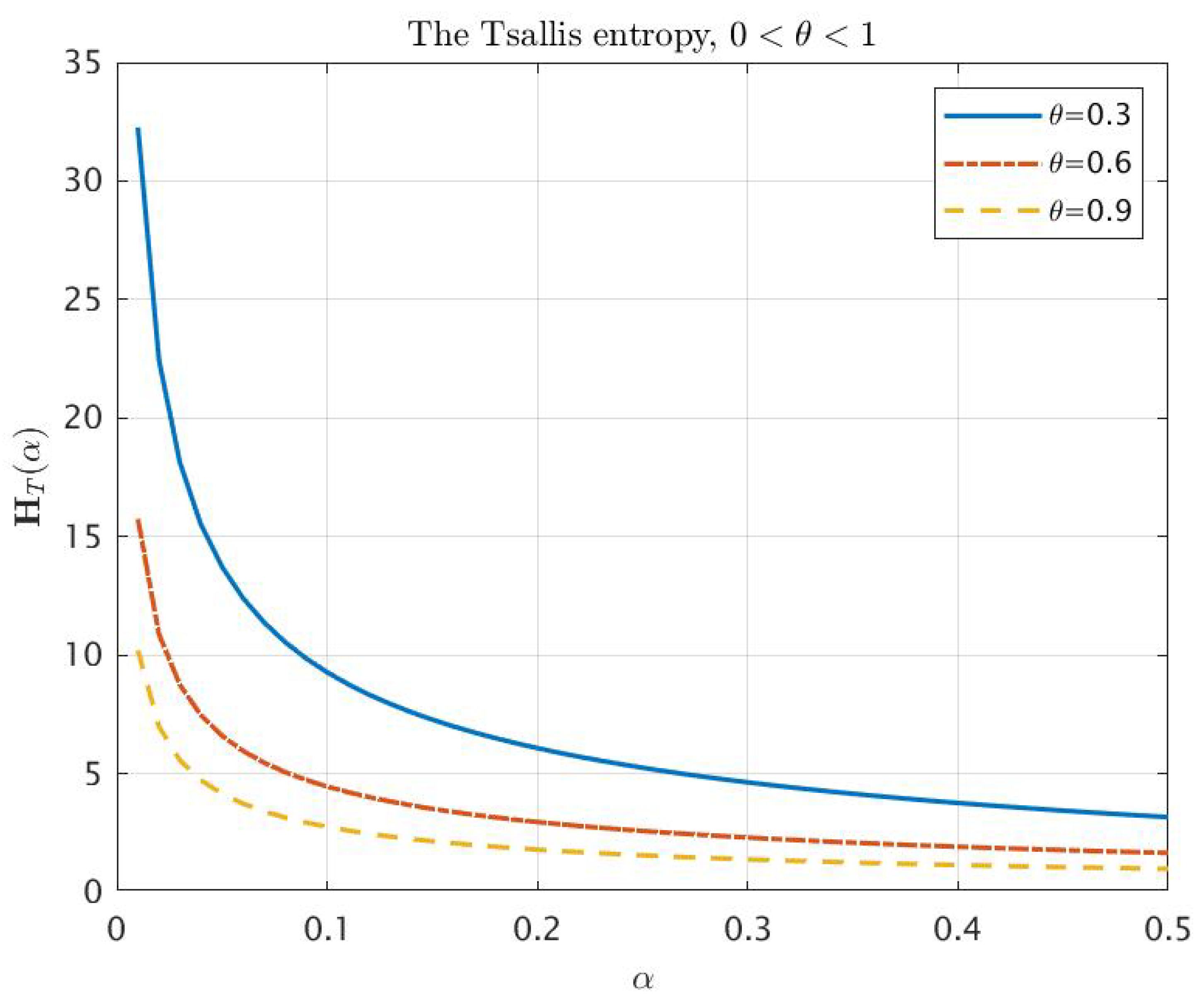
Figure 1 and Figure 2 correspond to the behavior of Tsallis entropy for θ < 1 . Two cases need to be investigated numerically:
θ ( 1 , e x 0 ) , α > x 0 log θ
and
θ > e x 0 , α < x 0 log θ .
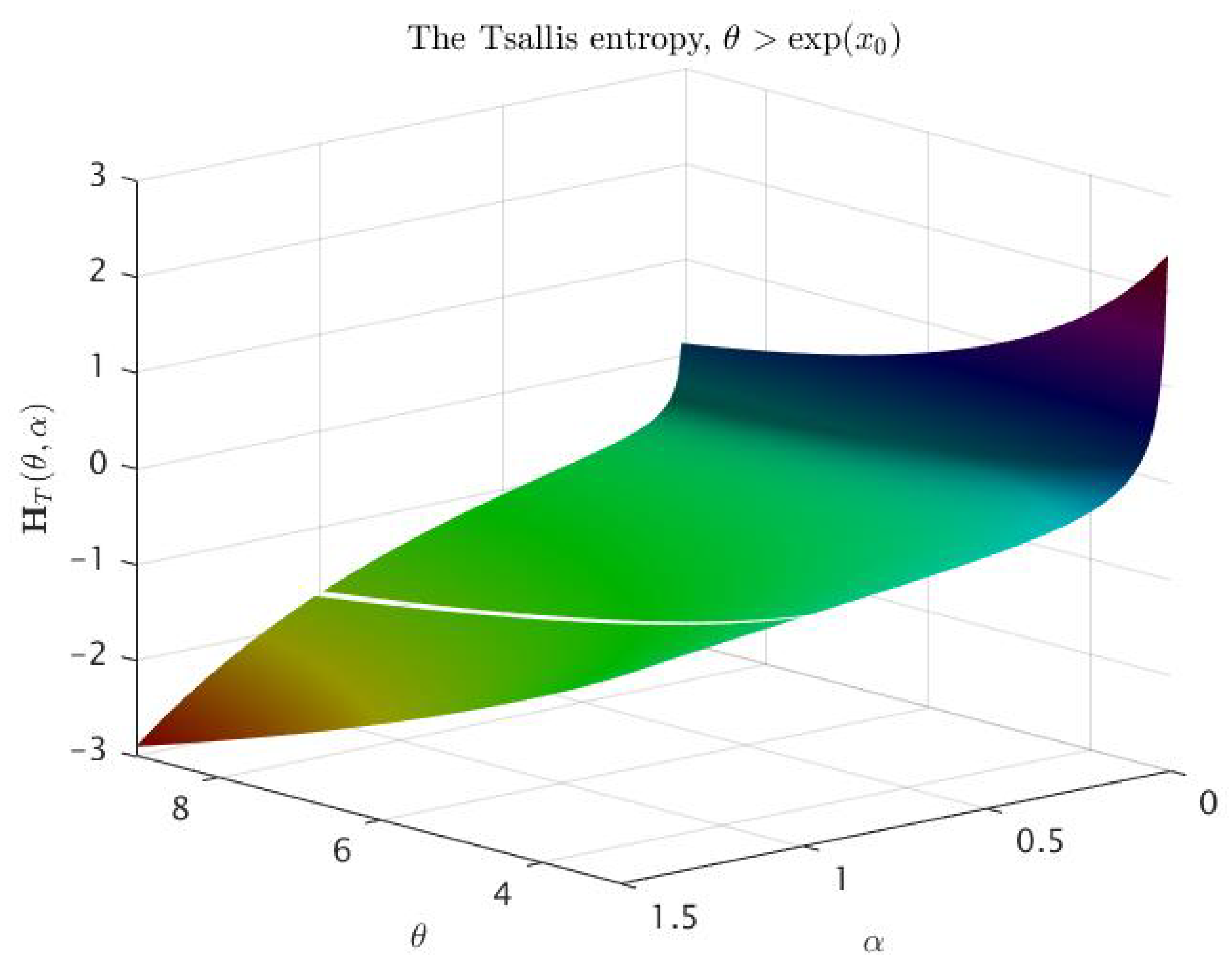
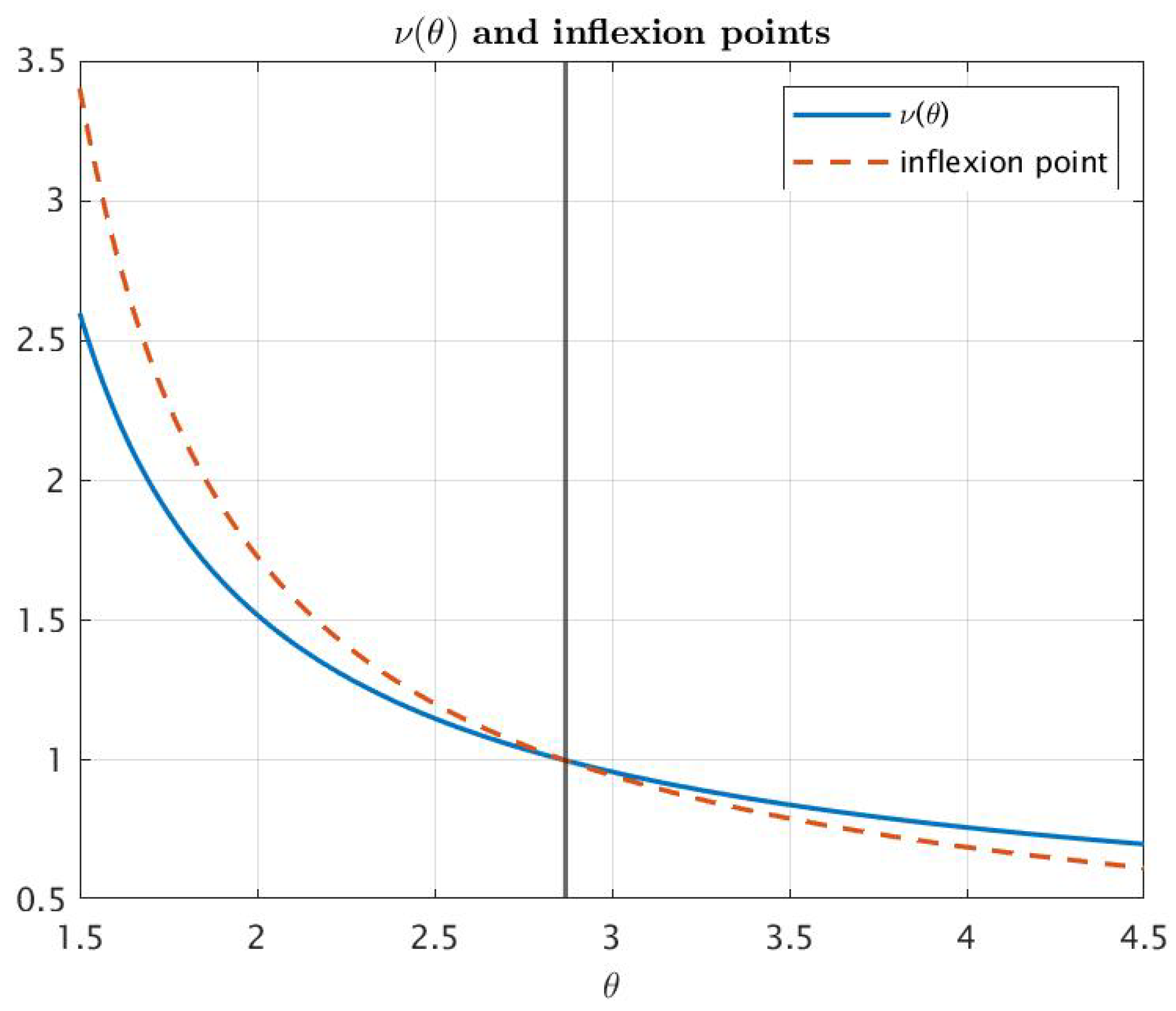
In both cases, we already know from item ( d ) of Theorem 3 that H T is a convex function on the interval ( 0 , α ( 1 , θ ) ) and is a concave function on the interval ( α ( 2 , θ ) , ) for some 0 < α ( 1 , θ ) < α ( 2 , θ ) < . The surfaces plotted on Figure 3 and Figure 4 confirm numerically that for any θ > 1 , there exists the unique inflection point α ( 0 , θ ) ( α ( 1 , θ ) , α ( 2 , θ ) ) of H T as the function of α. Furthermore, Figure 5 and Figure 6 give us an idea of the entropy graphs for different θ. The marked points are points of the intersection of the entropy graph with the vertical line ν ( θ ) = x 0 log θ . Note that e x 0 2.86788 ; therefore, the values of θ in Figure 5 correspond to the interval ( 1 , e x 0 ) , while the values in Figure 6 correspond to ( e x 0 , ) .
Moreover, we numerically compared the values of the inflection points which are the solutions of the equation H T ( α ) = 0 (which is equivalent to 1 2 g ( α ) ( α 1 ) 2 g ( α ) ( α 1 ) + g ( α ) 1 = 0 ; see (7)) with ν ( θ ) . Figure 7 confirms that the unique inflection point is close to ν ( θ ) , slightly overcomes ν ( θ ) for θ < e x 0 and is less than ν ( θ ) for θ > e x 0 . In the case θ = e x 0 , we have a coincidence of inflection points with ν ( θ ) = 1 .
Now, let us study the properties of the Sharma–Mittal entropy H S M ( α , β ) as the function of parameters α and β . It is well known (see [21]) that the Shannon, Rényi and Tsallis entropies are the limiting cases of H S M ( α , β ) , namely
H S M ( α , β ) H R ( α ) as β 1 , H S M ( α , β ) H T ( α ) as β α , H S M ( α , β ) H S as α , β 1 .
Therefore, the Sharma–Mittal entropy can be extended to a continuous function of α and β .
Theorem 4.
Consider, as before, the centered normal distribution with variance σ 2 .
(1) 
Let us denote
θ 1 = θ 1 ( α ) = 2 π σ α 1 2 ( 1 α ) .
For any fixed α > 0 , α 1 , H S M ( α , β ) decreases in β ( 0 , + ) , namely as follows:
(i) 
If θ 1 = 1 , then H S M ( α , β ) = 0 .
(ii) 
If θ 1 < 1 , then H S M ( α , β ) decreases from θ 1 1 to .
(iii) 
If θ 1 > 1 , then H S M ( α , β ) decreases from θ 1 1 to 0.
(b) 
For any fixed α > 0 , α 1 , the function H S M ( α , β ) is concave in β if θ 1 < 1 , and it is convex if θ 1 > 1 .
(b) 
For a fixed β ( 0 , 1 ) ( 1 , ) , H S M ( α , β ) is a decreasing and convex function in α.
Proof. 
(1) We have
H S M ( α , β ) = θ 1 1 β 1 1 β , β ( 0 , 1 ) ( 1 , ) .
Denote x = 1 β ( , 0 ) ( 0 , 1 ) . Then,
F ( x ) = θ 1 x 1 x = θ 1 x θ 1 0 x 0
is a slope function for f ( x ) = θ 1 x , which in convex. Therefore, F ( x ) is increasing in x ( , 0 ) ( 0 , 1 ) . Consequently, the statements (i)(iii) hold.
(2) Let θ 1 < 1 . We can write
H S M ( α , β ) = g 1 ( β ) g 1 ( 1 ) β 1 , β ( 0 , 1 ) ( 1 , ) .
where g 1 ( β ) = θ 1 1 β . Since the third derivative g 1 ( β ) = θ 1 1 β ( log θ 1 ) 3 is positive for θ 1 < 1 , we see that H S M ( α , β ) is convex in β by Lemma A1 from Appendix B. Hence, H S M ( α , β ) is concave in β .
In the case θ 1 > 1 , we represent H S M ( α , β ) in the following form:
H S M ( α , β ) = g 2 ( β ) g 2 ( 1 ) β 1 , β ( 0 , 1 ) ( 1 , ) ,
where g 2 ( β ) = g 1 ( β ) = θ 1 1 β . For θ 1 > 1 , we have g 2 ( β ) = θ 1 1 β ( log θ 1 ) 3 > 0 ; hence, the desired convexity follows from Lemma A1.
(3) It is not hard to see that
log θ 1 ( α ) = H R ( α ) ,
where H R ( α ) is the Rényi entropy, which is a decreasing function of α according to Theorem 1. Hence, θ 1 ( α ) decreases. Moreover,
α H S M ( α , β ) = θ 1 ( α ) θ 1 β ( α ) < 0 ,
and H S M ( α , β ) also decreases in α .
In order to establish convexity, we differentiate (8) and obtain θ 1 ( α ) θ 1 ( α ) = H R ( α ) , whence θ 1 ( α ) = θ 1 ( α ) H R ( α ) and
θ 1 ( α ) = θ 1 ( α ) H R ( α ) + θ 1 ( α ) H R ( α ) > 0 ,
because θ 1 ( α ) < 0 , H R ( α ) < 0 , and H R ( α ) > 0 , according to Theorem 1 and to the previous statement. Then, by differentiation of (9), we obtain
2 α 2 H S M ( α , β ) = θ 1 ( α ) θ 1 β ( α ) β θ 1 β 1 ( α ) θ 1 ( α ) θ 1 2 β ( α ) > 0 ,
since θ 1 ( α ) > 0 and θ 1 ( α ) < 0 . Thus, convexity is proved.  □
Remark 5.
Let us consider the equation θ 1 = 1 , i.e.,
α 1 2 ( 1 α ) = 2 π σ
or
log α 2 ( 1 α ) = log 2 π σ = : ρ .
According to the proof of Theorem 1 (statement 3), the function log α 2 ( 1 α ) increases from to 0 in α ( 0 , 1 ) ( 1 , ) .
Thus:
  • If 2 π σ > 1 , then θ 1 > 1 and (iii) holds.
  • If 2 π σ = 1 , then (iii) holds too.
  • If 2 π σ < 1 , then let α 0 be a number such that
    α 0 1 2 ( 1 α 0 ) = 2 π σ .
    If α < α 0 , then θ 1 > 1 and (iii) holds. If α > α 0 , then θ 1 < 1 and (ii) holds. If α = α 0 , then θ 1 = 1 and (i) holds.

3. Examples of Gaussian Fractional Processes with Their Variances: Entropies of Fractional Gaussian Processes

Now, we consider several types of fractional Gaussian processes. Our goal is very simple: to compare the entropies of their marginal distributions. In order to compare their entropies and variances correctly, we normalize the variances using the normalizing coefficients so that at the point t = 1 , the variance of every process equals 1.
As already mentioned in the introduction, the entropy of vector fractional Gaussian noise is calculated using the formulas given in the book [23]. However, firstly, these calculations are based on the fact that fractional Gaussian noise is a stationary process, and secondly, using them to compare different processes, even fractional Gaussian noise with different Hurst indices, is too complicated a problem for an analytical solution. The main difficulty is that the formula for the entropy of a Gaussian vector contains the determinant of the covariance matrix, the calculation of which there are no simple proposals for at the moment, except for cumbersome standard formulas, and at the same time, they do not make it possible to compare these determinants. Therefore, having at our disposal several classes of fractional processes that model a wide variety of processes, from physics to financial mathematics, we set out to compare in as simple a way as possible the terms of the information they carry, or, more simply, to compare their entropies. The comparisons of entropies presented are based on calculating the variances of the corresponding processes, and these calculations are quite simple and understandable to a wide range of readers.

3.1. Fractional, Subfractional and Bifractional Brownian Motions

Let us start with the definition of fractional Brownian motion. This process was first introduced in [25].
Definition 2.
A centered Gaussian process B H = { B t H , t 0 } with a covariance function
Cov B t H , B s H = 1 2 t 2 H + s 2 H | t s | 2 H , t , s R +
is called a fractional Brownian motion (fBm) with the Hurst parameter H ( 0 , 1 ) .
Obviously, Var ( B t H ) = t 2 H .
Definition 3
([26]). A centered Gaussian process ξ H = { ξ t H , t 0 } with a covariance function
Cov ξ t H , ξ s H = s 2 H + t 2 H 1 2 ( s + t ) 2 H + | t s | 2 H , t , s 0
is called a subfractional Brownian motion with the Hurst parameter H ( 0 , 1 )
Obviously,
Var ξ t H = 2 t 2 H 1 2 ( 2 t ) 2 H = 2 2 2 H 1 t 2 H .
Let us put ξ ¯ t H = ( 2 2 2 H 1 ) 1 2 ξ t H . Then, ξ ¯ t H has the same variance as fractional Brownian motion.
Definition 4
([27] (p.71)). The process L H = { L t H , t 0 } , defined by
L t H = 1 Γ ( H + 1 2 ) 0 t ( t s ) H 1 / 2 d W s , t 0 , H ( 0 , 1 ) ,
and where W = { W t , t 0 } is a Wiener process, is called a Riemann–Liouville fractional Brownian motion.
Then
Var ( L t H ) = 1 Γ 2 ( H + 1 2 ) 0 t ( t u ) 2 H 1 d u = t 2 H 2 H Γ 2 ( H + 1 2 ) .
Therefore, the process L ¯ H = ( 2 H ) 1 / 2 Γ ( H + 1 2 ) L t H has the same variance as fractional Brownian motion and subfractional Brownian motion.
Definition 5
([28]). A centered Gaussian process B H , K = { B t H , K , t 0 } , starting from zero, with a covariance function
Cov B t H , K , B s H , K : = 1 2 K ( t 2 H + s 2 H ) K | t s | 2 H K
is called a bifractional Brownian motion with H ( 0 , 1 ) and K ( 0 , 1 ] .
Then
Var B t H , K = Cov B t H , K , B t H , K = 1 2 K ( t 2 H + t 2 H ) K = t 2 H K .
Obviously, at point t = 1 , variance equals Var ( B 1 H , K ) = 1 .
Proposition 2.
Let X be one of the following processes: B H , ξ ¯ H or L ¯ H . Then, one has the following formulas for the entropies of X t :
(1) 
The Shannon entropy equals
H S X ( t ) = H log t + 1 2 ( 1 + log ( 2 π ) ) .
(2) 
The Rényi entropy ( α > 0 , α 1 ) equals
H R X ( α , t ) = H log t + 1 2 log ( 2 π ) + log α 2 ( α 1 ) .
For α = 1 , we extend the Rényi entropy by the Shannon entropy continuously.
(3) 
The generalized Rényi entropy in the case α = β equals
H G R X ( α , t ) = H log t + 1 2 log ( 2 π ) + 1 2 α ,
and for α = β = 1 , we extend the generalized Rényi entropy by the Shannon entropy (and Rényi entropy with α = 1 ) continuously.
(4) 
The generalized Rényi entropy in the case α β equals
H G R X ( α , β , t ) = H log t + 1 2 log ( 2 π ) + log β log α 2 ( β α ) ,
and for α = β , it can be extended by the generalized Rényi entropy in the case α = β continuously.
(5) 
The Tsallis entropy ( α > 0 , α 1 ) equals
H T X ( α , t ) = t ( 1 α ) H ( 2 π ) 1 α 2 α 1 / 2 1 1 α ,
and for α = 1 , it can be extended by the Shannon entropy continuously.
(6) 
The Sharma–Mittal entropy for α , β ( 0 , 1 ) ( 1 , ) equals
H S M X ( α , β , t ) = 1 1 β t ( 1 β ) H ( 2 π ) 1 β 2 α 1 β 2 ( 1 α ) 1 ,
and for β = 1 , it can be extended by the Rényi entropy continuously.
(7) 
The same statements hold for X = B H , K with H K instead of H. This means that any entropy of bifractional Brownian motion with parameters H and K equals to the corresponding entropy of fBm with Hurst index H = H K . In turn, this means that if we fix the same H in fBm and bifractional Brownian motion and take K < 1 , then
H A B H ( · , t ) < H A B H , K ( · , t ) , t < 1 ,
A = S , R , G R , and opposite inequality holds for t > 1 . For H T X ( α , t ) , the situation is more involved: if t < 1 , α < 1 or t > 1 , α > 1 , then
H T B H ( α , t ) < H T B H , K ( α , t ) ,
and for t < 1 , α > 1 or t > 1 , α < 1 , the opposite inequality holds.
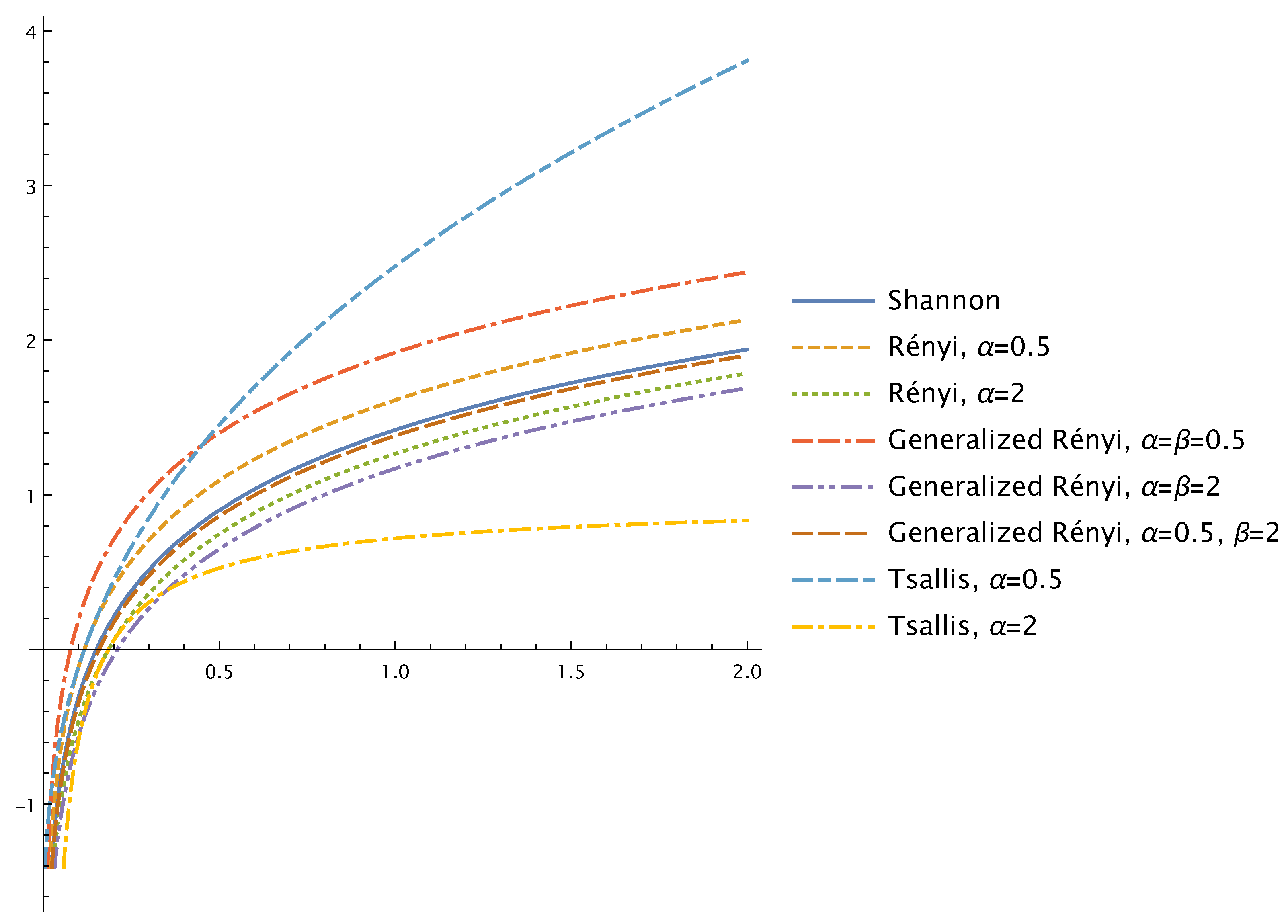
Figure 8 contains graphs of various entropies of fractional Brownian motion with Hurst parameter H = 0.75 .
Remark 6.
It is interesting and natural to compare the variance of fBm B H = { B t H , t 0 } with the variance of the corresponding fractional Ornstein–Uhlenbeck process X t H = 0 t e α ( t s ) d B s H for various H and α and consequently to compare their entropies. Consider the following cases.
( i ) Let H > 1 2 . Then, according to [29],
Var X t H = 2 H ( 2 H 1 ) 0 t 0 t e α ( 2 t s u ) | s u | 2 H 2 d u d s .
If α > 0 , then e α ( 2 t s u ) > 1 , and
Var X t H > 2 H ( 2 H 1 ) 0 t 0 t | s u | 2 H 2 d u d s = Var B t H .
Similarly, if α < 0 , then Var X t H < Var B t H .
( i i ) Let H < 1 2 . Then, the integral is understood via integration by parts [30]:
X t H = B t H + α 0 t e α ( t s ) B s H d s .
Let α > 0 . Then,
Var X t H = Var B t H + 2 α 0 t e α ( t s ) E B t H B s H d s + α 2 0 t 0 t e α ( 2 t s u ) E B s H B u H d u d s > Var B t H ,
because E [ B s H B u H ] = 1 2 ( s 2 H + u 2 H | u s | 2 H ) > 0 and similarly E [ B t H B s H ] > 0 .
Let α < 0 . Denote β = α > 0 . Then, our goal is to determine the sign of the value
θ ( t ) : = 2 β 0 t e β ( t s ) E B t H B s H d s + β 2 0 t 0 t e β ( 2 t s u ) E B s H B u H d u d s .
Now, we change the variables β s = r , β u = q and take into account that E [ B t / β H B s / β H ] = β 2 H E [ B t H B s H ] , and similarly, E [ B s / β H B u / β H ] = β 2 H E [ B s H B u H ] , denote β t = z and also take into account the symmetry of the integrand in the 2nd integral and, with all of this at hand, arrive at the value
φ ( z ) = 0 z e z + r z 2 H + r 2 H ( z r ) 2 H d r + 0 z 0 r e 2 z + r + q r 2 H + q 2 H ( r q ) 2 H d q d r ,
whose sign is interesting for us. Obviously,
φ ( z ) = z 2 H e z e z 1 e z 0 z e r r 2 H d r + 0 z e v v 2 H d v + e 2 z 0 z e r r 2 H e r 1 d r + e 2 z 0 z e r 0 r e q q 2 H d q d r e 2 z 0 z e 2 r 0 r e v v 2 H d v d r .
Equivalently, we can consider the sign of function
ψ ( z ) = e 2 z φ ( z ) = z 2 H e 2 z e z e z 0 z e r r 2 H d r + e 2 z 0 z e v v 2 H d v + 0 z e r r 2 H e r 1 d r + 0 z e r 0 r e q q 2 H d q d r 0 z e 2 r 0 r e v v 2 H d v d r .
Obviously, ψ ( 0 ) = 0 . Furthermore,
ψ ( z ) = 2 H z 2 H 1 e 2 z e z z 2 H 2 e 2 z e z e z 0 z e r r 2 H d r e 2 z z 2 H + 2 e 2 z 0 z e v v 2 H d v + e z z 2 H + e z z 2 H e z 1 + e z 0 z e q q 2 H d q e 2 z 0 z e v v 2 H d v = 2 H z 2 H 1 e 2 z e z 2 z 2 H e 2 z + z 2 H e z e 2 z z 2 H + 2 e 2 z 0 z e v v 2 H d v + e z z 2 H + e 2 z z 2 H e z z 2 H e 2 z 0 z e v v 2 H d v = 2 H z 2 H 1 e 2 z e z 2 z 2 H e 2 z + z 2 H e z + e 2 z 0 z e v v 2 H d v < 2 H z 2 H 1 e 2 z e z 2 z 2 H e 2 z + z 2 H e z + e 2 z z 2 H 1 e z = 2 H z 2 H 1 e 2 z e z z 2 H e 2 z < 0 .
This means that ψ ( z ) < 0 for all z > 0 ; consequently, θ ( t ) < 0 for all t > 0 . Together with (16), this finally means that Var X t H > Var B t H if α > 0 , and Var X t H < Var B t H if α < 0 .
Remark 7.
Note that fractional Ornstein–Uhlenbeck process was generalized in the papers [31,32] to the massive-FBM and the diffusing–diffusivity-FBM. The diffusing–diffusivity-FBM is non-Gaussian, but the massive-FBM can be considered in the framework of fractional Ornstein–Uhlenbeck processes, and the calculations above can help in the comparison of the entropies.

3.2. Multifractional Brownian Motion

Let us consider various definitions of multifractional Brownian motion. The difference is in the form of their representation; the same situation that we have with standard fBm: it admits Mandelbrot–van Ness representation [33] on the whole axis, Molchan–Golosov compact interval representation [29] and spectral representation (Section 7.2.2 of [34]). However, covariance and variance functions of all fBms are the same and can differ only by normalizing multipliers (correct values of the multipliers are provided, for example, in [35]). Considering different representations of multifractional Brownian motion, the authors introduce different normalizing multipliers, basically following the form of this factor for the corresponding representation of fractional Brownian motion, but in this case, they depend on time. Below, we provide these representations and analyze the relations between them and the behavior of the normalizing multipliers as the functions on time, because their value influences the value of variance and consequently the value of the entropy. Obviously, if we renormalize the processes in order to equate their variances, the entropies become equal.
Let H : R + [ a , b ] ( 0 , 1 ) be a continuous function.
Definition 6
([36]). For t 0 , the following random function is called moving-average multifractional Brownian motion with functional parameter H:
Y 1 ( t ) = 1 Γ ( H t + 1 2 ) 0 [ ( t s ) H t 1 / 2 ( s ) H t 1 / 2 ] d W ( s ) + 0 t ( t s ) H t 1 / 2 d W ( s ) = 1 Γ ( H t + 1 2 ) t [ ( t s ) H t 1 / 2 ( s ) + H t 1 / 2 ] d W ( s ) ,
where W denotes the Brownian motion.
It follows from Cor. 3.4 of [33] that
Var [ Y 1 ( t ) ] = c 1 ( H t ) t 2 H t ,
where
c 1 ( x ) = 1 Γ ( x + 1 2 ) 2 0 ( 1 s ) x 1 2 ( s ) x 1 2 2 d s + 1 2 H , x ( 0 , 1 ) .
The function c 1 ( x ) can be written in the following form Appendix A of [35]:
c 1 ( x ) = 1 2 x Γ ( 2 x ) sin ( π x ) .
Let us consider the process Y ¯ 1 ( t ) = Y 1 ( t ) c 1 ( H 1 ) . Then,
Var [ Y ¯ 1 ( t ) ] = c 1 ( H t ) c 1 ( H 1 ) t 2 H t , Var [ Y ¯ 1 ( 1 ) ] = 1 .
Remark 8.
The coefficient 1 Γ ( H t + 1 ) in (17) goes back to the seminal work of Mandelbrot and van Ness [33], who defined fractional Brownian motion as a fractional integral of the Wiener process (this factor ensures that a fractional integral becomes an ordinary repeated integral for integer values of H t 1 2 ). However, in the literature, the moving-average multifractional Brownian motion is often defined with a different normalizing constant, namely, it is defined as Y ˜ 1 ( t ) = Y 1 ( t ) c 1 ( H t ) . In this case, we obviously have that Var Y ˜ 1 ( t ) = t 2 H t .
Let us consider a different type of multifractional Brownian motion, introduced in [37,38]. It is based on the Molchan–Golosov compact interval representation of fBm [29]. Note that in the next definition, the class of appropriate Hurst functions is restricted to the case H t > 1 2 .
Definition 7
([37]). Let H : R + ( 1 2 , 1 ) . For t 0 , the following random function is called Volterra-type multifractional Brownian motion with functional parameter H:
Y 2 ( t ) = 0 t s 1 / 2 H t s t u H t 1 / 2 ( u s ) H t 3 / 2 d u d W ( s ) ,
where W denotes the Brownian motion.
Then, by Prop. 2 of [37],
Var [ Y 2 ( t ) ] = c 2 ( H t ) t 2 H t ,
where
c 2 ( x ) = Γ ( 2 2 x ) Γ ( x 1 2 ) 2 sin ( π ( x 1 2 ) ) 2 π x ( x 1 2 ) , x ( 1 / 2 , 1 ) .
Hence, the process Y ¯ 2 ( t ) = Y 2 ( t ) c 2 ( H 1 ) has the variance
Var [ Y ¯ 2 ( t ) ] = c 2 ( H t ) c 2 ( H 1 ) t 2 H t
and Var [ Y ¯ 2 ( 1 ) ] = 1 .
Remark 9.
In [38], the authors defined the Volterra-type multifractional Brownian motion with a normalizing function in front of the integral, i.e., by the relation Y ˜ 2 ( t ) = Y 2 ( t ) c 2 ( H t ) . Evidently, in this case, one has Var Y ˜ 2 ( t ) = t 2 H t .
Definition 8
([39]). The harmonizable multifractional Brownian motion with functional parameter H is defined by
Y 3 ( t ) = R e i t u 1 | u | H t + 1 / 2 d W ( u ) , t 0 .
where W ˜ ( d u ) is the “Fourier transform” of the white noise W ( d u ) that is a unique complex-valued random measure such that for all f L 2 ( R )
R f ( u ) W ( d u ) = R f ^ ( u ) W ˜ ( d u ) a . s . ;
see [39,40].
It is known from Prop. 4 of [41] that
Var [ Y 3 ( t ) ] = c 3 ( H t ) t 2 H t ,
where
c 3 ( x ) = π x Γ ( 2 x ) sin ( π x ) .
Define the normalized version of the harmonizable multifractional Brownian motion by Y ¯ 3 ( t ) = Y 3 ( t ) c 3 ( H 1 ) so that
Var [ Y ¯ 3 ( t ) ] = c 3 ( H t ) c 3 ( H 1 ) t 2 H t and Var [ Y ¯ 3 ( 1 ) ] = 1 .
Proposition 3.
One has the following formulas for the entropies of Y ¯ i ( t ) , i = 1 , 2 , 3 .
(1) 
The Shannon entropy equals
H S Y ¯ i ( t ) = H t log t + 1 2 log c i ( H t ) 1 2 log c i ( H 1 ) + 1 2 ( 1 + log ( 2 π ) ) .
(2) 
The Rényi entropy ( α > 0 , α 1 ) equals
H R Y ¯ i ( α , t ) = H t log t + 1 2 log c i ( H t ) 1 2 log c i ( H 1 ) + 1 2 log ( 2 π ) + log α 2 ( α 1 ) .
(3) 
The generalized Rényi entropy in the case α = β equals
H G R Y ¯ i ( α , t ) = H t log t + 1 2 log c i ( H t ) 1 2 log c i ( H 1 ) + 1 2 log ( 2 π ) + 1 2 α .
(4) 
The generalized Rényi entropy in the case α β equals
H G R Y ¯ i ( α , β , t ) = H t log t + 1 2 log c i ( H t ) 1 2 log c i ( H 1 ) + 1 2 log ( 2 π ) + log β log α 2 ( β α ) .
(5) 
The Tsallis entropy ( α > 0 , α 1 ) equals
H T Y ¯ i ( α , t ) = t ( 1 α ) H t ( 2 π c i ( H t ) / c i ( H 1 ) ) 1 α 2 α 1 / 2 1 1 α .
(6) 
The Sharma–Mittal entropy for α , β ( 0 , 1 ) ( 1 , ) equals
H S M Y ¯ i ( α , β , t ) = 1 1 β t ( 1 β ) H t ( 2 π c i ( H t ) / c i ( H 1 ) ) 1 β 2 α 1 β 2 ( 1 α ) 1 .
Now, let us compare entropies for various versions of multifractional Brownian motion. Recall that the Volterra-type multifractional Brownian motion Y 2 is well-defined only for H t > 1 2 .
Proposition 4.
Let H : R + ( 0 , 1 ) and A = S , R , G R , T , S M .
(1) 
For all t 0 , H A Y ¯ 1 ( · , t ) = H A Y ¯ 3 ( · , t ) .
(2) 
Let H t > 1 2 . Then
H A Y ¯ 1 ( · , t ) H A Y ¯ 2 ( · , t ) if H t H 1 , H A Y ¯ 1 ( · , t ) H A Y ¯ 2 ( · , t ) if H t H 1 .
Proof. 
( i ) It follows immediately from (18) and (21) that c 3 ( x ) c 1 ( x ) = 2 π for all x ( 0 , 1 ) . This means that for any Hurst function H t ,
Var [ Y ¯ 1 ( t ) ] = c 1 ( H t ) c 1 ( H 1 ) t 2 H t = c 3 ( H t ) c 3 ( H 1 ) t 2 H t = Var [ Y ¯ 3 ( t ) ] ,
i.e., the entropies for Y 1 ( t ) and Y 3 ( t ) coincide.
( i i ) According to Remark 1, all entropies are increasing functions of the variance. Therefore, it suffices to compare the variances of moving-average and Volterra-type multifractional Brownian motions.
For x ( 1 2 , 1 ) , Formulas (18) and (19) imply that
c 2 ( x ) c 1 ( x ) = Γ ( 2 x ) Γ ( 2 2 x ) Γ ( x 1 2 ) 2 sin ( π ( x 1 2 ) ) sin ( π x ) π ( x 1 2 ) = 2 Γ ( 2 x 1 ) Γ ( 2 2 x ) Γ ( x 1 2 ) 2 sin ( π ( x 1 2 ) ) sin ( π x ) π = 2 sin ( π ( x 1 2 ) ) sin ( π x ) sin ( π ( 2 x 1 ) ) Γ ( x 1 2 ) 2 = Γ ( x 1 2 ) 2 .
Hence,
Var Y ¯ 2 ( t ) Var Y ¯ 1 ( t ) = Γ ( H t 1 2 ) 2 Γ ( H 1 1 2 ) 2 .
Since the function Γ ( x 1 2 ) decreases for x ( 1 2 , 1 ) , we see that Var Y ¯ 1 ( t ) Var Y ¯ 2 ( t ) if and only if H t H 1 .  □

3.3. Tempered Fractional Brownian Motion

Two classes of continuous stochastic Gaussian processes, known as tempered fractional Brownian motion (TFBM) and tempered fractional Brownian motion of the second kind (TFBMII), were recently introduced in [42] and [43], respectively. These processes modify the power law kernel used in the moving-average representation of fBm by introducing exponential tempering. Unlike standard fBm, TFBMs can be defined for any Hurst parameter value H > 0 . These processes attracted the attention of researchers in various fields. Notably, a stochastic phenomenological bifurcation of the Langevin equation perturbed by TFBM was constructed in [44], revealing diverse and intriguing bifurcation phenomena. Additionally, TFBM and TFBMII are valuable as stochastic models for data exhibiting fractional Brownian motion characteristics at intermediate scales but deviating at longer scales, such as wind speed measurements.
Definition 9.
Given an independently scattered Gaussian random measure W ( d x ) on R with control measure dx, for any H > 0 and λ > 0 , the stochastic process B H , λ I = { B H , λ I ( t ) , t 0 } defined by the Wiener integral
B H , λ I ( t ) : = t e λ ( t x ) ( t x ) H 1 / 2 e λ ( x ) + ( x ) + H 1 / 2 W ( d x ) ,
where 0 0 = 0 is called a tempered fractional Brownian motion (TFBM).
Since TFBM ([45] (p. 7)) has the covariance function
Cov B H , λ I ( t ) , B H , λ I ( s ) = 1 2 ( C t I ) 2 t 2 H + ( C s I ) 2 s 2 H ( C | t s | I ) 2 | t s | 2 H
for any s , t R , where
( C t I ) 2 = 2 Γ ( 2 H ) ( 2 λ t ) 2 H 2 Γ ( H + 1 / 2 ) π 1 ( 2 λ t ) H K H ( λ t ) ,
where t 0 and K ν ( z ) is the modified Bessel function of the second kind (see Appendix C), then we have
Var ( B H , λ I ( t ) ) = ( C t I ) 2 t 2 H .
Definition 10.
Given an independently scattered Gaussian random measure W ( d x ) on R with control measure dx, for any H > 0 and λ > 0 , the stochastic process B H , λ I I = { B H , λ I I ( t ) , t 0 } defined by the Wiener integral
B H , λ I I ( t ) : = t g H , λ , t I I ( x ) W ( d x ) ,
where
g H , λ , t I I ( x ) : = ( t x ) H 1 / 2 e λ ( t x ) ( x ) + H 1 / 2 e λ ( x ) + + λ 0 t ( s x ) + H 1 / 2 e λ ( s x ) + d s , x R .
is called a tempered fractional Brownian motion of the second kind (TFBMII).
According to [45] (p. 7), TFBMII has the covariance function
Cov ( B H , λ I I ( t ) , B H , λ I I ( s ) ) = 1 2 ( C t I I ) 2 t 2 H + ( C s I I ) 2 s 2 H ( C | t s | I I ) 2 | t s | 2 H
for any s , t R , where
( C t I I ) 2 = ( 1 2 H ) Γ ( H + 1 / 2 ) Γ ( H ) ( λ t ) 2 H π × 1 2 F 3 ( { 1 , 1 / 2 } , { 1 H , 1 / 2 , 1 } , λ 2 t 2 / 4 ) + Γ ( 1 H ) Γ ( H + 1 / 2 ) π H 2 2 H 2 F 3 ( { 1 , H 1 / 2 } , { 1 , H + 1 , H + 1 / 2 } , λ 2 t 2 / 4 ) ,
and 2 F 3 is the generalized hypergeometric function, defined in Appendix C. Therefore, the value of the correspondent variance equals
Var ( B H , λ I I ( t ) ) = ( C t I I ) 2 t 2 H .
Let us define
B ¯ H , λ I ( t ) = B H , λ I ( t ) C 1 I , B ¯ H , λ I I ( t ) = B H , λ I I ( t ) C 1 I I .
Then,
Var [ B ¯ H , λ I ( t ) ] = ( C t I ) 2 ( C 1 I ) 2 t 2 H , Var [ B ¯ H , λ I I ( t ) ] = ( C t I I ) 2 ( C 1 I I ) 2 t 2 H ,
and Var [ B ¯ H , λ I ( 1 ) ] = Var [ B ¯ H , λ I I ( 1 ) ] = 1 .
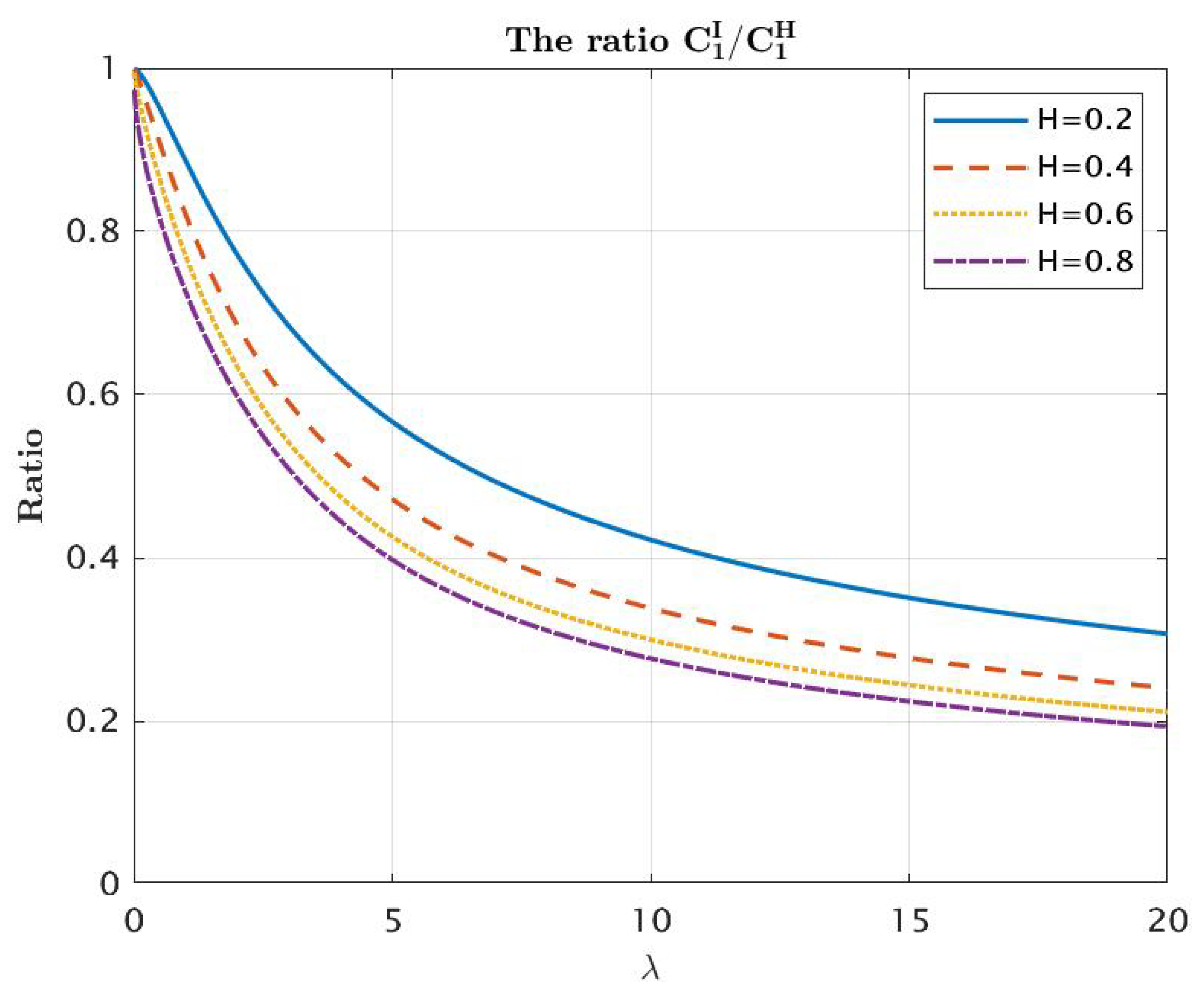
According to Remark 1, in order to compare the entropies of B ¯ H , λ I ( t ) and B ¯ H , λ I I ( t ) , it suffices to compare their variances. By (30), this problem can be reduced to the investigation of the behavior of the ratio C t I / C t I I . Namely, we need to compare its value at arbitrary point t to its value at t = 1 . Note also that the dependence of C t I and C t I I on λ is such that C t I ( λ ) = C 1 I ( λ t ) , C t I I ( λ ) = C 1 I I ( λ t ) . Therefore, it suffices to study the ratio C 1 I / C 1 I I as a function of λ . As it may be seen from Figure 9, this ratio decreases in λ for all selected values of H. Thus, our numerical study leads to the following conjecture:
Var B ¯ H , λ I ( t ) > Var B ¯ H , λ I I ( t ) if t < 1
and
Var B ¯ H , λ I ( t ) < Var B ¯ H , λ I I ( t ) if t > 1 .
The analytical proof of this result is challenging due to the complexity of expressions (28) and (29).
Remark 10.
For the reader’s convenience, the MATLAB scripts for the figures are published as Supplementary Material.

4. Conclusions

We examined five distinct entropy measures applied to the Gaussian distribution: Shannon entropy, Rényi entropy, generalized Rényi entropy, Tsallis entropy and Sharma–Mittal entropy. We investigated their interrelationships and analyzed their properties in terms of their dependence on specific parameters. Furthermore, our study extends to fractional Gaussian processes, encompassing fractional Brownian motion, subfractional Brownian motion, bifractional Brownian motion, multifractional Brownian motion and tempered fractional Brownian motion. We conducted a comparative analysis of the entropies associated with the one-dimensional distributions of these processes.
Entropy measures find widespread application in the analysis of fractional processes across various domains, such as signal processing, finance, climate science and image analysis. Fractional processes serve as essential models for capturing long-range dependence and self-similarity in diverse data types. Entropy plays a crucial role in quantifying the complexity and information content of signals generated by fractional processes, which proves invaluable for tasks like prediction, risk assessment and anomaly detection. In the realm of finance, entropy is employed to assess the information content and predictability of asset prices.
Our research opens up possibilities for future extensions in several directions. Potential avenues for further investigation include exploring various entropy measures for non-Gaussian processes, nonstationary processes and processes with nonstationary increments. Additionally, we can delve into the solutions of stochastic differential equations that describe the interactions of particle systems within random environments.

Supplementary Materials

The following supporting information can be downloaded at https://www.mdpi.com/article/10.3390/axioms12111026/s1, the MATLAB scripts for the figures.

Author Contributions

Investigation, A.M., Y.M., K.R. and Y.A.R.; writing—original draft preparation, A.M., Y.M., K.R. and Y.A.R. All authors have read and agreed to the published version of the manuscript.

Funding

The second author is supported by The Swedish Foundation for Strategic Research, grant Nr. UKR22-0017 and by Japan Science and Technology Agency CREST, project reference number JPMJCR2115. The third author acknowledges that the present research is carried out within the frame and support of the ToppForsk project nr. 274410 of the Research Council of Norway with title STORM: Stochastics for Time-Space Risk Models.

Data Availability Statement

No new data were created or analyzed in this study. Data sharing is not applicable to this article.

Conflicts of Interest

The authors declare no conflict of interest.

Appendix A. Computation of Entropies for Centered Normal Distribution

Appendix A.1. Shannon Entropy

The following transformations are obvious:
H S = R f ( x ) log f ( x ) d x = R 1 σ 2 π exp x 2 2 σ 2 log 1 σ 2 π exp x 2 2 σ 2 d x = R exp x 2 2 σ 2 σ 2 π log 1 σ 2 π x 2 2 σ 2 d x = log 1 σ 2 π + R 1 σ 2 π exp x 2 2 σ 2 x 2 2 σ 2 d x = log σ 2 π + 1 / 2 = 1 / 2 ( 1 + log 2 π ) + log σ .

Appendix A.2. Rényi Entropy

R f α ( x ) d x = R 1 σ 2 π exp x 2 2 σ 2 α d x = 1 σ 2 π α R exp x 2 α 2 σ 2 d x = 1 σ 2 π α 2 π σ 2 / α 2 π σ 2 / α R exp x 2 2 ( σ / α ) 2 d x = 1 σ 2 π α 2 π σ α = 1 σ α 1 ( 2 π ) α 1 2 α 1 / 2 ,
whence
H R ( α ) = 1 1 α log R f α ( x ) d x = 1 α 1 log σ α 1 ( 2 π ) α 1 2 α 1 / 2 = log σ + 1 / 2 log ( 2 π ) + log α 2 ( α 1 ) .

Appendix A.3. Generalized Rényi Entropy

Let us calculate the generalized Rényi entropy in the case α = β . We denote γ : = σ α and use Formula (A1):
H G R ( α ) = R f α ( x ) log f ( x ) d x R f α ( x ) d x = R δ α e α x 2 2 σ 2 log δ + x 2 2 σ 2 d x · δ α 1 α 1 / 2 = δ α 1 / 2 δ α R 1 γ 2 π e x 2 2 γ 2 log δ + x 2 2 σ 2 d x · δ α 1 α 1 / 2 = log δ + 1 2 σ 2 R x 2 e x 2 2 γ 2 1 γ 2 π d x = log δ + 1 2 σ 2 γ 2 = log δ + 1 2 α .
To calculate the generalized Rényi entropy in the case α β , we use Formula (A1):
H G R ( α , β ) = 1 β α log R f α ( x ) d x R f β ( x ) d x = 1 β α log δ β 1 β δ α 1 α = 1 β α log δ β α β / α = log δ + log β log α 2 ( β α ) .

Appendix A.4. Tsallis Entropy

The Tsallis entropy ( α > 0 , α 1 ) can be calculated using Formula (A1) as follows:
H T ( α ) = 1 1 α R f α ( x ) d x 1 = 1 δ α 1 α 1 / 2 1 1 α = δ 1 α α 1 / 2 1 1 α .

Appendix A.5. Sharma–Mittal Entropy

The Sharma–Mittal entropy ( α > 0 , α 1 , β 1 ) is calculated similarly. By (A1), we have
H S M ( α , β ) = 1 1 β R f α ( x ) d x 1 β 1 α 1 = 1 1 β 1 σ α 1 ( 2 π ) α 1 2 α 1 / 2 1 β 1 α 1 = 1 1 β ( 2 π σ ) 1 β α 1 β 2 ( 1 α ) 1 .

Appendix B. Auxiliary Lemma

Lemma A1.
Let function g C ( 3 ) ( 0 , + ) and g ( x ) > 0 , x > 0 , x 0 > 0 . Then, the function
ψ ( x ) = g ( x ) g ( x 0 ) x x 0 , x > 0
is convex.
Proof. 
Let us calculate the derivatives:
ψ ( x ) = g ( x ) ( x x 0 ) g ( x ) + g ( x 0 ) ( x x 0 ) 2 ,
ψ ( x ) = g ( x ) ( x x 0 ) 3 2 ( x x 0 ) ( g ( x ) ( x x 0 ) g ( x ) + g ( x 0 ) ) ( x x 0 ) 4 = 2 g ( x ) g ( x 0 ) g ( x ) ( x x 0 ) + 1 2 g ( x ) ( x x 0 ) 2 ( x x 0 ) 3 = 2 g ( x ) g ( x 0 ) + g ( x ) ( x 0 x ) + 1 2 g ( x ) ( x 0 x ) 2 ( x x 0 ) 3 .
According to the Taylor formula,
g ( x 0 ) = g ( x ) + g ( x ) ( x 0 x ) + 1 2 g ( x ) ( x 0 x ) 2 + 1 6 g ( ξ ) ( x 0 x ) 3 ,
where ξ is between x and x 0 , i.e., ξ [ x x 0 , x x 0 ] .
Therefore,
g ( x ) g ( x 0 ) + g ( x ) ( x 0 x ) + 1 2 g ( x ) ( x 0 x ) 2 = 1 6 g ( ξ ) ( x 0 x ) 3
Finally,
ψ ( x ) = 2 1 6 g ( ξ ) ( x 0 x ) 3 ( x x 0 ) 3 = 1 3 g ( ξ ) > 0 .
Consequently, the function ψ ( x ) is convex.  □

Appendix C. Special Functions Kν and 2F3

In this subsection, we present definitions of two special functions, K ν and 2 F 3 , which we used in Section 3.3.
A modified Bessel function of the second kind  K ν ( x ) has the integral representation
K ν ( x ) = 0 e x cosh t cosh ν t d t ,
where ν > 0 , x > 0 . The function K ν ( x ) also has the series representation
K ν ( x ) = 1 2 π I ν ( x ) I ν ( x ) sin ( π ν ) ,
where I ν ( x ) = ( 1 2 | x | ) ν n = 0 ( 1 2 x ) 2 n n ! Γ ( n + 1 + ν ) is called the Bessel function. We refer the reader to Section 8.43 of [46] for more information about the modified Bessel function of the second kind.
Next, we define the confluent hypergeometric function  2 F 3 that we used to obtain the variance and covariance of TFBMII. In general, a generalized hypergeometric function p F q is defined by
p F q ( a 1 , , a p , b 1 , , b q , z ) = k = 0 ( a 1 ) k ( a 2 ) k ( a p ) k ( b 1 ) k ( b 2 ) k ( b q ) k z k k ! ,
where ( c i ) k = Γ ( c i + k ) Γ ( k ) is called Pochhammer Symbol. Therefore,
2 F 3 ( { a 1 , a 2 } , { b 1 , b 2 , b 3 } , z ) = 2 F 3 ( a 1 , a 2 , b 1 , b 2 , b 3 , z ) = k = 0 Γ ( a 1 + k ) Γ ( a 2 + k ) Γ ( k ) Γ ( b 1 + k ) Γ ( b 2 + k ) Γ ( b 3 + k ) z k k ! .

References

  1. Shannon, C.E. A mathematical theory of communication. Bell Syst. Tech. J. 1948, 27, 379–423. [Google Scholar] [CrossRef]
  2. Cover, T.M.; Thomas, J.A. Elements of Information Theory; Wiley: Hoboken, NJ, USA, 2006. [Google Scholar]
  3. Quinlan, J.R. Induction of decision trees. Mach. Learn. 1986, 1, 81–106. [Google Scholar] [CrossRef]
  4. Pathria, R.K. Statistical Mechanics; Elsevier: Amsterdam, The Netherlands, 2011. [Google Scholar]
  5. Schneier, B. Applied Cryptography: Protocols, Algorithms, and Source Code in C; Wiley: Hoboken, NJ, USA, 1996. [Google Scholar]
  6. Nei, M.; Tajima, F. DNA polymorphism detectable by restriction endonucleases. Genetics 1981, 97, 145–163. [Google Scholar] [CrossRef]
  7. Brock, W.; Lakonishok, J.; LeBaron, B. Simple technical trading rules and the stochastic properties of stock returns. J. Financ. 1992, 47, 1731–1764. [Google Scholar] [CrossRef]
  8. Lorenz, E.N. Deterministic nonperiodic flow. J. Atmos. Sci. 1963, 20, 130–141. [Google Scholar] [CrossRef]
  9. Wasserman, S.; Faust, K. Social Network Analysis: Methods and Applications; Cambridge University Press: Cambridge, UK, 1994. [Google Scholar]
  10. Mullet, E.; Karakus, M. A cross-cultural investigation of the triarchic model of well-being in Turkey and the United States. J. Cross-Cult. Psychol. 2006, 37, 141–149. [Google Scholar]
  11. Nielsen, M.A.; Chuang, I.L. Quantum Computation and Quantum Information; Cambridge University Press: Cambridge, UK, 2000. [Google Scholar]
  12. Rahman, A.U.; Haddadi, S.; Javed, M.; Kenfack, L.T.; Ullah, A. Entanglement witness and linear entropy in an open system influenced by FG noise. Quantum Inf. Process. 2022, 21, 368. [Google Scholar] [CrossRef]
  13. Li, K.; Zhou, W.; Yu, S.; Dai, B. Effective DDoS Attacks Detection Using Generalized Entropy Metric. In Proceedings of the Algorithms and Architectures for Parallel Processing; 9th International Conference, ICA3PP 2009, Taipei, Taiwan, 8–11 June 2009; Hua, A., Chang, S.L., Eds.; Springer: Berlin/Heidelberg, Germany, 2009; pp. 266–280. [Google Scholar]
  14. Morabito, F.C.; Labate, D.; Foresta, F.L.; Bramanti, A.; Morabito, G.; Palamara, I. Multivariate multi-scale permutation entropy for complexity analysis of Alzheimer’s disease EEG. Entropy 2012, 14, 1186–1202. [Google Scholar] [CrossRef]
  15. Wu, Y.; Chen, P.; Luo, X.; Wu, M.; Liao, L.; Yang, S.; Rangayyan, R.M. Measuring signal fluctuations in gait rhythm time series of patients with Parkinson’s disease using entropy parameters. Biomed. Signal Process. Control 2017, 31, 265–271. [Google Scholar] [CrossRef]
  16. Rényi, A. On measures of entropy and information. In Proceedings of the 4th Berkeley Symposium on Mathematical Statistics and Probability, Vol. I, Berkeley, CA, USA, 20 June–30 July 1960; University California Press: Berkeley, CA, USA; Los Angeles, CA, USA, 1960; pp. 547–561. [Google Scholar]
  17. Tsallis, C. Possible generalization of Boltzmann-Gibbs statistics. J. Stat. Phys. 1988, 52, 479–487. [Google Scholar] [CrossRef]
  18. Tsallis, C. The nonadditive entropy Sq and its applications in physics and elsewhere: Some remarks. Entropy 2011, 13, 1765–1804. [Google Scholar] [CrossRef]
  19. Sharma, B.D.; Taneja, I.J. Entropy of type (α, β) and other generalized measures in information theory. Metrika 1975, 22, 205–215. [Google Scholar] [CrossRef]
  20. Sharma, B.D.; Mittal, D.P. New non-additive measures of relative information. J. Combin. Inform. Syst. Sci. 1977, 2, 122–132. [Google Scholar]
  21. Nielsen, F.; Nock, R. A closed-form expression for the Sharma–Mittal entropy of exponential families. J. Phys. A 2012, 45, 032003. [Google Scholar] [CrossRef]
  22. Buryak, F.; Mishura, Y. Convexity and robustness of the Rényi entropy. Mod. Stoch. Theory Appl. 2021, 8, 387–412. [Google Scholar] [CrossRef]
  23. Stratonovich, R.L. Theory of Information and Its Value; Springer: Cham, Switzerland, 2020. [Google Scholar]
  24. Malyarenko, A.; Mishura, Y.; Ralchenko, K.; Shklyar, S. Entropy and alternative entropy functionals of fractional Gaussian noise as the functions of Hurst index. Fract. Calc. Appl. Anal. 2023, 26, 1052–1081. [Google Scholar] [CrossRef]
  25. Kolmogorov, A.N. Wienersche Spiralen und einige andere interessante Kurven im Hilbertschen Raum. Dokl. Acad. Sci. USSR 1940, 26, 115–118. [Google Scholar]
  26. Bojdecki, T.; Gorostiza, L.G.; Talarczyk, A. Sub-fractional Brownian motion and its relation to occupation times. Statist. Probab. Lett. 2004, 69, 405–419. [Google Scholar] [CrossRef]
  27. Mishura, Y.; Zili, M. Stochastic Analysis of Mixed Fractional Gaussian Processes; ISTE Press: London, UK; Elsevier Ltd.: Oxford, UK, 2018. [Google Scholar]
  28. Russo, F.; Tudor, C.A. On bifractional Brownian motion. Stoch. Process. Appl. 2006, 116, 830–856. [Google Scholar] [CrossRef]
  29. Norros, I.; Valkeila, E.; Virtamo, J. An elementary approach to a Girsanov formula and other analytical results on fractional Brownian motions. Bernoulli 1999, 5, 571–587. [Google Scholar] [CrossRef]
  30. Cheridito, P.; Kawaguchi, H.; Maejima, M. Fractional Ornstein–Uhlenbeck processes. Electron. J. Probab. 2003, 8, 1–14. [Google Scholar] [CrossRef]
  31. Cherstvy, A.G.; Wang, W.; Metzler, R.; Sokolov, I.M. Inertia triggers nonergodicity of fractional Brownian motion. Phys. Rev. E 2021, 104, 024115. [Google Scholar] [CrossRef]
  32. Wang, W.; Seno, F.; Sokolov, I.M.; Chechkin, A.V.; Metzler, R. Unexpected crossovers in correlated random-diffusivity processes. New J. Phys. 2020, 22, 083041. [Google Scholar] [CrossRef]
  33. Mandelbrot, B.B.; Van Ness, J.W. Fractional Brownian motions, fractional noises and applications. SIAM Rev. 1968, 10, 422–437. [Google Scholar] [CrossRef]
  34. Samorodnitsky, G.; Taqqu, M.S. Stable Non-Gaussian Random Processes; Chapman & Hall: New York, NY, USA, 1994. [Google Scholar]
  35. Mishura, Y.S. Stochastic Calculus for Fractional Brownian Motion and Related Processes; Lecture Notes in Mathematics; Springer-Verlag: Berlin, Germany, 2008; Volume 1929. [Google Scholar]
  36. Peltier, R.F.; Lévy Véhel, J. Multifractional Brownian Motion: Definition and Preliminary Results; [Research Report] RR-2645; INRIA: Le Chesnay, France, 1995. [Google Scholar]
  37. Boufoussi, B.; Dozzi, M.; Marty, R. Local time and Tanaka formula for a Volterra-type multifractional Gaussian process. Bernoulli 2010, 16, 1294–1311. [Google Scholar] [CrossRef]
  38. Ralchenko, K.; Shevchenko, G. Properties of the paths of a multifractal Brownian motion. Theory Probab. Math. Statist. 2010, 80, 119–130. [Google Scholar] [CrossRef]
  39. Benassi, A.; Jaffard, S.; Roux, D. Elliptic Gaussian random processes. Rev. Mat. Iberoam. 1997, 13, 19–90. [Google Scholar] [CrossRef]
  40. Stoev, S.A.; Taqqu, M.S. How rich is the class of multifractional Brownian motions? Stoch. Process. Appl. 2006, 116, 200–221. [Google Scholar] [CrossRef]
  41. Ayache, A.; Cohen, S.; Lévy Véhel, J. The covariance structure of multifractional Brownian motion, with application to long range dependence. In Proceedings of the 2000 IEEE International Conference on Acoustics, Speech, and Signal Processing. Proceedings (Cat. No. 00CH37100), Istanbul, Turkey, 5–9 June 2000; Volume 6, pp. 3810–3813. [Google Scholar]
  42. Meerschaert, M.M.; Sabzikar, F. Tempered fractional Brownian motion. Statist. Probab. Lett. 2013, 83, 2269–2275. [Google Scholar] [CrossRef]
  43. Sabzikar, F.; Surgailis, D. Tempered fractional Brownian and stable motions of second kind. Statist. Probab. Lett. 2018, 132, 17–27. [Google Scholar] [CrossRef]
  44. Zeng, C.; Yang, Q.; Chen, Y. Bifurcation dynamics of the tempered fractional Langevin equation. Chaos 2016, 26, 084310. [Google Scholar] [CrossRef]
  45. Azmoodeh, E.; Mishura, Y.; Sabzikar, F. How does tempering affect the local and global properties of fractional Brownian motion? J. Theoret. Probab. 2022, 35, 484–527. [Google Scholar] [CrossRef]
  46. Gradshteyn, I.S.; Ryzhik, I.M. Table of Integrals, Series, and Products; Academic Press: New York, NY, USA, 2020. [Google Scholar]
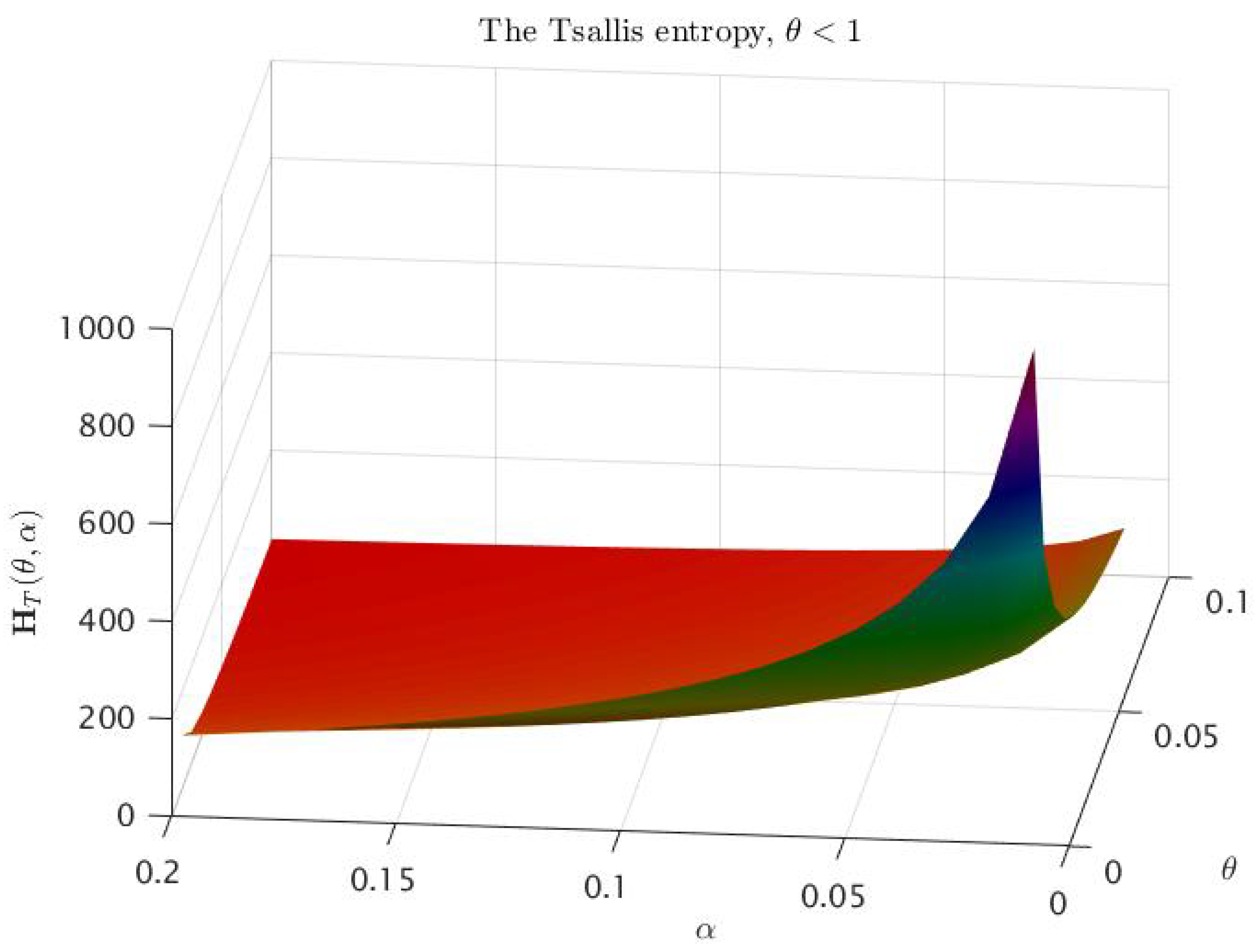
Figure 1. Tsallis entropy as a function of θ and α , θ < 1 .
Axioms 12 01026 g001
Figure 2. Tsallis entropy as a function of α for θ = 0.3 , 0.6 , 0.9 .
Axioms 12 01026 g002
Figure 3. Tsallis entropy as a function of θ and α , 1 < θ < e x 0 .
Axioms 12 01026 g003
Figure 4. Tsallis entropy as a function of θ and α , θ > e x 0 .
Axioms 12 01026 g004
Figure 5. Tsallis entropy as a function of α for θ = 1.5 , 2.0 , 2.8 .
Axioms 12 01026 g005
Figure 6. Tsallis entropy as a function of α for θ = 3 , 5 , 9 .
Axioms 12 01026 g006
Figure 7. ν ( θ ) and inflection points.
Axioms 12 01026 g007
Figure 8. Various entropies of fractional Brownian motion with Hurst parameter H = 0.75 as functions of t.
Axioms 12 01026 g008
Figure 9. The ratio C 1 I / C 1 I I as a function of λ .
Axioms 12 01026 g009
Disclaimer/Publisher’s Note: The statements, opinions and data contained in all publications are solely those of the individual author(s) and contributor(s) and not of MDPI and/or the editor(s). MDPI and/or the editor(s) disclaim responsibility for any injury to people or property resulting from any ideas, methods, instructions or products referred to in the content.