A Novel Robust Topological Denoising Method Based on Homotopy Theory for Virtual Colonoscopy

Abstract

Virtual colonoscopy plays an important role in polyp detection of colorectal cancer. Noise in the colon data acquisition process can result in topological errors during surface reconstruction. Topological denoising can be employed to remove these errors on surfaces for subsequent geometry processing, such as surface simplification and parameterization. Many methods have been proposed for this task. However, many existing methods suffer from failure in computation of all the non-trivial loops, due to high genus or complex topological structures. In this paper, we propose a novel robust topological denoising method for surfaces based on homotopy theory. The proposed method was evaluated on two datasets of colon meshes. We compared our method with the State-of-the-Art persistent-homology-based method. Our method can successfully compute the loops on all colon data for topological denoising, whereas the persistent homology method fails on some colon data. Moreover, our method detects all loops with shorter lengths than those detected by the persistent homology method. Our experimental results show that the proposed method is effective and robust in topological denoising, and that it has the potential for practical application to virtual colonoscopy.

1. Introduction

In the medical imaging field, virtual colonoscopy (VC) plays an important role in detecting polyps for colorectal cancer. Studies use CT images and various computerized methods to assist in the detection of polyps. Methods based on topographical height map [1], polyp-specific volumetric feature [2], ensemble learning [3], morphological features [4], and integration with optical colonoscopy [5] have been explored in the field. Some other studies have focused on the improvement of VC by using an immersive analytics system [6] and a deep learning framework [7,8]. A recent study also investigated the feasibility of the automated detection of clinically significant polyps from photon-counting CT data [9]. One of the representative forms of colon data is based on colon surface mesh, which is reconstructed from computed tomography (CT) scans. Such surface-based colon data processing methods highly depend on the quality of the reconstructed colon surface, such that it is without topological noises or errors. With the rapid advances in data acquisition techniques in recent decades, high resolution of three-dimensional data has been produced for various applications, including real-time vision processing [10], industrial application [11], textured 3D mesh generation [12], blood flow simulation [13], cardiac structure reconstruction [14], robotic 3D reconstruction of an object [15], ceramics analysis and reconstruction [16], and unmanned-aerial-vehicles-based 3D reconstruction [17], etc. However, many existing surface reconstruction methods introduce topological noises or errors into the resulting reconstructed surfaces, which makes it intractable to perform subsequent computation tasks, such as surface simplification and parameterization.

As one important geometry processing technique, topological denoising aims to decrease or remove topological noises, usually in the form of small handle loops, so that a lower-genus or genus-zero resulting model can be generated. Success in the topological denoising process significantly rests on the efficient computation of those non-trivial loops, followed by robust genus reduction, such as cutting along the loops. In regard to computation of non-trivial loops on surfaces, we have witnessed a variety of methods in recent decades. Some of these methods are based on homotopy and homology [18,19,20], and some are based on graph structures, such as curve skeletons [21], core graph [22,23], and Reeb graph [24].

Chen et al. [19] proposed a method to compute loops using persistent homology. The method employed the greedy algorithm, to compute the optimal homology basis. Dey et al. [20] presented a geometry-aware method, to compute handle and tunnel loops, which aimed to balance computation between topological correct loops and geometrically relevant loops. They applied the proposed method to topology simplification and to handle and tunnels feature identification. In addition to these methods based on homology, researchers have proposed graph-based methods. Zhou et al. [21] introduced a loop detection algorithm, using skeletons based on the medial axis for topological denoising or repair. The advantages of this method are: (1) it will not introduce additional invalid handles; (2) it can process large surface models with high resolutions, efficiently. However, this method cannot be used in models whose medial axis forms closed surfaces. Dey et al. [22,23] designed a handle and tunnel loop computation method on graph retractable surfaces, which employed a linking condition with the core graphs. They demonstrated the effectiveness of their method by applying it to feature detection and topology simplification. Later, Dey et al. [24] utilized Reeb graphs to compute handle and tunnel loops. Their method is computationally efficient, without requiring any 3D tessellation. More recently, Weinrauch et al. [25] proposed a variational abstraction to the loop shrinking property for detection of handle and tunnel loops. Their method utilizes a succinct diffuse interface model for loop detection and a fully parallel algorithmic realization. However, some limitations exist in these methods, which lie in either non-guaranteed computation of non-trivial loops, in terms of some geometrically meaningful requirements, or even failure in the computation of all the non-trivial loops, due to very high genus or complex topological structures.

In recent decades, topological denoising has attracted wide attention from the medical community. In cardiac image analysis, where the trabeculae structure is naturally a topological handle, Gao et al. [26] used persistent homology to localize the trabeculae. Wu et al. [27] formulated the computation of the optimal cycles of persistent homology classes for trabeculae detection. These methods can be applied for better understanding the functionality of the human heart and for diagnosing cardiac diseases. In biotechnology, Brezovsky et al. [28] reviewed some tools for identification of the protein tunnels and channels, as it is important to understand the relationship between structure and function and to design potential proteins that have improved functional properties. A tool named CHUNNEL can be used to identify the loop running around the narrowest part of the protein channel. Topologically denoised 3D data can be flattened to a 2D domain for supplementary information or views [29,30,31,32,33,34,35,36,37,38]. In virtual colonoscopy, flattening the 3D colon wall surface into a 2D domain, via surface parameterization, not only benefits visualization—which assists in detection of abnormality, such as colorectal polyps—but also enables the computation of supplementary geometric and texture features in the 2D flattened colon wall, for improved computer-aided detection of polyps. One important pre-processing step is to perform topological denoising on the original 3D colon wall surface, so that the small handle loops on the surface are removed, to obtain a genus-zero surface for subsequent colon wall flattening. To this end, some existing works [35,37,39] have employed the homotopy-based topological denoising method for genus reduction, followed by surface flattening using conformal parameterization. Although the existing methods are capable of computing the small handle loops in the colon wall and performing topological denoising to reduce the genus of the surface, it is still challenging, but desirable, to obtain a robust topological denoising method.

In this work, we propose a novel robust topological denoising method for virtual colonoscopy. The algorithm is detailed in some steps involving computations of cut graph, shortest loops, and topological surgery. Experiments on two datasets were carried out, for evaluation of the proposed method. The main contributions in this paper are as follows:

(1)

Mathematical rigor. Our proposed method is based on rigorous mathematical theory in homotopy, which guarantees the computation of the non-trivial loops.

(2)

Novel framework. The proposed algorithm is novel and has been first applied to colon surface denoising in virtual colonoscopy.

(3)

Robust computation. Compared to the State-of-the-Art topological denoising method, our method is more robust, based on the experimental results.

2. Materials and Methods

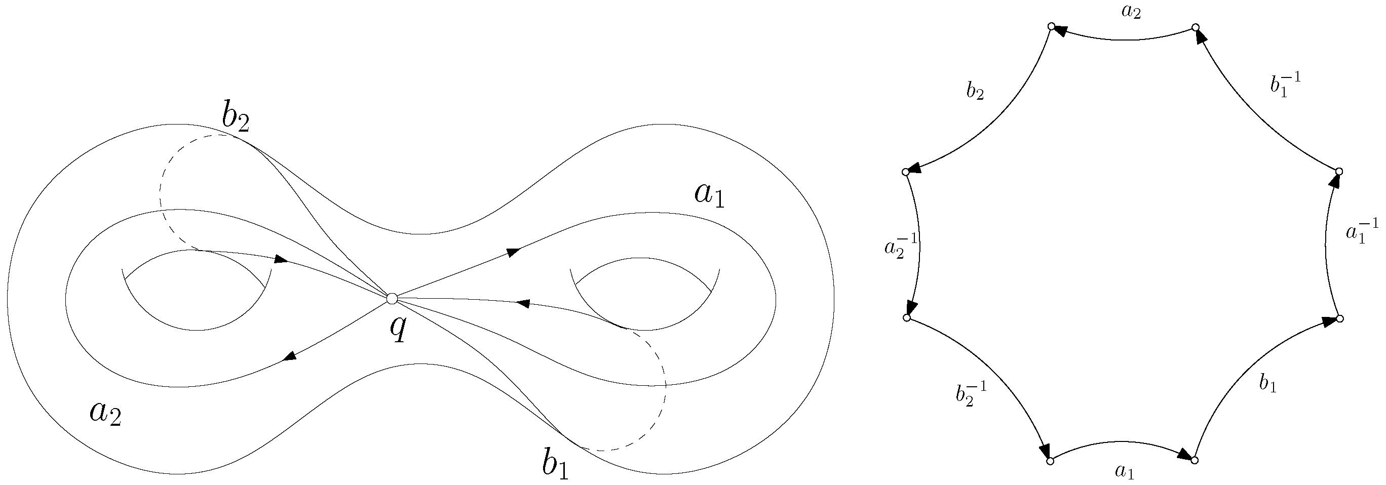
2.1. Theoretic Background

This section briefly explains the basic concepts and theorems in algebraic topology. For more thorough treatments, we refer readers to a classical algebraic textbook [40].

Suppose S is a topological surface, and a path is a continuous map $\gamma :[0,1]\to S$; if the starting point coincides with the ending point, $\gamma \left(0\right)=\gamma \left(1\right)$, then $\gamma$ is a closed curve (loop).

Definition 1 (Homotopy).

Let ${\gamma }_1,{\gamma }_2:[0,1]\to S$ be two curves. A homotopy connecting ${\gamma }_1$ and ${\gamma }_2$ is a continuous mapping $F:[0,1]\times [0,1]\to S$, such that

$$F(0,t)={\gamma }_1\left(t\right),F(1,t)={\gamma }_2\left(t\right).$$

(1)

We say ${\gamma }_1$ is homotopic to ${\gamma }_2$ if there exists a homotopy between them, and we denote it as ${\gamma }_1\sim {\gamma }_2$.

Homotopy relation is an equivalence relation. We fix a base point p on the surface. In the following, we consider all the loops through the base point, denoted as $\Gamma$. All the loops in $\Gamma$ can be classified by the homotopy equivalence relation, and the homotopy class of $\gamma \in \Gamma$ is denoted as $\left[\gamma \right]$.

Given two loops ${\gamma }_1,{\gamma }_2\in \Gamma$ through the base point p, we can concatenate them to form a bigger loop, which is the product of the two loops, denoted as ${\gamma }_1·{\gamma }_2$. There is a special loop e for all $t\in [0,1]$, $e\left(t\right)=p$, which is called the trivial loop. It is evident that $e·\gamma =\gamma ·\gamma =\gamma$ for any loop $\gamma$. Suppose $\gamma \in \Gamma$ is a loop on S, then its inverse is obtained by reversing the orientation ${\gamma }^{-1}\in \Gamma$, ${\gamma }^{-1}\left(t\right)=\gamma (1-t)$. It is easy to verify that $\gamma ·{\gamma }^{-1}\sim e$ and ${\gamma }^{-1}·\gamma \sim e$. All the homotopy classes of $\Gamma$ under the product operator form a group.

Definition 2 (Fundamental Group).

Given a topological space S, fix a base point $p\in S$; the set of all the loops through p is Γ, and the set of all the homotopy classes is $\Gamma /\sim$. The product is defined as

$$\left[{\gamma }_1\right]·\left[{\gamma }_2\right]:=[{\gamma }_1·{\gamma }_2],$$

(2)

the unit element is defined as $\left[e\right]$, and the inverse element is defined as

$${\left[\gamma \right]}^{-1}:=\left[{\gamma }^{-1}\right];$$

(3)

then, $\Gamma /\sim$ forms a group, the fundamental group of S, and is denoted as ${\pi }_1(S,p)$.

In the following, we show the generators and relators of the fundamental group ${\pi }_1(S,p)$. Suppose S is an oriented closed surface, then the number of handles of S is called the genus of the surface. Suppose ${\gamma }_1\left(t\right),{\gamma }_2\left(\tau \right)\subset S$ intersect at $q\in S$, the tangent vectors satisfy

$$\frac{d{\gamma }_1\left(t\right)}{dt}\times \frac{d{\gamma }_2\left(\tau \right)}{d\tau }·\mathbf{n}\left(q\right)>0;$$

(4)

then, the index of the intersection point q of ${\gamma }_1$ and ${\gamma }_2$ is $+1$, denoted as $\mathrm{Ind}({\gamma }_1,{\gamma }_2,q)=+1$. If the mixed product is zero or negative, then the index is 0 or $-1$.

Definition 3 (Algebraic Intersection Number).

The algebraic intersection number of ${\gamma }_1\left(t\right),{\gamma }_2\left(\tau \right)\subset S$ is defined as

$${\gamma }_1\odot {\gamma }_2:=\sum _{q_i\in {\gamma }_1\cap {\gamma }_2}Ind({\gamma }_1,{\gamma }_2,q_i).$$

(5)

Definition 4 (Canonical Basis).

Suppose S is a compact and oriented surface, then there exists a set of generators of the fundamental group ${\pi }_1(S,p)$,

$$G=\{\left[a_1\right],\left[b_1\right],\left[a_2\right],\left[b_2\right],\dots ,\left[a_g\right],\left[b_g\right]\},$$

(6)

such that

$$a_i\odot b_j={\delta }_i^j,a_i\odot a_j=0,b_i\odot b_j=0,$$

(7)

where $a_i\odot b_j$ represents the algebraic intersection number of loops $a_i$ and $b_j$, and where ${\delta }_{ij}$ is the Kronecker symbol; then, G is called a set of the canonical basis of ${\pi }_1(S,p)$.

Figure 1 shows a genus-2-oriented compact surface S, through the base point $q\in S$. On each handle, there are two loops, $a_i$ and $b_i$, such that the algebraic intersection number of $a_i$ and $b_i$ is $+1$, that of $a_i$ and $a_j$ is 0, that of $b_i$ and $b_j$ is 0, and that of $a_i$ and $b_j$ on different handles is 0. By deforming each $a_i$ and $b_j$, we can slice the surface to get a topological octagon, and its boundary is

$$a_1{b}_1{a}_1^{-1}{b}_1^{-1}{a}_2{b}_2{a}_2^{-1}{b}_2^{-1}.$$

(8)

The set of loops $\{a_1,b_1,a_2,b_2\}$ is called a canonical basis of ${\pi }_1(S,q)$. The number of handles of a surface is called the genus of the surface. The above observation can be directly generalized to high-genus surfaces.

Theorem 1 (Surface Fundamental Group Canonical Representation).

Suppose S is a compact and oriented surface with genus g, that $q\in S$ is the base point, and that the fundamental group has a canonical representation,

$${\pi }_1(S,p)=\langle a_1,b_1,a_2,b_2,\dots ,a_g,b_g|{\Pi }_{i=1}^g[a_i,b_i]\rangle ,$$

(9)

where the $a_i$ values and the $b_j$ values form a set of canonical basis through q; furthermore,

$$[a_i,b_i]=a_i{b}_i{a}_i^{-1}{b}_i^{-1}.$$

(10)

Suppose a compact surface S is embedded in the three-dimensional Euclidean space ${\mathbb{E}}^3$, and it has the induced Euclidean metric $\mathbf{g}$. Suppose p and q are two points close enough to each other, then there is a unique shortest path $\gamma$ connecting them, which is called the geodesic between them. Given a path $\gamma$, if for any point $\gamma \left(t\right)$ there is a small neighborhood $[t-\epsilon ,t+\epsilon ]$, the restriction of $\gamma$ on it is geodesic, and then $\gamma$ is called a (global) geodesic.

Definition 5 (Exponential Map).

Let $\mathbf{v}\in T_{p}S$ be a tangent vector to the surface at p; there is a unique geodesic ${\gamma }_{\mathbf{v}}$ satisfying ${\gamma }_{\mathbf{v}}\left(0\right)=p$ with initial tangent vector ${\gamma }_{\mathbf{v}}^{\prime }=\mathbf{v}$. The corresponding exponential map is defined by

$${exp}_p\left(\mathbf{v}\right)={\gamma }_{\mathbf{v}}\left(1\right).$$

(11)

Definition 6 (Cut Locus).

Fix a point p in a complete Riemannian surface $(S,\mathbf{g})$, and consider the tangent plane $T_{p}S$. The cut locus of p in the tangent space is defined to be the set of all vectors $\mathbf{v}$ in $T_{p}M$, such that $\gamma \left(t\right)={exp}_p\left(t\mathbf{v}\right)$ is a minimizing geodesic for $t\in [0,1]$ but fails to minimize for $t=1+\epsilon$ for any $\epsilon >0$. The cut locus of p in S is defined to be the image of the cut locus of p in the tangent space under the exponential map at p.

Namely, the cut locus of p in S is the point in the surface where the geodesics starting at p stop being minimized.

Our proposed method is based on the following theorem:

Theorem 2 (Main).

Suppose a smooth surface $(S,\mathbf{g})$ is oriented and compact, $p\in S$ is an arbitrarily chosen base point, and the cut locus of p in S is denoted as $\mathcal{C}$. Suppose $\gamma :[0,1]\to S$ is a non-trivial loop on S, then γ intersects with the cut locus $\mathcal{C}$.

Proof. 

Suppose the cut locus of p in the tangent plane is c, then c is a loop on $T_{p}S$ and the interior of c is a planar simply connected open set, denoted as $\Omega$. The exponential map ${exp}_p:T_{p}S\to S$ restricted on $\Omega$ maps $\Omega$ to $S\backslash \mathcal{C}$. Because the exponential map is diffeomorphic in $\Omega$, $S\backslash \mathcal{C}$ is also simply connected.

If a loop $\gamma \subset S$ has no intersection with the cut locus $\mathcal{C}$, then $\gamma \subset S\backslash \mathcal{C}$. But ${\pi }_1(S\backslash \mathcal{C},p)=\langle e\rangle$, therefore $\gamma$ is trivial, which contradicts the assumption that $\gamma$ is non-trivial. Hence, $\gamma$ must intersect the cut locus.    □

2.2. Overview

The pipeline of the proposed topological denoising method is illustrated in Figure 2. We use a simple genus-2 mesh model for illustration purpose, to show the detected loops using our iterative method in two iterations. For higher-genus colon mesh data where the number of genus $n>2$, the proposed method operates in a similar fashion for n iterations. The algorithm of each step is detailed in the following section.

2.3. Algorithms

In this section, we explain our computational algorithm for topological denoising. The volumetric CT images are segmented using the GraphCut method; then, the colon surface is reconstructed, using the MarchingCube algorithm. Hence, the input surface is represented as a simplicial complex (triangle mesh).

Definition 7 (Simplex).

An n-dimensional simplex $\sigma =[v_0,v_1,\dots ,v_n]$ is defined as the convex hull of its vertices, namely,

$$[v_0,v_1,\dots ,v_n]=\left\{{\lambda }_0{v}_0+{\lambda }_1{v}_1+\dots +{\lambda }_n{v}_n|\sum _{i=0}^n{\lambda }_i=1,{\lambda }_i\ge 0\right\}.$$

(12)

The boundary of a simplex $\sigma$ is a set of lower-dimensional simplices, $\partial \sigma =\partial [v_0,v_1,\dots ,v_n]$$={\sum }_{i=0}^n{(-1)}^i[v_0,\dots ,v_{i-1},v_{i+1},\dots ,v_n]$, where the sign represents the parity of the permutation of the vertices of the simplex, and each lower dimensional simplex is called a face of $\sigma$.

Definition 8 (Simplicial Complex).

A simplicial complex $\mathcal{K}$ is a set of simplices that satisfies the following conditions:

1.

Every face of a simplex from $\mathcal{K}$ is also in $\mathcal{K}$.

2.

The non-empty intersection of any two simplices ${\sigma }_1,{\sigma }_2\in \mathcal{K}$ is a face of both ${\sigma }_1$ and ${\sigma }_2$.

The algorithm has three major stages: (1) compute the cut locus (cut graph); (2) compute the shortest non-trivial loop; (3) topological surgery, to remove a handle.

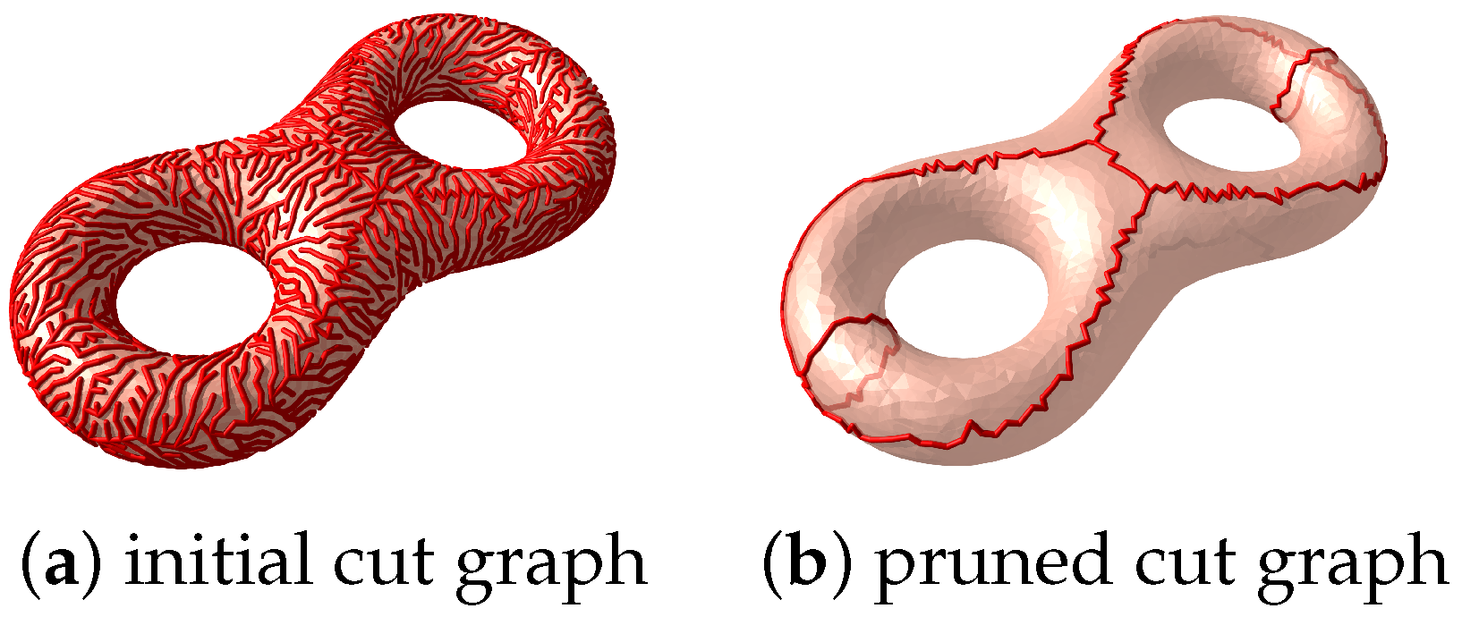
2.3.1. Cut Graph

The cut graph is the analogy of a cut locus on a smooth surface. The computation of the cut graph depends on the construction of the Poincaré dual of the input triangle mesh (as shown in Figure 3), which is the generalization of the duality between the Delaunay triangulation and the Voronoi diagram from plane to manifolds.

In a 2-dimensional (2D) plane setting, as shown in Figure 3, let T be a triangulation of the 2D surface S (i.e., a set of black triangles in the right subfigure), and let $\sigma$ be a simplex of T. A 2D simplex of T containing $\sigma$ is denoted by $\Delta$ (as shown in the left subfigure), and $\sigma$ can be regarded as a subset of the vertices of $\Delta$. The dual cell $\overline{\sigma }$ corresponding to $\sigma$ is defined, such that $\Delta \cap \overline{\sigma }$ (i.e., the gray region in the left subfigure) is the convex hull in $\Delta$ of the barycentres of all subsets of the vertices of $\Delta$ that contain $\sigma$. It can be checked that if $\sigma$ is k-dimensional, then $\overline{\sigma }$ is a $(2-k)$-dimensional cell. Moreover, the dual cells to T (as indicated by the green cells in the right subfigure) form a CW-decomposition of S, and the only $(2-k)$-dimensional dual cell that intersects a k-cell $\sigma$ is $\overline{\sigma }$.

Figure 4 shows an initial cut graph and a pruned cut graph on a genus-2 surface. In detail, given a triangle M, we first construct its Poincaré dual mesh $\overline{M}$, such that each vertex $v\in M$ is dual to a 2D cell $\overline{v}\in \overline{M}$, each edge $e\in M$ is dual to an edge $\overline{e}\in \overline{M}$, and each face $f\in M$ is dual to a vertex $\overline{f}\in \overline{M}$. Second, we take the dual mesh $\overline{M}$ as a graph, where each vertex $\overline{f}$ is a node and each edge $\overline{e}$ is a link, and we then compute a spanning tree $\overline{T}\subset \overline{M}$, which links all the nodes without any loop. The dual of the tree $\overline{T}$ consists of all the original faces of M, glued along some edges. Because the Poincaré preserves topology and the spanning tree $\overline{T}$ is simply connected, the dual of $\overline{T}$ is also simply connected; therefore, it is a topological disk consisting of all the faces. Third, for each link $\overline{e}\in \overline{M}$, it may be in or not in the tree. We collect all the links outside the tree, and their dual form is the initial cut graph $\mathcal{C}$, as shown in Figure 4a. Namely, the original mesh is sliced along $\mathcal{C}$ and becomes a topological disk. Finally, we simplify the cut graph $\mathcal{C}$, by pruning all the leaves (nodes with only one link in $\mathcal{C}$) recursively, and we obtain the pruned cut graph, which is shown in Figure 4b. The algorithm pipeline can be found in Algorithm 1. The computational complexity is linear to the number of faces of the input mesh.

Algorithm 1 Algorithm for Cut Graph

Require: A closed triangle mesh M Ensure: $\mathcal{C}$ is a cut graph of M   1: Compute the dual mesh $\overline{M}$ of the input mesh M;   2: Compute a spanning tree $\overline{T}$ of $\overline{M}$;   3: The cut graph is given by $\mathcal{C}:=\{e\in M|\overline{e}\notin \overline{T}\}$;   4: Prune all the leaves of $\mathcal{C}$ recursively.

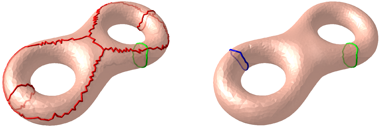
2.3.2. Shortest Loop

According to our main Theorem 2, the shortest non-trivial geodesic loop $\gamma$ must intersect the cut locus $\mathcal{C}$. If we slice the surface along $\mathcal{C}$, then the shortest loop $\gamma$ becomes the shortest path connecting two boundary points. In discrete cases, we use the shortest path on the triangle mesh to approximate the shortest geodesic, and we use the cut graph to approximate the cut locus.

First, we slice the mesh along the cut graph $\mathcal{C}$, to obtain a topological disk $\tilde{M}$, with its boundary denoted as $\partial \tilde{M}$. For each vertex $v\in \mathcal{C}$, we call the number of links in the graph $\mathcal{C}$ adjacent to v as the degree of v. After the pruning in Algorithm 1, all the vertex degrees are greater than or equal to 2. Suppose $v_i\in \mathcal{C}$ with degree $\mathrm{deg}\left(v_i\right)=k$, then the slicing procedure along $\mathcal{C}$ will split $v_i$ to k boundary vertices of $\tilde{M}$, denoted as $\{v_i^1,v_i^2,\dots ,v_i^k\}$. Second, for each $v_i\in \mathcal{C}$ for each pair of $(v_i^j,v_i^k)$, we can compute the shortest path on $\tilde{M}$, using the Dijkstra’s algorithm. Then, we sort the shortest paths according to their total lengths in ascending order. Figure 5 shows the top two shortest loops on the genus-2 surface. The algorithmic pipeline can be found in Algorithm 2.

Algorithm 2 Algorithm for Shortest Loop

Require: A closed triangle mesh M Ensure: The shortest non-trivial loop $\gamma$ of M   1: Compute the cut graph $\mathcal{C}$ of M, using Algorithm 1;   2: Slice M along $\mathcal{C}$, to obtain a simply connected mesh $\tilde{M}$;   3: for all vertex $v_i\in \mathcal{C}$ with $\mathrm{deg}\left(v_i\right)=k$ do   4:     Find all $\{v_i^1,v_i^2,\dots ,v_i^k\}\subset \partial \tilde{M}$;   5:     for all pair $(v_i^j,v_i^k)$ on the boundary $\partial \tilde{M}$ do   6:         Compute the shortest path ${\tilde{\gamma }}_i^{jk}$, using Dijkstra’s algorithm;   7:         Find the loop ${\gamma }_i^{jk}\subset M$ corresponding to ${\tilde{\gamma }}_i^{jk}\subset \tilde{M}$;   8:     end for   9: end for 10: Sort all the shortest loops ${\gamma }_i^{jk}$ in ascending order by their total lengths; 11: Return the shortest loop $\gamma$.

2.3.3. Topological Surgery

Once we have found the shortest loop $\gamma$ on the current mesh M, we can slice M along $\gamma$ to produce a mesh $M_{\gamma }$, where $\gamma$ corresponds to two boundary components of $M_{\gamma }$, namely, ${\gamma }_0$ and ${\gamma }_1$. For the boundary component ${\gamma }_k$, $k=0,1$, we compute the mass center of all its vertices, denoted as $w_k$. For each edge $e\in {\gamma }_k$, we connect e with $w_k$, to form a triangle. All such triangles form a topological disk $D_k$. In this way, we fill the boundary component ${\gamma }_k$ with the topological disk $D_k$. After the hole filling, the genus of the resulting mesh $M_{\gamma }$ is reduced by one. The details are formulated in Algorithm 3.

Algorithm 3 Algorithm for Topological Surgery

Require: A closed triangle mesh M, a non-trivial loop $\gamma$ Ensure: A mesh N with one handle removed from M   1: Slice M along $\gamma$ to obtain a mesh $M_{\gamma }$, $\partial M_{\gamma }={\gamma }_0-{\gamma }_1$;   2: for all boundary component ${\gamma }_k$, $k=0,1$ do   3:     $w_k\leftarrow 0$;   4:     for all vertex $v_i\in {\gamma }_k$ do   5:         $w_k\leftarrow w_k+v_i$;   6:     end for   7:     $w_k\leftarrow w_k/\left|{\gamma }_k\right|$;   8:     for all edge $e_j\in {\gamma }_k$ do   9:         $e_j$ and $w_k$ form a triangle face $f_j^k$; 10:         $M_{\gamma }\leftarrow M_{\gamma }\cup f_j^k$; 11:     end for 12: end for 13: $N\leftarrow M_{\gamma }$.

We combine the above algorithms, to form the topological denoising algorithm in Algorithm 4. First, we compute the Euler number of the mesh $\left(M\right)=\left|V\right|+\left|F\right|-\left|E\right|$, and we find the genus of the surface by $\left(S\right)=2-2g$, where g is the genus of the surface. Second, we find the shortest loop $\gamma$ on the current mesh. Third, we perform topological surgery along $\gamma$, to remove one handle. We repeat this procedure until the genus equals zero.

Algorithm 4 Topological Denoising Algorithm

Require: A high-genus closed triangle mesh M Ensure: The mesh N with all handles removed from M   1: Compute the Euler number $\left(M\right)$ and the genus g of M;   2: Set $M_1\leftarrow M$;   3: for $k=1,2,\dots ,g$ do   4:     Compute the shortest loop ${\gamma }_k$ on $M_k$, using Algorithm 2;   5:     Perform topological surgery on $M_k$ along ${\gamma }_k$, to obtain $M_{k+1}$, using Algorithm 3;   6: end for   7: Set $N\leftarrow M_{g+1}$.

3. Results

All the experiments in this work were carried out on a Ubuntu 20.04 operating system with an AMD Ryzen 7 2700X Eight-Core Processor at 3.7 GHz and 64 GB RAM. The mesh models used in the experiments included general test models for visual illustration and two datasets of colon meshes. The first colon dataset included 10 colon meshes with an average of 100K faces (or triangles). The second colon dataset had a total number of 20 colon meshes with an average of 1000K faces (or triangles). We compared our proposed method to the State-of-the-Art persistent-homology-based method in [24].

3.1. Visual Evaluation on General Test Models

To evaluate the proposed method, we first show the visual evaluation results of the general test models, as they have small numbers of genuses and are easy for visual recognition. Figure 6 shows the general test models, with detected loops highlighted in color. Their topological information is reported in

Table 1. Topological information of general test models, for visual illustration.

Mesh	#Faces	#Genus
Genus-6 model	2 K	6
Double torus	7 K	2
Knotty	10 K	2
Genus-3 model	12 K	3
Amphora	20 K	2
LoveMe	50 K	3
TwoKids	80 K	3
Deco-cube	120 K	5

. The number of faces (or triangles) varies from 2 K to 120 K, and the genuses span from 2 to 6. Given a genus n closed surface, there are n handle loops. As observed from the results in Figure 6, the number of the detected loops in the highlighted color is the same as the numbers of genuses reported in Table 1. Thus, our method can compute all loops correctly.

In the next subsection, we will show the capability of our proposed method for detecting the loops on medical colon datasets and for performing topological denoising for further colon wall flattening in virtual colonoscopy.

3.2. Topological Denoising for Two Colon Datasets

We further evaluated our method on two datasets of colon meshes, which had more complex shapes and high genuses. The colon meshes were reconstructed from CT images in virtual colonoscopy. Figure 7 (left) shows a colon wall mesh with topological noises denoted by green loops. Figure 7 (middle, right) shows the zoom-in views of two regions in the colon wall mesh marked with red boxes. It can be seen that various non-trivial loops in the colon wall surface in different locations can be detected correctly.

The experimental results for the two colon datasets are reported in

Table 2. Comparison, on the first colon dataset with 10 colon meshes, of persistent homology method (denoted by PHM) to our method.

	Success?		All Loops Found?		#Vertices of All Loops
Mesh (#Faces, #Genus)	PHM	Our	PHM	Our	PHM	Our
Colon1 (127 K, 67)	No	Yes	No	Yes	NA	311
Colon2 (44 K, 13)	Yes	Yes	Yes	Yes	65	61
Colon3 (158 K, 31)	No	Yes	No	Yes	NA	141
Colon4 (152 K, 8)	Yes	Yes	Yes	Yes	56	28
Colon5 (140 K, 38)	Yes	Yes	Yes	Yes	660	170
Colon6 (133 K, 30)	Yes	Yes	Yes	Yes	177	141
Colon7 (167 K, 14)	Yes	Yes	Yes	Yes	161	66
Colon8 (176 K, 13)	Yes	Yes	Yes	Yes	131	67
Colon9 (236 K, 7)	Yes	Yes	Yes	Yes	24	23
Colon10 (147 K, 19)	Yes	Yes	Yes	Yes	118	74

and

Table 3. Comparison, on the second colon dataset with 20 colon meshes, of persistent homology method (denoted by PHM) to our method.

	Success?		All Loops Found?		#Vertices of All Loops
Mesh (#Faces, #Genus)	PHM	Our	PHM	Our	PHM	Our
Colon1 (1091 K, 4)	Yes	Yes	Yes	Yes	77	24
Colon2 (1679 K, 6)	Yes	Yes	Yes	Yes	115	65
Colon3 (1679 K, 6)	Yes	Yes	Yes	Yes	118	65
Colon4 (1528 K, 26)	Yes	Yes	Yes	Yes	1104	492
Colon5 (1181 K, 17)	Yes	Yes	Yes	Yes	231	119
Colon6 (1350 K, 12)	Yes	Yes	Yes	Yes	321	124
Colon7 (1185 K, 3)	Yes	Yes	Yes	Yes	60	36
Colon8 (1144 K, 9)	Yes	Yes	Yes	Yes	158	107
Colon9 (1389 K, 17)	Yes	Yes	Yes	Yes	675	436
Colon10 (1259 K, 2)	Yes	Yes	Yes	Yes	11	11
Colon11 (1204 K, 4)	Yes	Yes	Yes	Yes	116	58
Colon12 (1692 K, 2)	Yes	Yes	Yes	Yes	122	36
Colon13 (1236 K, 11)	Yes	Yes	Yes	Yes	206	129
Colon14 (1300 K, 11)	Yes	Yes	Yes	Yes	298	250
Colon15 (1428 K, 17)	Yes	Yes	Yes	Yes	326	213
Colon16 (1631 K, 22)	No	Yes	No	Yes	NA	410
Colon17 (1531 K, 8)	Yes	Yes	Yes	Yes	409	277
Colon18 (1774 K, 11)	Yes	Yes	Yes	Yes	210	83
Colon19 (1482 K, 18)	Yes	Yes	Yes	Yes	483	454
Colon20 (1202 K, 19)	No	Yes	No	Yes	NA	177

, respectively. For the first colon dataset, as shown in Table 2, our method was successfully run on all 10 colon data, and it detected all the loops in the noisy colon data. By comparison, the persistent homology method could only be executed on 8 colon data, and it failed on 2 colon data. This demonstrates that our method is more robust than the persistent homology method. Moreover, the lengths (number of vertices) of detected loops in all 10 colon data were much shorter by our method than by the persistent homology method, indicating the advantage of our method for computing and obtaining shorter detected loops.

According to the experimental results shown in Table 3 for the second colon dataset, our method outperforms the persistent homology method, in terms of robustness and computation of shorter loops. It can be seen that among the 20 colon data, our method successfully computed the loops on all 20 colon data, whereas the persistent homology method failed on 2 colon data. Also, our method was able to detect all loops with shorter lengths than those of the persistent homology method. Therefore, the experimental results on both colon datasets demonstrate the effectiveness and robustness of our method.

3.3. Colon Flattening in Virtual Colonoscopy

To evaluate the full efficacy of the proposed method, we applied the method to the flattening of a 3D colon wall surface to a 2D plane in virtual colonoscopy. The top row in Figure 8 shows the original 3D colon surface without denoising and the corresponding colon surface after denoising, respectively. The 3D colon wall surface after topological denoising, using our method, was then flattened to the 2D plane via surface parameterization, which is shown in the bottom row in Figure 8. A 2D visualization of the flattened colon wall surface provides physicians with a good alternative for the detection of colorectal polyps, in comparison to a traditional 3D endoscopic view. Also, the supplementary geometric and texture features in the 2D flattened colon wall can be used in practice, to improve polyp detection rates.

We also applied our method to colon data containing a clinically detected polyp of size ≥ 10 mm. Figure 9a shows the result of the colon surface by our topological denoising method, where the blue curve indicates the curve along which the 3D colon surface is cut, for colon wall flattening to a 2D plane. Figure 9b gives a different view of a 3D colon surface, and the yellow arrow indicates the location of the polyp, which is highlighted by the red points. Endoscopic views of the polyp on the colon wall are shown in Figure 9c,d, where the red points are used to represent the polyp area. After the 3D colon wall surface was flattened to a 2D plane, we obtained a 2D visualization of the polyp on the flattened colon surface, as seen in Figure 9e. This alternative view of the polyp was conducive to detecting and locating the polyp.

4. Conclusions

In this work, we have proposed a novel topological denoising method based on homotopy theory. We applied the method to colon surface denoising in virtual colonoscopy. The method is, in essence, computed in an iterative fashion. In terms of computational steps, the algorithm mainly includes computations of cut graph and shortest loops, as well as performing topological surgery. The method is not only mathematically rigorous but also computationally robust. We evaluated the proposed method on two datasets of colon meshes, and we conducted comparative experiments, to validate the method. In comparison to the State-of-the-Art topological denoising method, our method outperforms the existing method, in terms of robustness and effectiveness.

From the perspective of applications, the proposed method has the potential to be applied in topological denoising tasks for other organs of interest in the medical imaging field. In future work, we will explore in this direction, and we will apply the proposed method to more medical imaging tasks.

References

- Yao, J.; Li, J.; Summers, R. CT colonography computer-aided polyp detection using topographical height map. In Proceedings of the 2007 IEEE International Conference on Image Processing, San Antonio, TX, USA, 16–19 September 2007; Volume 5, pp. V-21–V-24. [Google Scholar]
- Lee, J.G.; Kim, J.H.; Kim, S.H.; Park, H.S.; Choi, B.I. A straightforward approach to computer-aided polyp detection using a polyp-specific volumetric feature in CT colonography. Comput. Biol. Med. 2011, 41, 790–801. [Google Scholar] [CrossRef]
- Umehara, K.; Näppi, J.J.; Hironaka, T.; Regge, D.; Ishida, T.; Yoshida, H. Deep ensemble learning of virtual endoluminal views for polyp detection in CT colonography. In Proceedings of the Medical Imaging 2017: Computer-Aided Diagnosis, SPIE, Orlando, FL, USA, 13–16 February 2017; Volume 10134, pp. 108–113. [Google Scholar]
- Ren, Y.; Ma, J.; Xiong, J.; Chen, Y.; Lu, L.; Zhao, J. Improved false positive reduction by novel morphological features for computer-aided polyp detection in CT colonography. IEEE J. Biomed. Health Inform. 2018, 23, 324–333. [Google Scholar] [CrossRef]
- Pomeroy, M.; Wang, Y.; Banerjee, A.; Abbasi, A.; Barish, M.; Sun, E.; Bucobo, J.C.; Pickhardt, P.J.; Liang, Z. Integration of optical and virtual colonoscopy images for enhanced classification of colorectal polyps. In Proceedings of the Medical Imaging 2020: Computer-Aided Diagnosis, SPIE, Houston, TX, USA, 16–19 February 2020; Volume 11314, pp. 139–144. [Google Scholar]
- Mirhosseini, S.; Gutenko, I.; Ojal, S.; Marino, J.; Kaufman, A. Immersive virtual colonoscopy. IEEE Trans. Vis. Comput. Graph. 2019, 25, 2011–2021. [Google Scholar] [CrossRef]
- Mathew, S.; Nadeem, S.; Kumari, S.; Kaufman, A. Augmenting colonoscopy using extended and directional cyclegan for lossy image translation. In Proceedings of the IEEE/CVF Conference on Computer Vision and Pattern Recognition, Seattle, WA, USA, 13–19 June 2020; pp. 4696–4705. [Google Scholar]
- Kotecha, S.; Vasudevan, A.; Holla, V.K.; Kumar, S.; Pruthviraja, D.; Latte, M.V. 3D visualization cloud based model to detect and classify the polyps according to their sizes for CT colonography. J. King Saud Univ.-Comput. Inf. Sci. 2022, 34, 4943–4955. [Google Scholar] [CrossRef]
- Nappi, J.J.; Hironaka, T.; Wu, D.; Yoshida, S.R.; Gupta, R.; Tachibana, R.; Taguchi, K.; Yoshida, H. Automated detection of colorectal polyps in photon-counting CT colonography. In Proceedings of the Medical Imaging 2023: Imaging Informatics for Healthcare, Research, and Applications, SPIE, San Diego, CA, USA, 19–24 February 2023; Volume 12469, pp. 187–191. [Google Scholar]
- Chen, S.; Li, Y.F.; Zhang, J. Vision processing for realtime 3-D data acquisition based on coded structured light. IEEE Trans. Image Process. 2008, 17, 167–176. [Google Scholar] [CrossRef]
- Bi, Z.; Wang, L. Advances in 3D data acquisition and processing for industrial applications. Robot. Comput. Integr. Manuf. 2010, 26, 403–413. [Google Scholar] [CrossRef]
- Henderson, P.; Tsiminaki, V.; Lampert, C.H. Leveraging 2d data to learn textured 3d mesh generation. In Proceedings of the IEEE/CVF Conference on Computer Vision and Pattern Recognition, Seattle, WA, USA, 13–19 June 2020; pp. 7498–7507. [Google Scholar]
- Glaßer, S.; Berg, P.; Neugebauer, M.; Preim, B. Reconstruction of 3D surface meshes for blood flow simulations of intracranial aneurysms. In Proceedings of the Conference of the German Society for Computer and Robotic Assisted Surgery, London, UK, 10–11 September 2015; pp. 163–168. [Google Scholar]
- Kong, F.; Wilson, N.; Shadden, S. A deep-learning approach for direct whole-heart mesh reconstruction. Med. Image Anal. 2021, 74, 102222. [Google Scholar] [CrossRef]
- Lee, S.; Chen, L.; Wang, J.; Liniger, A.; Kumar, S.; Yu, F. Uncertainty guided policy for active robotic 3d reconstruction using neural radiance fields. IEEE Robot. Autom. Lett. 2022, 7, 12070–12077. [Google Scholar] [CrossRef]
- Di Angelo, L.; Di Stefano, P.; Guardiani, E. A review of computer-based methods for classification and reconstruction of 3D high-density scanned archaeological pottery. J. Cult. Herit. 2022, 56, 10–24. [Google Scholar] [CrossRef]
- Maboudi, M.; Homaei, M.; Song, S.; Malihi, S.; Saadatseresht, M.; Gerke, M. A Review on Viewpoints and Path Planning for UAV-Based 3D Reconstruction. IEEE J. Sel. Top. Appl. Earth Obs. Remote. Sens. 2023, 16, 5026–5048. [Google Scholar] [CrossRef]
- Erickson, J.; Whittlesey, K. Greedy optimal homotopy and homology generators. In Proceedings of the SODA, Vancouver, BC, Canada, 23–25 January 2005; Volume 5, pp. 1038–1046. [Google Scholar]
- Chen, C.; Freedman, D. Quantifying homology classes. arXiv 2008, arXiv:0802.2865. [Google Scholar]
- Dey, T.K.; Li, K.; Sun, J.; Cohen-Steiner, D. Computing geometry-aware handle and tunnel loops in 3d models. In ACM SIGGRAPH 2008 Papers; Association for Computing Machinery: New York, NY, USA, 2008; pp. 1–9. [Google Scholar]
- Zhou, Q.Y.; Ju, T.; Hu, S.M. Topology repair of solid models using skeletons. IEEE Trans. Vis. Comput. Graph. 2007, 13, 675–685. [Google Scholar] [CrossRef]
- Dey, T.K.; Li, K.; Sun, J. On computing handle and tunnel loops. In Proceedings of the 2007 International Conference on Cyberworlds (CW’07), Hannover, Germany, 24–26 October 2007; pp. 357–366. [Google Scholar]
- Dey, T.K.; Li, K.; Sun, J. Computing handle and tunnel loops with knot linking. Comput.-Aided Des. 2009, 41, 730–738. [Google Scholar] [CrossRef]
- Dey, T.K.; Fan, F.; Wang, Y. An efficient computation of handle and tunnel loops via Reeb graphs. ACM Trans. Graph. (TOG) 2013, 32, 1–10. [Google Scholar] [CrossRef]
- Weinrauch, A.; Seidel, H.P.; Mlakar, D.; Steinberger, M.; Zayer, R. A Variational Loop Shrinking Analogy for Handle and Tunnel Detection and Reeb Graph Construction on Surfaces. arXiv 2021, arXiv:2105.13168. [Google Scholar] [CrossRef]
- Gao, M.; Chen, C.; Zhang, S.; Qian, Z.; Metaxas, D.; Axel, L. Segmenting the papillary muscles and the trabeculae from high resolution cardiac CT through restoration of topological handles. In Proceedings of the 23rd International Conference on Information Processing in Medical Imaging, Asilomar, CA, USA, 28 June–3 July 2013; pp. 184–195. [Google Scholar]
- Wu, P.; Chen, C.; Wang, Y.; Zhang, S.; Yuan, C.; Qian, Z.; Metaxas, D.; Axel, L. Optimal topological cycles and their application in cardiac trabeculae restoration. In Proceedings of the 25th International Conference on Information Processing in Medical Imaging, Boone, NC, USA, 25–30 June 2017; pp. 80–92. [Google Scholar]
- Brezovsky, J.; Chovancova, E.; Gora, A.; Pavelka, A.; Biedermannova, L.; Damborsky, J. Software tools for identification, visualization and analysis of protein tunnels and channels. Biotechnol. Adv. 2013, 31, 38–49. [Google Scholar] [CrossRef]
- Paik, D.S.; Beaulieu, C.F.; Jeffrey Jr, R.B.; Karadi, C.A.; Napel, S. Visualization modes for CT colonography using cylindrical and planar map projections. J. Comput. Assist. Tomogr. 2000, 24, 179–188. [Google Scholar] [CrossRef]
- Vilanova Bartroli, A.; Wegenkittl, R.; König, A.; Gröller, E.; Sorantin, E. Virtual colon flattening. In Proceedings of the Data Visualization 2001: Proceedings of the Joint Eurographics—IEEE TCVG Symposium on Visualization in Ascona, Ascona, Switzerland, 28–30 May 2001; pp. 127–136. [Google Scholar]
- Balogh, E.; Sorantin, E.; Nyul, L.; Palagyi, K.; Kuba, A.; Werkgartner, G.; Spuller, E. Colon unraveling based on electronic field: Recent progress and future work. Proc. SPIE 2002, 4681, 713–721. [Google Scholar]
- Hong, W.; Gu, X.; Qiu, F.; Jin, M.; Kaufman, A. Conformal virtual colon flattening. In Proceedings of the 2006 ACM Symposium on Solid and Physical Modeling, Wales, UK, 6–8 June 2006; pp. 85–93. [Google Scholar]
- Hong, W.; Qiu, F. A pipeline for computer aided polyp detection. IEEE Trans. Vis. Comput. Graph. 2006, 12, 861–868. [Google Scholar] [CrossRef]
- Wang, Z.; Li, B.; Liang, Z. Feature-based texture display for detection of polyps on flattened colon volume. In Proceedings of the 2005 IEEE Engineering in Medicine and Biology 27th Annual Conference, Shanghai, China, 17–18 January 2006; pp. 3359–3362. [Google Scholar]
- Gurijala, K.C.; Shi, R.; Zeng, W.; Gu, X.; Kaufman, A. Colon flattening using heat diffusion riemannian metric. IEEE Trans. Vis. Comput. Graph. 2013, 19, 2848–2857. [Google Scholar] [CrossRef]
- Wang, H.; Chen, Y.; Li, L.; Pan, H.; Gu, X.; Liang, Z. A novel colon wall flattening model for computed tomographic colonography: Method and validation. Comput. Methods Biomech. Biomed. Eng. Imaging Vis. 2015, 3, 213–221. [Google Scholar] [CrossRef]
- Kreiser, J.; Meuschke, M.; Mistelbauer, G.; Preim, B.; Ropinski, T. A survey of flattening-based medical visualization techniques. Comput. Graph. Forum 2018, 37, 597–624. [Google Scholar] [CrossRef]
- Eulzer, P.; Richter, K.; Meuschke, M.; Hundertmark, A.; Lawonn, K. Automatic Cutting and Flattening of Carotid Artery Geometries. In Proceedings of the VCBM, Paris, France, 22–24 September 2021; pp. 79–89. [Google Scholar]
- Zeng, W.; Shi, R.; Su, Z.; Gu, D.X. Efficient Topological Cleaning for Visual Colon Surface Flattening. In Abdomen Thoracic Imaging; Springer: Berlin/Heidelberg, Germany, 2014; pp. 421–441. [Google Scholar]
- Armstrong, M.A. Basic Topology; Springer Science & Business Media: Berlin/Heidelberg, Germany, 2013. [Google Scholar]