Quasi-Semilattices on Networks

Abstract

This paper introduces a representation of subnetworks of a network $\Gamma$ consisting of a set of vertices and a set of relations, where relations are the primitive structures of a network. It is proven that all connected subnetworks of a network $\Gamma$ form a quasi-semilattice $\mathcal{L}(\Gamma )$, namely a network quasi-semilattice.Two equivalences $\sigma$ and $\delta$ are defined on $\mathcal{L}(\Gamma )$. Each $\delta$ class forms a semilattice and also has an order structure with the maximum element and minimum elements. Here, the minimum elements correspond to spanning trees in graph theory. Finally, we show how graph inverse semigroups, Leavitt path algebras and Cuntz–Krieger graph $C^{*}$-algebras are constructed in terms of relations.

1. Introduction

A network $\Gamma =(V_{\Gamma },T_{\Gamma })$ consists of sets $V_{\Gamma }$ and $T_{\Gamma }$. The elements of $V_{\Gamma }$ are called vertices, and the elements of $T_{\Gamma }$ are called relations or edges. Here, we prefer to call the elements of $T_{\Gamma }$ relations. A relation is called a correlation if it connects two vertices and is drawn as an undirected arrow. A network is called a correlation network if each relation is a correlation. A correlation network is simple if it does not contain any self-loops or parallel relations. In graph theory, a simple correlation network is called a simple undirected graph. In order to identify detailed logic relationships between proteins on the basis of genomic data, Bowers et al. introduced a new concept, higher-order logic relations, and further higher-order logic networks were built [1]. Compared with higher-order logic relations, in this paper, a relation is a first-order logic relation if it connects two vertices and is drawn as a directed arrow starting at one vertex and pointing to another vertex. A network is called a first-order logic network if each relation is a first-order logic relation. Actually, a first-order logic network is called a directed graph in graph theory. Here, we prefer to call it a first-order logic network. A relation is a higher-order logic relation if it connects more than two vertices and is drawn as a directed arrow starting at A and pointing to B, where A and B are nonempty sets of vertices with $A\cap B=\varnothing$. A relation is a logic relation if it is either a first-order logic relation or a higher-order logic relation. A network is called a logic network if each relation is a logic relation. A network is said to be a higher-order logic network if it is a logic network and contains at least one higher-order logic relation. A network $\Delta =(V_{\Delta },T_{\Delta })$ is a subnetwork of $\Gamma =(V_{\Gamma },T_{\Gamma })$ if $V_{\Delta }\subseteq V_{\Gamma }$ and $T_{\Delta }\subseteq T_{\Gamma }$.

Networks are abstract models of real complex systems, and thus networks have some properties of real complex systems, such as modular structures or communities [2,3] of networks reflecting the small-word property; that is, things with similar attributes are often prone to clustering together. The detection of communities in a network is of great significance for understanding network structures and dynamics. The attributes of communities have been successfully applied in various fields. In protein interaction networks, proteins with similar functions often exist in the form of communities [4]. Therefore, the function of unknown proteins can be predicted based on the functions of known proteins within the same community. In the WWW network, by analyzing communities, people can obtain pages with relevant or similar themes without knowing the text content of the webpage [5].

A community is an important and ubiquitous structural characteristic in complex networks. Up to now, many theories and methods have been proposed for in-depth research and analysis of communities. These algorithms are mainly divided into the following categories: splitting methods [6,7], merging methods [8], modularity-based optimization and extension methods [9], random walk model algorithms [10,11], multi-objective optimization methods [12] and spectral clustering [13], among others. Such algorithms were proposed based on a view that in a network, vertices are regarded as research subjects (primitives), and the relations between vertices are regarded as the correlation attribute of vertices. In addition, these algorithms are suitable for detecting communities in simple correlation networks or first-order logic networks. In particular, spectral clustering methods depend on the Laplacian matrix of a network. While a higher-order logic network [1] is difficult to represent with a matrix, this puts forward a new topic on the algebraic representation of networks. Using a “tensor symbol” to represent a relation of a network is introduced first in this paper, which can be regarded as a generalization of adjacency matrices. It is suitable for correlation (or logic) networks. In this paper, correlation networks, first-order logic networks and higher-order logic networks extended by the research in [1] are collectively referred to as general networks, which are the main research object of this paper.

Another perspective for studying networks is to take relations as the research objects, such as paths in first-order logic networks. Here, a path in a first-order logic network $\Gamma =(V_{\Gamma },T_{\Gamma })$ is a finite sequence $p=t_1{t}_2\cdots t_n$ of relations $t_i\in T_{\Gamma }$ with $\mathbf{r}\left(t_i\right)=\mathbf{s}\left(t_{i+1}\right)$ for $i=1,\dots ,n-1$, where $\mathbf{r}\left(t_i\right)$ is the target of $t_i$ and $\mathbf{s}\left(t_i\right)$ is the source of $t_i$. Ash and Hall [14] first introduced graph inverse semigroups by using the paths of first-order logic networks. Furthermore, it was proven that two first-order logic networks are isomorphic if and only if their corresponding graph inverse semigroups are isomorphic [15]. This shows a way to use algebraic methods to study networks. Notice that paths and communities are both special subnetworks of a network. It is meaningful to use algebraic methods to investigate the subnetworks of a network. To accomplish this, we take relations as the research objects, give a representation of subnetworks (or networks) and further build an algebraic system $\mathcal{L}(\Gamma )$ consisting of certain subnetworks of a network $\Gamma$, called network quasi-semilattices. In addition, with respect to the partial order defined in Section 6, it was found that the minimum elements in a congruence class, say $l\delta$ of $\mathcal{L}(\Gamma )$, are spanning trees generated by all relations of $l\delta$. As we all know, in network routing algorithms, a more universal solution to resolve deadlocks is to organize an acyclic subnetwork. The simplest way to use an acyclic subnetwork is to use a zero-rooted spanning tree [16]. Thus, it is helpful to detect spanning trees by investigating the minimum elements in the $\delta$ classes with respect to the partial order defined in Section 6.

The structure of this paper is as follows. Section 2 gives some basic concepts such as quasi-semilattices. Section 3 introduces the definitions of networks and presents the notation used in the context. In Section 4, two binary operations, called chain addition of relations and reducing of 2-chains, are introduced. The set of all 2-chains of a network $\Gamma$ with respect to reducing generates a quasi-semilattice $\mathcal{L}(\Gamma )$ in which every element is idempotent and the binary operation is commutative but non-associative. In Section 5, two equivalent relations $\sigma$ and $\delta$ are given on $\mathcal{L}(\Gamma )$. We show that $\delta$ is a congruence, and each $\delta$-class is a semilattice which is an idempotent commutative semigroup. Furthermore, the relationship between two $\delta$ classes is discussed, and we give a condition where two $\delta$ classes are isomorphic. In Section 6, a partial order relation ⪯ is given, and the local maximum and the minimum elements of the $\delta$ classes are investigated with respect to ⪯. We show that the minimum elements of a $\delta$ class, say $l\delta$, are spanning trees generated by all relations of $l\delta$. In Section 7, we claim that graph inverse semigroups [14], Leavitt path algebras [17] and Cuntz–Krieger graph $C^{*}$-algebras [18,19] can be generated by chain addition of a first-order logic network. Here, graph inverse semigroups, Leavitt path algebras and Cuntz–Krieger graph $C^{*}$-algebras consist of only thr paths of a first-order logic network, which are special subnetworks of a network, while the elements in $\mathcal{L}(\Gamma )$ are not only the paths but also other subnetworks, such as branchings.

This paper introduces a representation of subnetworks of a general network, which is different from the traditional network research method taking vertices as the research object. The research on the quasi-semilattice generated by relations is applicable to correlation networks and logic networks. Relations generate not only the path of a general network but also all connected subnetworks of the network (such as branches, especially in higher-order logic networks.) The traditional path cannot represent all of the higher-order subnetworks. Therefore, the representation of (sub)networks not only introduces new algebraic theory but also provides a new method for the study of networks.

2. Preliminaries

In this section, we recall some basic notions used in the following sections. More details can be found in [20].

Definition 1.

A nonempty set S together with a binary operation ∗ is called a quasi-semilattice if for any $a,b\in S$, $a\ast a=a$, $a\ast b=b\ast a\in S$, and there exist $a,b,c\in S$ such that $(a\ast b)\ast c\ne a\ast (b\ast c)$.

It is necessary to remark that a semilattice $(S,\ast )$ is a commutative idempotent semigroup; that is, $a\ast a=a$, $a\ast b=b\ast a\in S$ and $(a\ast b)\ast c=a\ast (b\ast c)$ for any $a,b,c\in S$. Clearly, whether the associative law is satisfied or not is the fundamental difference between semilattices and quasi-semilattices. A magma is a nonempty set M together with a binary operation ∗ such that $a\ast b\in M$ for any $a,b\in M$. The quasi-semilattice defined here is a commutative idempotent magma which is non-associative. An example of quasi-semilattices with three elements follows. Let $S=\{a,b,c\}$ have the following Cayley table with respect to ∗ (see

Table 1. Cayley table of S.

∗	a	b	c
a	a	c	b
b	c	b	a
c	b	a	c

).

Clearly, S is closed and commutative with respect to ∗, and for each $x\in S$, we have $x\ast x=x$. Notice that $(a\ast b)\ast c=c\ne a=a\ast (b\ast c)$. Hence, $(S,\ast )$ forms a quasi-semilattice.

Definition 2.

Let $(Y,\ast )$ be a quasi-semilattice. A nonempty subset H of Y is called a sub-semilattice of Y if $(H,\ast )$ forms a semilattice.

Definition 3.

Let $(Y,·)$ and $(Y^{\prime },\circ )$ be two quasi-semilattice, and let ξ be a map from Y to $Y^{\prime }$. The map ξ is a homomorphism if for any $a,b\in Y$, $\xi (a·b)=\xi \left(a\right)\circ \xi \left(b\right)$. A homomorphism ξ is an epimorphism if ξ is surjective.

An equivalence $\rho$ on an algebraic system $(A,\ast )$ is a congruence with respect to ∗ if $\rho$ is left and right compatible with respect to ∗; that is, for any $a,b,c\in A$, if $(a,b)\in \rho$, then $(c\ast a,c\ast b)\in \rho$ and $(a\ast c,b\ast c)\in \rho$. If the operation is commutative, then a left compatible relation is also right compatible.

3. General Networks

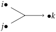
A network $\Gamma =(V_{\Gamma },T_{\Gamma })$ consists of a set $V_{\Gamma }$ of vertices and a set $T_{\Gamma }$ of edges (termed relations in this context). A relation in $T_{\Gamma }$ is said to be a correlation if it connects two vertices, and it is drawn as an undirected arrow. If a correlation $t\in T_{\Gamma }$ connects two vertices u and v, then we write t as $T_A$; that is, $t=T_A$, where $A=\{u,v\}$ and we call A the covariant index of t. We define $\mathbf{s}\left(T_A\right)=A$. A relation in $T_{\Gamma }$ is said to be a logic if it is an ordered pair of disjoint subsets of $V_{\Gamma }$. The first component of a logic relation t is called the covariant index (or source) of t, denoted by $\mathbf{s}\left(t\right)$, and the second component of t is called the contra-variant index (or range) of t, denoted by $\mathbf{r}\left(t\right)$. To emphasize $\mathbf{s}\left(t\right)$ and $\mathbf{r}\left(t\right)$, we write t as $T_A^B$, where $\mathbf{s}\left(t\right)=A$ and $\mathbf{r}\left(t\right)=B$. A logic relation $t\in T_{\Gamma }$ is called an m-n order logic relation if $\left|\mathbf{s}\right(t\left)\right|=m$ and $\left|\mathbf{r}\right(t\left)\right|=n$, $m,n\in \mathbb{N}$. In particular, an m-n-order logic relation is called an mth order logic relation if $n=1$. For example, a first-order logic relation is a relation whose covariant index and contra-variant index are two disjoint singleton subsets of $V_{\Gamma }$, such as with one vertex i affecting another one j, drawn as $i•\to •j$, and a second-order logic relation refers to a logic relation where two vertices jointly affect one vertex; that is, we have the following:

.

A network $\Gamma =(V_{\Gamma },T_{\Gamma })$ is a correlation (or logic) network if each relation in $T_{\Gamma }$ is a correlation (or logic relation). A simple correlation network is a correlation network which does not contain any self-loops or parallel relations. A first-order logic network is a logic network in which each relation is a first-order logic relation. Actually, in graph theory a simple correlation network is called a simple undirected graph, and a first-order logic network is a directed graph. In this context, we prefer first-order logic networks rather than directed graphs. A higher-order logic network is a logic network which contains at least one higher-order logic relation. In this paper, correlation networks and logic networks are collectively referred to as “general networks”.

A network $\Delta =(V_{\Delta },T_{\Delta })$ is said to be a subnetwork of $\Gamma =(V_{\Gamma },T_{\Gamma })$ if $V_{\Delta }\subseteq V_{\Gamma }$ and $T_{\Delta }\subseteq T_{\Gamma }$. A directed path in a first-order logic network $\Gamma =(V_{\Gamma },T_{\Gamma })$ is a finite sequence $p=e_1{e}_2\dots e_k$ of the relations $e_i\in T_{\Gamma }$ with $\mathbf{r}\left(e_i\right)$$=\mathbf{s}\left(e_{i+1}\right)$ for $i=1,\dots ,k-1$. We define $\mathbf{s}\left(p\right)=\mathbf{s}\left(e_1\right)$ and $\mathbf{r}\left(p\right)=\mathbf{r}\left(e_k\right)$.

Let $\Gamma =(V_{\Gamma },T_{\Gamma })$ be a general network and $T_A^B\in T_{\Gamma }$. If $B=\varnothing$, then $T_A^B=T_A$ is a correlation. We define the index of a relation $T_A^B$ (B can possibly be the empty set) to be $A\cup B$, denoted by $I\left(T_A^B\right)=A\cup B$. We claim that all networks under consideration in this paper will be correlation networks, first-order logic networks or higher-order logic networks. Also, we only consider finite networks; that is, $\left|V_{\Gamma }\right|<\infty$ and $\left|T_{\Gamma }\right|<\infty$. Let $\Gamma =(V_{\Gamma },T_{\Gamma })$ be a network. Suppose that $\left|T\right|=n$, $n\in \mathbb{N}$. By sorting the elements in $T_{\Gamma }$, we write $T_{\Gamma }$ as $\{t_1,t_2,\dots ,t_n\}$; that is, $T_{\Gamma }=\{t_1,t_2,\dots ,t_n\}$.

4. Quasi-Semilattices

The aim of this section is to generate a quasi-semilattice using the relations of a network.

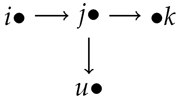
It is easy to see that two different relations are connected through common vertices in a network. For example, in a first-order logic network $\Gamma$ (see Figure 1), we set $t_1=T_i^j$ (i.e., $i•\to j•$) and $t_2=T_j^k$ (i.e., $j•\to u•$). Then, $t_1$ and $t_2$ have a common vertex j, and so we combine the same vertex j to obtain a subnetwork $i•\to j•\to •k$. Naturally, it is a binary operation on relations. We call it the chain addition of relations, written as ⊕. Therefore, $t_1\oplus t_2=\oplus (t_1,t_2)$, where $\oplus (t_1,t_2)$ denotes the subnetwork $i•\to j•\to •k$ obtained by combining the same vertex.

Definition 4.

Let $\Gamma =(V_{\Gamma },T_{\Gamma })$. For any $t,t_1,t_2\in T_{\Gamma }$, we have

$$t_1\oplus t_2=\left\{\begin{array}{cc}\oplus (t_1,t_2)\hfill & \mathrm{if}{t}_1\ne t_2\mathrm{and}I\left(t_1\right)\cap I\left(t_2\right)\ne \varnothing \hfill \\ t_1\left(or{t}_2\right)\hfill & \mathrm{if}{t}_1=t_2\hfill \\ \varnothing \hfill & \mathrm{otherwise},\hfill \end{array}\right.$$

$$t\oplus \varnothing =\varnothing \oplus t=\varnothing ,$$

where $(t_1,t_2)$ denotes the set $\{t_1,t_2\}$ in $\oplus (t_1,t_2)$, $\oplus (t_1,t_2)$ denotes the subnetwork obtained by combining all the same indexes of $t_1$ and $t_2$ and ∅ denotes the empty relation.

Here, we should stress that in Definition 4, $\oplus (t_1,t_2)=\oplus (t_2,t_1)$, as $(t_1,t_2)$ denotes the set whose elements are $t_1$ and $t_2$. We call $\oplus (t_1,t_2)$ a 2-chain.

In a simple correlation network, there exists only one type of 2-chain; that is, we have

$$“j_1•—•i_1—•j_2^{″}$$

for $T_A$ and $T_B$, where $A=\{i_1,j_1\}$ and $B=\{i_1,j_2\}$. In a higher-order logic network only consisting of first-order and second-order logic relations and in which no two relations have the same covariant index and contra-variant index, there exist three combinations to form 2-chains: Case I (two first-order logic relations), Case II (one first-order logic relation and one second-order logic relation) and Case III (two second-order logic relations). For Case I, according to the combination of the same index among the contra-variant index and covariant index of two different first-order logic relations $T_{i_1}^{k_1}$ and $T_{i_2}^{k_2}$, there are three types of 2-chains:

(1) $i_1•⟶•k_1⟶•k_2$ if $k_1=i_2$;

(2) $k_1•⟵•i_1⟶•k_2$ if $i_1=i_2$;

(3) $i_1•⟶•k_1⟵•i_2$ if $k_1=k_2$,

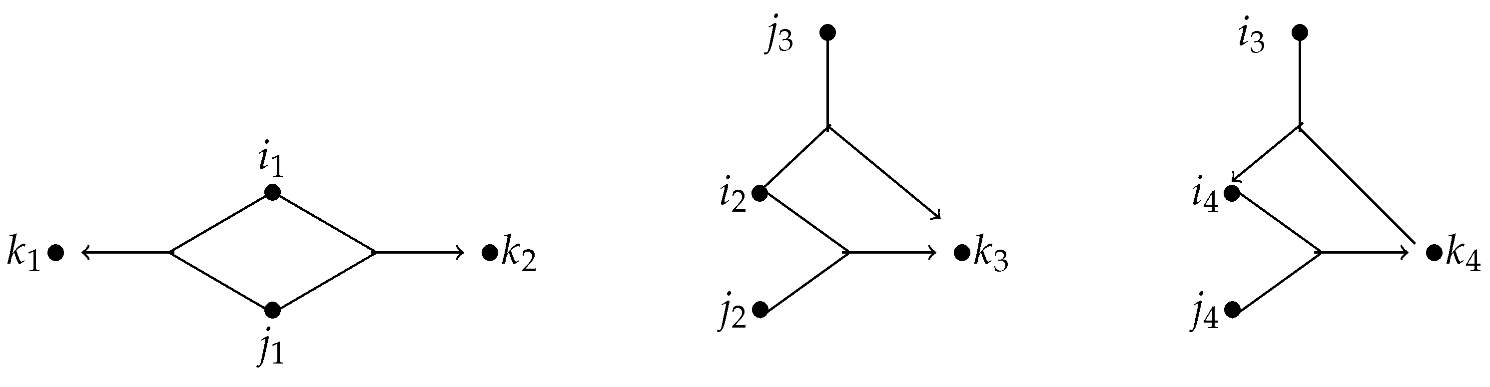
where $i_1,i_2,k_1,k_2\in V_{\Gamma }$. For Case II and Case III, there are five and seven types, respectively. Figure 2 is an example which shows three out of seven types in Case III.

Definition 5.

A network $\Gamma =(V_{\Gamma },T_{\Gamma })$ is said to be connected if for any two different relations $t_i,t_j\in T_{\Gamma }$, there exist $t_{k_1},t_{k_2},\dots ,t_{k_m}\in T_{\Gamma }$ such that

$$t_i=t_{k_1},\oplus (t_{k_{𝓁}},t_{k_{𝓁+1}})\ne \varnothing ,t_{k_m}=t_j,$$

where $𝓁=1,2,\dots ,m-1$.

Next, we will use 2-chains to generate a subnetwork. To accomplish this, we first give an example. Let $\Gamma =\left(V_{\Gamma }{T}_{\Gamma }\right)$ be a general network, and let $t_1,t_2,t_3\in T_{\Gamma }$ be such that $t_i\ne t_j$ and $I\left(t_i\right)\cap I\left(t_j\right)\ne \varnothing$ for $i\ne j$, $i,j\in \{1,2,3\}$. Let $\Delta$ be a subnetwork consisting of $t_1,t_2$ and $t_3$, obtained through $t_1\oplus t_2$ and $t_1\oplus t_3$. It is obvious that $\Delta$ can be obtained by reducing the common relation $t_1$ in the two 2-chains $\oplus (t_1,t_2)$ and $\oplus (t_1,t_3)$ to one. Therefore, we write $\Delta =\oplus (t_1,t_2,t_3|\oplus (t_1,t_2),\oplus (t_1,t_3))$.

To give a formal definition of reducing two 2-chains, we introduce some notation. For any $t_i\in T$, we write $t_i=\oplus (t_i,t_i)$, simply denoted by $l_{ii}$. For any two different relations $t_i,t_j\in T$, if $t_i\oplus t_j=\oplus (t_i,t_j)\ne \varnothing$, then $\oplus (t_i,t_j)$ is simply written as $l_{ij}$, where the subscripts i and j of $l_{ij}$ are unordered; that is, $l_{ij}=l_{ji}$. We set $N=\{1,2,\dots ,n\}$ and let $T_{n2}$ denote the set of all nonempty 2-chains generated by all relations in T; that is, $T_{n2}=\left\{l_{ij}\right|i,j=1,2,\dots ,n;l_{ij}\ne \varnothing \}$. The reducing operation is defined in the following:

Definition 6.

A binary operation $\mathring{\cup }$ on $T_{n2}$, called reducing, is defined by the rule that for any $l_{ii}$, $l_{jj}$, $l_{i_1{j}_1}$ and $l_{i_2{j}_2}$ in $T_{2n}$, the following is true:

$$l_{i_1{j}_1}\mathring{\cup }{l}_{i_2{j}_2}=\left\{\begin{array}{cc}\oplus (t_1,t_2,t_3|l_{i_1{j}_1},l_{i_2{j}_2})\hfill & \mathrm{if}{l}_{i_1{j}_1}\ne l_{i_2{j}_2}\hfill \\ \hfill & \mathrm{and}(t_{i_1},t_{j_1})\cap (t_{i_2},t_{j_2})\ne \varnothing \hfill \\ l_{i_1{j}_1}\left(\mathrm{or}{l}_{i_2{j}_2}\right)\hfill & \mathrm{if}{l}_{i_1{j}_1}=l_{i_2{j}_2}\hfill \\ \varnothing \hfill & \mathrm{otherwise},\hfill \end{array}\right.$$

where $\oplus (t_1,t_2,t_3|l_{i_1{j}_1},l_{i_2{j}_2})$ denotes the subnetwork obtained by the chain addition of $l_{i_1{j}_1}$ and $l_{i_2{j}_2}$, $\{t_1,t_2,t_3\}$ is the set obtained by combining the same relation as one in the set $\{t_{i_1},t_{j_1},t_{i_2},t_{j_2}\}$ such that

$$l_{ii}\mathring{\cup }{l}_{i_1{j}_1}=\left\{\begin{array}{cc}{l}_{i_1{j}_1}\hfill & \mathrm{if}{t}_i\in (t_{i_1},t_{j_1})\hfill \\ \varnothing \hfill & \mathrm{otherwise},\hfill \end{array}\right.$$

and

$$l_{ii}\mathring{\cup }{l}_{jj}=\left\{\begin{array}{cc}{l}_{ii}\left(\mathrm{or}{l}_{jj}\right)\hfill & \mathrm{if}{l}_{ii}=l_{jj}\hfill \\ \varnothing \hfill & \mathrm{otherwise}.\hfill \end{array}\right.$$

It is natural to generalize Definition 6 to a set S of 2-chains by reducing the same relations of the 2-chains in S into one. Therefore, any nonempty subset of $T_{n2}$ of the network $\Gamma$ can generate a subnetwork (possibly the empty subnetwork) of $\Gamma$ through reducing, and then all nonempty subsets of $T_{n2}$ can generate all connected subnetworks (including the empty subnetwork) of $\Gamma$ through reducing.

Let S be a nonempty subset of $T_{n2}$, and let P be the set of all relations forming 2-chains in S. $\oplus \left(P\right|S)$ denotes the network generated by the relations in P with respect to the 2-chains in S (i.e., the network generated by reducing the 2-chains in S). Therefore, $\mathring{\cup }S=\oplus \left(P\right|S)$.

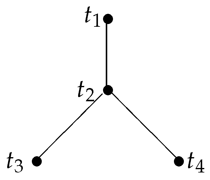
Example 1.

Let $S=\{l_{12},l_{23},l_{24}\}$ and $P=\{t_1,t_2,t_3,t_4\}$. $\oplus \left(P\right|S)$ is as follows (see Figure 3).

Definition 7.

Given a subnetwork $\oplus \left(P\right|S)$, if for any two different relations $t_i,t_j\in P$ there exist $t_{k_1},t_{k_2},\dots ,t_{k_m}\in P$ such that

$$t_i=t_{k_1},\oplus (t_{k_{𝓁}},t_{k_{𝓁+1}})\in S,t_{k_m}=t_j,$$

where $𝓁=1,2,\dots ,m-1$, then $\oplus \left(P\right|S)$ is called a relation chain. Moreover, $\oplus \left(P\right|S)$ is called a k-chain if $\left|P\right|=k$.

In particular, relations are 1-chains. In this paper, we only consider relation chains. A relation chain is not necessarily a path, as mentioned in traditional graph theory (see Example 1). In fact, relation chains are connected subnetworks. Compared with the 2-chain’s structures, the research of general relation chains is more macro and rich. Therefore, in the following, we focuse on the algebraic system consisting of relation chains. Obviously, the result obtained by joining two relation chains is still a relation chain, and thus the reducing of the set of 2-chains can be extended to any two relation chains as follows:

Definition 8.

For any two nonempty relation chains $l_1=\oplus \left(P_1\right|S_1)$ and $l_2=\oplus \left(P_2\right|S_2)$, the following applies:

$$l_1\mathring{\cup }{l}_2=\left\{\begin{array}{cc}\mathring{\cup }(S_1\cup S_2)\hfill & \mathrm{if}{P}_1\cap P_2\ne \varnothing \hfill \\ \varnothing \hfill & \mathrm{otherwise}.\hfill \end{array}\right.$$

The set of all nonempty relation chains generated by the relations in $T_{\Gamma }$ is called the universal set of relation chains of the network $\Gamma$, written as ${\oplus }_{\mathrm{all}}(t_1,t_2,\dots ,t_n)$. For convenience, $\mathcal{L}(\Gamma )$ denotes the union of ${\oplus }_{\mathrm{all}}(t_1,t_2,\dots ,t_n)$ and $\{\varnothing \}$, where ∅ is the empty relation; that is, $\mathcal{L}(\Gamma )={\oplus }_{\mathrm{all}}(t_1,t_2,\dots ,t_n)\cup \{\varnothing \}$. In the following, we show that $\mathcal{L}(\Gamma )$ forms a quasi-semilattice with respect to $\mathring{\cup }$.

Theorem 1.

For any general network Γ, $\mathcal{L}(\Gamma )$ forms a quasi-semilattice with respect to $\mathring{\cup }$, called a network quasi-semilattice.

Proof. 

It is easy to see that for any two elements $l_1,l_2\in \mathcal{L}(\Gamma )$, we have $l_1\mathring{\cup }{l}_2\in \mathcal{L}(\Gamma )$; that is, $\mathcal{L}(\Gamma )$ is closed with respect to $\mathring{\cup }$. Clearly, $\varnothing \oplus \varnothing =\varnothing$, and for any nonempty relation chain $l=\oplus \left(P\right|S)$, we have $l\mathring{\cup }l=\mathring{\cup }(S\cup S)=\mathring{\cup }S=l$. Thus, every element of $\mathcal{L}(\Gamma )$ is idempotent. Naturally, $\mathring{\cup }$ is commutative as the union of sets is commutative.

Now, we show that the associative law does not hold. Suppose that $l_1=\oplus \left(P_1\right|S_1)$, $l_2=\oplus \left(P_2\right|S_2)$ and $l_3=\oplus \left(P_3\right|S_3)$ are three nonempty elements of $\mathcal{L}(\Gamma )$ such that $P_1\cap P_2\ne \varnothing$, $P_1\cap P_3\ne \varnothing$ and $P_2\cap P_3=\varnothing$. From $P_1\cap P_2\ne \varnothing$, we have $l_1\mathring{\cup }{l}_2=\mathring{\cup }(S_1\cup S_2)\ne \varnothing$. Since $P_1\cap P_3\ne \varnothing$, it follows that $(P_1\cup P_2)\cap P_3\ne \varnothing$. Furthermore, $\left(l_1\mathring{\cup }{l}_2\right)\mathring{\cup }{l}_3=\mathring{\cup }(S_1\cup S_2)\mathring{\cup }{l}_3=\mathring{\cup }(S_1\cup S_2\cup S_3)\ne \varnothing$, while we have $l_2\mathring{\cup }{l}_3=\varnothing$ as $P_2\cap P_3=\varnothing$. Then, $l_1\mathring{\cup }\left(l_2\mathring{\cup }{l}_3\right)=l_1\mathring{\cup }\varnothing =\varnothing$. Hence, $\left(l_1\mathring{\cup }{l}_2\right)\mathring{\cup }{l}_3\ne l_1\mathring{\cup }\left(l_2\mathring{\cup }{l}_3\right)$, which implies that $\mathcal{L}(\Gamma )$ is non-associative with respect to $\mathring{\cup }$. □

5. Congruences on $\mathcal{L}(\Gamma )$

The purpose of this section is to define a congruence on $\mathcal{L}(\Gamma )$ and investigate its classes.

Naturally, there exist two natural ways to classify relation chains; one is with the number of relations generating a chain, and the other is the relations generating a chain. According to the two classification methods, we define two relations $\sigma$ and $\delta$ on $\mathcal{L}(\Gamma )$ as follows.

Definition 9.

For any $l_1=\oplus \left(P_1\right|S_1)$ and $l_2=\oplus \left(P_2\right|S_2)$ in $\mathcal{L}(\Gamma )$, the following are true:

(i) $(l_1,l_2)\in \sigma$ if $\left|P_1\right|=\left|P_2\right|$;

(ii) $(l_1,l_2)\in \delta$ if $P_1=P_2$.

The following lemma presents that $\sigma$ and $\delta$ are equivalences:

Lemma 1.

Relations σ and δ are equivalent relations on $\mathcal{L}(\Gamma )$.

Proof. 

Suppose that $l_1=\oplus \left(P_1\right|S_1)$, $l_2=\oplus \left(P_2\right|S_2)$ and $l_3=\oplus \left(P_3\right|S_3)$ are elements of $\mathcal{L}(\Gamma )$.

Now, we show that $\sigma$ is equivalent. $\left(1\right)$ For any $l=\oplus \left(P\right|S)\in \mathcal{L}(\Gamma )$, we have $(l,l)\in \sigma$ as $\left|P\right|=\left|P\right|$. Thus, $\sigma$ is reflexive. $\left(2\right)$ If $(l_1,l_2)\in \sigma$, then $\left|P_1\right|=\left|P_2\right|$, which implies that $(l_2,l_1)\in \sigma$. Thus, $\sigma$ is symmetric. $\left(3\right)$ If $(l_1,l_2)\in \sigma$ and $(l_2,l_3)\in \sigma$, then $\left|P_1\right|=\left|P_2\right|$ and $\left|P_2\right|=\left|P_3\right|$. Thus, we have $\left|P_1\right|=\left|P_3\right|$, from which it follows that $(l_1,l_3)\in \sigma$. Thus, $\sigma$ is transitive.

It can be seen that $\delta$ is reflexive as for any $l=\oplus \left(P\right|S)\in \mathcal{L}(\Gamma )$, we have $(l,l)\in \delta$ as $P=P$. If $(l_1,l_2)\in \delta$, then $P_1=P_2$, from which it follows that $(l_2,l_1)\in \delta$, and thus $\delta$ is symmetric. Suppose that $(l_1,l_2)\in \delta$ and $(l_2,l_3)\in \delta$. Then, $P_1=P_2$ and $P_2=P_3$, which implies that $P_1=P_3$, and thus $\delta$ is transitive. □

In $(\mathcal{L}(\Gamma ),\mathring{\cup })$, $\sigma$ is not a congruence as it is not compatible. Clearly, $\mathring{\cup }$ is commutative, and thus it is sufficient to show that $\sigma$ is not left compatible with respect to $\mathring{\cup }$. Let $l_1,l_2,l_3\in \mathcal{L}(\Gamma )$ be such that $(l_1,l_2)\in \sigma$, $l_3\mathring{\cup }{l}_1=\varnothing$ and $l_3\mathring{\cup }{l}_2\ne \varnothing$. As $(\varnothing ,l_3\mathring{\cup }{l}_2)\notin \sigma$, we obtain $(l_3\mathring{\cup }{l}_1,l_3\mathring{\cup }{l}_2)\notin \sigma$, from which it follows that $\sigma$ is not left compatible.

Lemma 2.

Relation δ is a congruence on $\mathcal{L}(\Gamma )$.

Proof. 

It is sufficient to show that $\delta$ is left compatible since $\delta$ is an equivalence with Lemma 1, and $\mathring{\cup }$ is commutative. Let $l_1=\oplus \left(P_1\right|S_1)$, $L_2=\oplus \left(P_2\right|S_2)$ and $l_3=\oplus \left(P_3\right|S_3)$ be elements of $\mathcal{L}(\Gamma )$ such that $(l_1,l_2)\in \delta$. Therefore, we have $P_1=P_2$, from which it follows that $P_1\cap P_3=P_2\cap P_3$. If $P_1\cap P_3=\varnothing$, then we have $(l_3\mathring{\cup }{l}_1,l_3\mathring{\cup }{l}_2)\in \delta$ as $l_3\mathring{\cup }{l}_1=l_3\mathring{\cup }{l}_2=\varnothing$, while if $P_1\cap P_3\ne \varnothing$, we find that $l_3\mathring{\cup }{l}_1=\mathring{\cup }(S_1\cup S_3)=\oplus (P_1\cup P_3|S_1\cup S_3)$ and $l_3\mathring{\cup }{l}_2=\mathring{\cup }(S_2\cup S_3)=\oplus (P_2\cup P_3|S_2\cup S_3)$. It follows from $P_1=P_2$ that $P_1\cup P_3=P_2\cup P_3$, and thus $(l_3\mathring{\cup }{l}_1,l_3\mathring{\cup }{l}_2)\in \delta$. □

Let $l_1=\oplus \left(P_1\right|S_1)$ and $l_2=\oplus \left(P_2\right|S_2)$ be elements of $\mathcal{L}(\Gamma )$ such that $\left|P_1\right|=\left|P_2\right|=k\in \mathbb{N}$. If $|P_1\cap P_2|=m(0<m<k)$, then we obtain a $2k-m$-chain $l_1\mathring{\cup }{l}_2$. If $P_1\cap P_2=\varnothing$, then we obtain $l_1\mathring{\cup }{l}_2=\varnothing$. Thus, in general, $\mathring{\cup }$ is impossible to be closed in a $\sigma$-equivalent class. Any two chains in the same $\delta$-equivalent class are generated by the same relations so that their reducing result is still in the same equivalent class. Thus, each $\delta$ class forms a subalgebra of $\mathcal{L}(\Gamma )$, but a $\sigma$ class is impossible to be a subalgebra of $\mathcal{L}(\Gamma )$.

Proposition 1.

Each δ class of $\mathcal{L}(\Gamma )$ is a subsemilattice of $\mathcal{L}(\Gamma )$ with respect to $\mathring{\cup }$.

Proof. 

Clearly, the $\delta$ class of the empty element ∅ only contains ∅, and thus it is a semilattice with respect to $\mathring{\cup }$.

For any nonempty element $l\in \mathcal{L}(\Gamma )$, if $l=\oplus \left(P\right|S)\in \mathcal{L}(\Gamma )$, then according to the definition of $\delta$, $l\delta$ consists of relation chains generated by P. Now, we show that $l\delta$ is a semilattice with respect to $\mathring{\cup }$. It is sufficient to show that $\mathring{\cup }$ is closed and associative in $l\delta$ as $\mathring{\cup }$ is commutative, and every element of $\mathcal{L}(\Gamma )$ is idempotent. It is easy to see that $\mathring{\cup }$ is closed in $l\delta$ because for any $l_1,l_2\in l\delta$ with $l_1=\oplus \left(P_1\right|S_1)$ and $l_2=\oplus \left(P_2\right|S_2)$, we have $P_1=P_2=P$, and thus $l_1\mathring{\cup }{l}_2=\oplus \left(P\right|S_1\cup S_2)\in l\delta$. To show that $\mathring{\cup }$ is associative in $l\delta$, suppose that $l_1=\oplus \left(P\right|S_1)$, $l_2=\oplus \left(P\right|S_2)$ and $l_3=\oplus \left(P\right|S_3)$ are elements of $l\delta$. As their relation sets of $l_1$, $l_2$ and $l_3$ are the same (i.e., P), then the relation set of their reducing result is still P, and we also have $\left(l_1\mathring{\cup }{l}_2\right)\mathring{\cup }{l}_3=\mathring{\cup }(S_1\cup S_2)\mathring{\cup }{l}_3=\mathring{\cup }(S_1\cup S_2\cup S_3)=l_1\mathring{\cup }\left(\mathring{\cup }(S_2\cup S_3)\right)=l_1\mathring{\cup }\left(l_2\mathring{\cup }{l}_3\right)$, which implies that $\mathring{\cup }$ is associative in $l\delta$. Consequently, $l\delta$ is a semilattice with respect to $\mathring{\cup }$. According to Definition 2, $l\delta$ is a subsemilattice of $\mathcal{L}(\Gamma )$. □

A $\sigma$ equivalence class of $\mathcal{L}(\Gamma )$ consisting of k relations is the set of all k-chains. Each k-chain only belongs to one $\delta$ class. Therefore, a $\sigma$ equivalence class with k relations is the disjoint union of all $\delta$ equivalence classes with k relations (i.e., the disjoint union of subsemilattices). The relationship between different $\delta$ equivalence classes in the same $\sigma$ equivalence class is discussed below.

Let $l_1=\oplus \left(P_1\right|S_1)$ and $l_2=\oplus \left(P_2\right|S_2)$ be two nonempty elements of $\mathcal{L}(\Gamma )$ with $\left|P_1\right|=k_1$ and $\left|P_2\right|=k_2$, and let $S_{P_1}$ and $S_{P_2}$ be the set of all 2-chains generated by $P_1$ and $P_2$, respectively; that is, let us have

$$S_{P_1}=\left\{l_{i_1{j}_1}\right|i_1,j_1=1,2,\dots ,k_1;i_1\ne j_1;l_{i_1{j}_1}\ne \varnothing \},$$

$$S_{P_2}=\left\{l_{i_2{j}_2}\right|i_2,j_2=1,2,\dots ,k_2;i_2\ne j_2;l_{i_2{j}_2}\ne \varnothing \}.$$

Proposition 2.

If $\left|P_1\right|=\left|P_2\right|$, $\left|S_{P_1}\right|=\left|S_{P_2}\right|$, and there exist two bijections $\theta :P_1\to P_2$ and $\tau :S_{P_1}\to S_{P_2}$ with $\tau \left(l_{i_1{j}_1}\right)=l_{\theta \left(i_1\right)\theta \left(j_1\right)}\in S_{P_2}$, then $l_1\delta$ and $l_2\delta$ are isomorphic semilattices with respect to $\mathring{\cup }$, where $l_1=\oplus \left(P_1\right|S_1)$ and $l_2=\oplus \left(P_2\right|S_2)$.

Proof. 

It follows from Proposition 1 that $l_1\delta$ and $l_2\delta$ are subsemilattices of $\mathcal{L}(\Gamma )$. Assume that $\left|P_1\right|=\left|P_2\right|$, $\left|S_{P_1}\right|=\left|S_{P_2}\right|$, and there exist two bijections $\theta :P_1\to P_2$ and $\tau :S_{P_1}\to S_{P_2}$ with $\tau \left(l_{i_1{j}_1}\right)=l_{\theta \left(i_1\right)\theta \left(j_1\right)}\in S_{P_2}$. Let $\eta :l_1\delta \to l_2\delta$ be a map for any $l=\oplus \left(P_1\right|S_l)\in l_1\delta$, $\eta \left(l\right)=\oplus \left(\theta \left(P_1\right)\right|\tau \left(S_l\right))$, where $\theta \left(P_1\right)=P_2$ and $\tau \left(S_l\right)=\left\{\tau \left(l_{i_1{j}_1}\right)\right|l_{i_1{j}_1}\in S_l\subseteq S_{P_1}\}$. Clearly, $\eta$ is well defined.

To show that $\eta$ is injective, we suppose that $l=\oplus \left(P_1\right|S_l)$ and $l^{\prime }=\oplus \left(P_1\right|S_{l^{\prime }})$ are two elements of $l_1\delta$ such that $\eta \left(l\right)=\eta \left(l^{\prime }\right)$. Then, $\mathring{\cup }\tau \left(S_l\right)=\mathring{\cup }\tau \left(S_{l^{\prime }}\right)$. Furthermore, under Definition 6 and its generalization on relation chains, we obtain that $\tau \left(S_l\right)=\tau \left(S_{l^{\prime }}\right)$. As $\tau :S_{P_1}\to S_{P_2}$ is a bijection, it follows that $S_l=S_{l^{\prime }}$, which implies that $l=l^{\prime }$.

Next, we show that $\eta$ is surjective for any $l^{″}\in l_2\delta$ with $l^{″}=\oplus \left(P_2\right|S_{l^{″}})$. Since $\tau :S_{P_1}\to S_{P_2}$ is a bijection, it follows that ${\tau }^{-1}\left(S_{l^{″}}\right)\subseteq S_{P_1}$. As the relation set generating 2-chains in $S_{l^{″}}$ is $P_2$, and $\theta :P_1\to P_2$ is a bijection, we obtain that $P_1$ is the relation set generating 2-chains in ${\tau }^{-1}\left(S_{l^{″}}\right)$, and thus $\mathring{\cup }{\tau }^{-1}\left(S_{l^{″}}\right)\in l_1\delta$ such that $\eta \left(\mathring{\cup }{\tau }^{-1}\left(S_{l^{″}}\right)\right)=l^{″}$.

Finally, we claim that $\eta$ is a homomorphism. For any two elements $l=\oplus \left(P_1\right|S_l)$ and $l^{\prime }=\oplus \left(P_1\right|S_{l^{\prime }})$ of $l_1\delta$, we have $\eta \left(l_1\mathring{\cup }{l}_2\right)=\eta (\oplus \left(P_1\right|S_l\cup S_{l^{\prime }})=\oplus \left(\theta \left(P_1\right)\right|\tau (S_l\cup S_{l^{\prime }}))=\mathring{\cup }(\tau (S_l\cup S_{l^{\prime }})=\oplus \left(P_2\right|\tau \left(S_l\right))\mathring{\cup }\oplus \left(P_2\right|\tau \left(S_{l^{\prime }}\right))=\eta \left(l\right)\mathring{\cup }\eta \left(l^{\prime }\right)$.

To sum up, $\eta :l_1\delta \to l_2\delta$ is an isomorphism. □

Here, $\delta$ is a congruence on $\mathcal{L}(\Gamma )$, and relation chains in the same $\delta$ class consist of the same relation set. Thus, if the intersection of the relation sets of two different $\delta$ classes is nonempty, then the reducing of two chains from two different $\delta$ classes belongs to a $\delta$ class whose relation set is the union of relation sets of the two different $\delta$ classes; otherwise, the reducing of two chains from the two different $\delta$ classes is the empty element ∅. This means that $\mathring{\cup }$ deduces a binary operation in the set of $\delta$ classes of $\mathcal{L}(\Gamma )$ as follows.

Let $\mathcal{L}(\Gamma )/\delta$ be the set of all the $\delta$ classes of $\mathcal{L}(\Gamma )$ (i.e., $\mathcal{L}(\Gamma )/\delta =\left\{l\delta \right|l\in \mathcal{L}(\Gamma )\}$). For any two elements $l_1\delta ,l_2\delta \in \mathcal{L}(\Gamma )/\delta$, we have

$$\left(l_1\delta \right)\ast \left(l_2\delta \right)=\left(l_1\mathring{\cup }{l}_2\right)\delta .$$

Naturally, we obtain the following Lemma 3.

Lemma 3.

The set $\mathcal{L}(\Gamma )/\delta$ forms a quasi-semilattice with respect to ∗, defined above.

Therefore, there is a map from $(\mathcal{L}(\Gamma ),\mathring{\cup })$ to $\left(\mathcal{L}\right(\Gamma )/\delta ,\ast )$. In the following, a homomorphism between two quasi-semilattices is used to describe the map.

Theorem 2.

The map $\chi :\mathcal{L}(\Gamma )\to \mathcal{L}(\Gamma )/\delta$ with $\chi \left(l\right)=l\delta$ for any $l\in \mathcal{L}(\Gamma )$ is an epimorphism.

Proof. 

It is clear that $\chi$ is surjective. For any $l_1,l_2\in \mathcal{L}(\Gamma )$, we have $\chi \left(l_1\right)\ast \chi \left(l_2\right)=l_1\delta \ast l_2\delta =\left(l_1\mathring{\cup }{l}_2\right)\delta =\chi \left(l_1\mathring{\cup }{l}_2\right)$. Thus, $\chi$ is a homomorphism. □

At the end of this section, we remark that given a general network $\Gamma$, $\mathcal{L}(\Gamma )$ consists of all the relation chains, and all the $\delta$ classes form a partition of $\mathcal{L}(\Gamma )$. Each $\delta$ class is a semilattice. $\mathcal{L}(\Gamma )$ is a joint union of semilattices. Each semilattice contains all of the model of the relation chains generated by the same relation set.

6. Order Relations

The operation $\mathring{\cup }$ on $\mathcal{L}(\Gamma )$ can induce an order relation ⪯ on $\mathcal{L}(\Gamma )$ as follows. For any $l_1,l_2\in \mathcal{L}(\Gamma )$, we define that

$$l_1⪯l_2\mathrm{if}{l}_1\mathring{\cup }{l}_2=l_2.$$

Proposition 3.

The relation ⪯ defined above is a partial order relation on $(\mathcal{L}(\Gamma ),\mathring{\cup })$.

Proof. 

(1) Clearly, ⪯ is reflective since for any $l\in \mathcal{L}(\Gamma )$, we have $l\mathring{\cup }l=l$.

(2) To show that ⪯ is anti-symmetric, assume that $l_1,l_2\in \mathcal{L}(\Gamma )$ are such that $l_1⪯l_2$ and $l_1\ne l_2$. Then, $l_1\mathring{\cup }{l}_2=l_2$. If $l_2⪯l_1$, then we have $l_2\mathring{\cup }{l}_1=l_1$. It follows from $\mathring{\cup }$ being commutative that $l_1=l_2\mathring{\cup }{l}_1=l_1\mathring{\cup }{l}_2=l_2$, which is a contradiction of $l_1\ne l_2$. Therefore, $l_2{l}_1$.

(3) Now, we show that ⪯ is transitive. Suppose that $l_1,l_2,l_3\in \mathcal{L}(\Gamma )$ are such that $l_1⪯l_2$ and $l_2⪯l_3$. Let $l_1=\oplus \left(P_1\right|S_1)$, $l_2=\oplus \left(P_2\right|S_2)$ and $l_3=\oplus \left(P_3\right|S_3)$. Since $l_1⪯l_2$, we find that $P_1\subseteq P_2$ and $S_1\subseteq S_2$. Also, since $l_2⪯l_3$, we find that $P_2\subseteq P_3$ and $S_2\subseteq S_3$. Then, we have $P_1\subseteq P_3$ and $S_1\subseteq S_3$, and furthermore, we obtain that $l_1\mathring{\cup }{l}_3=\mathring{\cup }(S_1\cup S_3)=l_3$; that is, $l_1⪯l_3$. □

Next, we discuss the local maximum and local minimum elements in a $\delta$ class by using the partial order relation ⪯ on $\mathcal{L}(\Gamma )$ defined above.

Definition 10.

A nonempty element $l\in \mathcal{L}(\Gamma )$ is called a local maximum element of $l\delta$ if for any $l^{\prime }\in l\delta$, we have $l^{\prime }⪯l$. A nonempty element $l\in \mathcal{L}(\Gamma )$ is called a local minimum element of $l\delta$ if for any $l^{\prime }\in l\delta$ with $l^{\prime }⪯l$, we obtain $l^{\prime }=l$.

Proposition 4.

Each δ class of $\mathcal{L}(\Gamma )$ contains a unique local maximum element.

Proof. 

If the $\delta$ class contains only ∅, then it is clear that ∅ is the unique local maximum element of $\varnothing \delta$. Let $l\in \mathcal{L}(\Gamma )$ be a nonempty chain with $l=\oplus \left(P\right|S)$. Then, every chain in $l\delta$ is generated by P. Let $S_P$ denote the set of all 2-chains generated by P. Then, for any $l^{\prime }\in l\delta$ with $l^{\prime }=\oplus \left(P\right|S_{l^{\prime }})$, we have $S_{l^{\prime }}\subseteq S_P$ and also $l^{\prime }\mathring{\cup }\left(\mathring{\cup }{S}_P\right)=\mathring{\cup }(S_{l^{\prime }}\cup S_P)=\mathring{\cup }{S}_P\in l\delta$, from which it follows that $l^{\prime }⪯\mathring{\cup }{S}_P$, and thus $\mathring{\cup }{S}_P$ is the local maximum element.

To show the uniqueness, suppose that $l^{″}=\oplus \left(P\right|S_{l^{″}})\in l\delta$ is another local maximum element. Then, $\mathring{\cup }{S}_P⪯l^{″}$; that is, $l^{″}\mathring{\cup }\left(\mathring{\cup }{S}_P\right)=l^{″}$, which means that $S_P\cup S_{l^{″}}=S_{l^{″}}$. Together with $S_{l^{″}}\subseteq S_P$, we obtain $S_{l^{″}}=S_P$, and thus $l^{″}=\mathring{\cup }{S}_P$. □

Before we show that each $\delta$ class of $\mathcal{L}(\Gamma )$ contains local minimum elements, we recall the notion of spanning trees. A spanning tree $\Delta$ of a connected simple correlation network $\Gamma$ is a subnetwork such that $V_{\Delta }=V_{\Gamma }$ and there exists only one path between any two vertices in $\Delta$. It is easy to see that $|T_{\Delta }|=|V_{\Delta }|-1$.

Proposition 5.

Each δ class of $\mathcal{L}(\Gamma )$ contains local minimum elements.

Proof. 

If the $\delta$ class contains only ∅, then it is clear that ∅ is the unique local minimum element of $\varnothing \delta$. Let $l\in \mathcal{L}(\Gamma )$ be a nonempty chain with $l=\oplus \left(P\right|S)$, where $P=\{t_1,t_2,\dots ,t_k\}.$ Then, each chain in $l\delta$ is generated by P. Each relation chain $\oplus \left(P\right|S)$ can be regarded as a simple correlation network ${\Gamma }_P$ whose set of vertices is P and whose set of edges is S. According to Definition 7, ${\Gamma }_P$ is connected, and thus it has spanning trees. Assume that $l_T$ is a spanning tree of ${\Gamma }_P$. Then, the set of vertices of $l_T$ is P, and its set of edges is denoted by $S_{l_T}$. Then, $l_T=\oplus \left(P\right|S_{1_T})\in l\delta$. If $l^{\prime }=\oplus \left(P\right|S_{l^{\prime }})\in l\delta$ is such that $l^{\prime }⪯l_T$, then $l^{\prime }\mathring{\cup }{l}_T=l_T$, from which it follows that $S_{l^{\prime }}\subseteq S_{l_T}$. Since $l_T$ is a spanning tree, it contains only $k-1$ edges; that is, $\left|S_{l_T}\right|=k-1$. Therefore, $\left|S_{l^{\prime }}\right|\le k-1$. But $l^{\prime }$ is a connected chain containing all the relations in P, and therefore $\left|S_{l^{\prime }}\right|\ge k-1$. Thus, we obtain that $\left|S_{l^{\prime }}\right|=k-1$. Hence, a spanning tree of ${\Gamma }_P$$l_T$ is a local minimum element. □

Let $l\in \mathcal{L}(\Gamma )$ be a nonempty chain with $l=\oplus \left(P\right|S)$, where $P=\{t_1,t_2,\dots ,t_k\}.$ Then, each chain in $l\delta$ is generated by P. Let $S_P$ denote the set of all 2-chains generated by P. Then, we can draw a simple correlation network ${\Gamma }_P$ whose sets of vertices and edges are P and $S_P$, respectively. Its Laplace matrix A is a $k\times k$ matrix whose element in the ith row and jth column is

$$a_{ij}=\left\{\begin{array}{cc}-1\hfill & \mathrm{if}i\ne j\mathrm{and}{l}_{ij}\ne \varnothing \hfill \\ \mathrm{deg}\left(t_i\right)\hfill & \mathrm{if}i=j,\hfill \end{array}\right.$$

where deg$\left(t_i\right)$ is the number of 2-chains generated by $t_i$, which is the degree of $t_i$ in ${\Gamma }_P$. Furthermore, according to the Matrix-Tree Theorem [21], it can be obtained that the number of local minimum elements in the $l\delta$ class is equal to det$A_0$, where $A_0$ is the submatrix removing the ith row and ith column of Laplace matrix A, in which i is an arbitrary element of the set $\{1,2,\dots ,k\}$.

7. Path Algebras

In this section, graph inverse semigroups, Leavitt path algebras and Cuntz–Krieger graph $C^{*}$-algebras are constructed in terms of relations with respect to chain addition. To accomplish this, only first-order logic networks are considered in this section.

We first recall the notion of graph inverse semigroups [14].

Let $\Gamma$ be a first-order logic network. ${\Gamma }^0$ denotes the set of vertices of $\Gamma$, where ${\Gamma }^1$ denotes the set of relations of $\Gamma$. For any $v\in {\Gamma }^0$, we regard v as a path of a length of zero (or a trivial path), $\mathbf{s}\left(v\right)=\mathbf{r}\left(v\right)=v$, ${\mathbf{s}}^{-1}\left(v\right)=\{e\in {\Gamma }^1:s\left(e\right)=v\}$, and the out-degree of a vertex v is $|{\mathbf{s}}^{-1}\left(v\right)|$, being the number of logic relations with a source v. For any $e\in {\Gamma }^1$, $e^{*}$ is the inverse of e such that $\mathbf{s}\left(e^{*}\right)=\mathbf{r}\left(e\right)$ and $\mathbf{r}\left(e^{*}\right)=\mathbf{s}\left(e\right)$. Let ${\left({\Gamma }^1\right)}^{*}$ be the set $\left\{e^{*}\right|e\in {\Gamma }^1\}$. Assume that ${\Gamma }^1\cap {\left({\Gamma }^1\right)}^{*}=\varnothing$. The graph inverse semigroup $I(\Gamma )$ of $\Gamma$ is the semigroup with a zero element o generated by ${\Gamma }^0\cup {\Gamma }^1\cup {\left({\Gamma }^1\right)}^{*}$, satisfying the following relations:

(I1)

For all $e\in {\Gamma }^0\cup {\Gamma }^1\cup {\left({\Gamma }^1\right)}^{*}$, $\mathbf{s}\left(e\right)e=e\mathbf{r}\left(e\right)=e$;

(I2)

For any $u,v\in {\Gamma }^0$ with $u\ne v$, $uv=o$;

(I3)

For any $e,f\in {\Gamma }^1$ with $e\ne f$, $e^{*}f=o$;

(I4)

For $e\in {\Gamma }^1$, $e^{*}e=\mathbf{r}\left(e\right)$.

Next, we show how to generate graph inverse semigroups through chain addition of relations.

For any two different relations $e_1$ and $e_2$ with $\mathbf{r}\left(e_1\right)=\mathbf{s}\left(e_2\right)$, the 2-chain $\oplus (e_1,e_2)$ generated by $e_1$ and $e_2$ is a directed path from $\mathbf{s}\left(e_1\right)$ to $\mathbf{r}\left(e_2\right)$, called a two-line chain, which is simply denoted by $\oplus \langle e_1,e_2\rangle$. Here, $\langle e_1,e_2\rangle$ reflects the direction of the chain $\oplus \langle e_1,e_2\rangle$, which is from $\mathbf{s}\left(e_1\right)$ to $\mathbf{r}\left(e_2\right)$. Therefore, $\oplus \langle e_1,e_2\rangle \ne \oplus \langle e_2,e_1\rangle$.

Let $p=e_1{e}_2\cdots e_k$ be a direct path. Then, we can rewrite p as

$$\oplus \langle e_1,e_2\rangle \mathring{\cup }\oplus \langle e_2,e_3\rangle \mathring{\cup }\cdots \mathring{\cup }\oplus \langle e_{k-1},e_k\rangle$$

in light of the reducing of 2-chains; that is, the adjacent same relations in $\oplus \langle e_1,e_2\rangle \oplus \langle e_2,e_3\rangle \cdots \cdots \oplus \langle e_{k-1},e_k\rangle$ are combined into one, and the rest of the relations remain unchanged. Hence, the path $p=e_1{e}_2\cdots e_k$ is a relation chain generated by relations $e_1,e_2,\dots ,e_k$ according to the 2-chain set $S=\{\oplus \langle e_i,e_{i+1}\rangle |i=1,2,\dots ,k-1\}$, and the contra-variant index of the relation in p is the covariant index of its subsequent relation.

Definition 11.

Let $P=\{e_1,e_2,\cdots ,e_k\}$, $S=\{\oplus \langle e_i,e_{i+1}\rangle |i=1,2,\dots ,k-1\}$. The relation chain $\oplus \left(P\right|S)$ is called a directed path if $\mathbf{r}\left(e_i\right)=\mathbf{s}\left(e_{i+1}\right)$, $i=1,2,\cdots ,k-1$. $\oplus \left(P\right|S)$ is simply denoted by $e_1{e}_2\cdots e_k$.

Only two-line chains are considered in directed paths. Therefore, in order to generate directed paths and further generate graph inverse semigroups, the conditions for the chain addition of two different relations in Definition 4 is extended to ${\Gamma }^0\cup {\Gamma }^1\cup {\left({\Gamma }^1\right)}^{*}$ as follows:

Definition 12.

For any $t,t_1,t_2\in {\Gamma }^0\cup {\Gamma }^1\cup {\left({\Gamma }^1\right)}^{*}$, we have

$$t_1\overline{\oplus }{t}_2=\left\{\begin{array}{cc}{t}_1\hfill & \mathrm{if}{t}_1\in {\Gamma }^0\cup {\Gamma }^1\cup {\left({\Gamma }^1\right)}^{,}{t}_2\in {\Gamma }^0\mathrm{and}\mathbf{r}\left(t_1\right)=\mathbf{s}\left(t_2\right)\hfill \\ t_2\hfill & \mathrm{if}{t}_1\in {\Gamma }^0,t_2\in {\Gamma }^0\cup {\Gamma }^1\cup {\left({\Gamma }^1\right)}^{*}\mathrm{and}\mathbf{r}\left(t_1\right)=\mathbf{s}\left(t_2\right)\hfill \\ t_1{t}_2\hfill & \mathrm{if}{t}_1,t_2\in Tor{t}_1,t_2\in {\left({\Gamma }^1\right)}^{*}\mathrm{or}{t}_1\in T,t_2\in {\left({\Gamma }^1\right)}^{*}\mathrm{and}\mathbf{r}\left(t_1\right)=\mathbf{s}\left(t_2\right)\hfill \\ \mathbf{r}\left(t_2\right)\hfill & \mathrm{if}{t}_1\in {\left({\Gamma }^1\right)}^{*},t_2\in {\Gamma }^1,t_1^{*}=t_2\hfill \\ \varnothing \hfill & \mathrm{otherwise},\hfill \end{array}\right.$$

$$\varnothing \overline{\oplus }t=t\overline{\oplus }\varnothing =\varnothing ,$$

where $t_1{t}_2=\oplus \langle t_1,t_2\rangle$.

Obviously, $\overline{\oplus }$ can be generalized to directed paths. For any $t_1,t_2,t_3\in {\Gamma }^0\cup {\Gamma }^1\cup {\left({\Gamma }^1\right)}^{*}$, if $t_1\overline{\oplus }{t}_2=t_1{t}_2$, then we define $t_1{t}_2\overline{\oplus }{t}_3=t_1\left(t_2\overline{\oplus }{t}_3\right)$. Hence, for any directed paths $t_{i_1}{t}_{i_2}\cdots t_{i_{m_1}}$ and $t_{j_1}{t}_{j_2}\cdots t_{j_{m_2}}$, we have

$$t_{i_1}{t}_{i_2}\cdots t_{i_{m_1}}\overline{\oplus }{t}_{j_1}{t}_{j_2}\cdots t_{j_{m_2}}=t_{i_1}{t}_{i_2}\cdots t_{i_{m_1-1}}(\cdots \left(\left(t_{i_m}\overline{\oplus }{t}_{j_1}\right)\overline{\oplus }{t}_{j_2}\right)\overline{\oplus }\cdots \overline{\oplus }{t}_{j_{m_2}}).$$

Lemma 4.

The semigroup $T(\Gamma )$ generated by ${\Gamma }^0\cup {\Gamma }^1\cup {\left({\Gamma }^1\right)}^{*}$ and the empty element ∅ together with $\overline{\oplus }$ is an inverse semigroup.

Proof. 

According to Definition 12, it is easy to see that the forms of elements of $T(\Gamma )$ are $p,p^{*},p{q}^{*}$, where p and q are directed paths generated by relations in ${\Gamma }^0\cup {\Gamma }^1$ such that $\mathbf{r}\left(p\right)=\mathbf{r}\left(q\right)$. Because $\mathbf{r}{\left(p\right)}_{\mathbf{r}\left(p\right)}^{\mathbf{r}\left(p\right)}\in {\Gamma }^0$, ${\left({\mathbf{r}\left(p\right)}_{\mathbf{r}\left(p\right)}^{\mathbf{r}\left(p\right)}\right)}^{*}={\mathbf{r}\left(p\right)}_{\mathbf{r}\left(p\right)}^{\mathbf{r}\left(p\right)}$, and thus under Definition 12, $p=p\overline{\oplus }{\mathbf{r}\left(p\right)}_{\mathbf{r}\left(p\right)}^{\mathbf{r}\left(p\right)}$, and $p^{*}={\mathbf{r}\left(p\right)}_{\mathbf{r}\left(p\right)}^{\mathbf{r}\left(p\right)}{p}^{*}$. It follows that there is only one element form in $T(\Gamma )$, and that is $p{q}^{*}$, where p and q are directed paths generated by relations in ${\Gamma }^0\cup {\Gamma }^1$ such that $\mathbf{r}\left(p\right)=\mathbf{r}\left(q\right)$.

For any $p{q}^{*},x{y}^{*}\in T(\Gamma )$, we have

$$p{q}^{*}\overline{\oplus }x{y}^{*}=\left\{\begin{array}{cc}pz{y}^{*}\hfill & \mathrm{if}x=qz\hfill \\ p{\left(yw\right)}^{*}\hfill & \mathrm{if}q=xw\hfill \\ \varnothing \hfill & \mathrm{otherwise},\hfill \end{array}\right.$$

where z and w are directed paths generated by the relations in ${\Gamma }^0\cup {\Gamma }^1$.

Next, we show that $\overline{\oplus }$ is associative in $T(\Gamma )$. Suppose that $p{q}^{*},x{y}^{*},g{h}^{*}\in T(\Gamma )$.

Case I: If $x=q{z}_1,g=y{z}_2$, then we have $\left(p{q}^{*}\overline{\oplus }x{y}^{*}\right)\overline{\oplus }g{h}^{*}=p{z}_1{y}^{*}\overline{\oplus }g{h}^{*}=p{z}_1{z}_2{h}^{*}$ and $p{q}^{*}\overline{\oplus }\left(x{y}^{*}\overline{\oplus }g{h}^{*}\right)=p{q}^{*}\overline{\oplus }x{z}_2{h}^{*}=p{q}^{*}q{z}_1{z}_2{h}^{*}=p{z}_1{z}_2{h}^{*}$, and thus $\left(p{q}^{*}\overline{\oplus }x{y}^{*}\right)\overline{\oplus }g{h}^{*}=p{q}^{*}\overline{\oplus }\left(x{y}^{*}\overline{\oplus }g{h}^{*}\right)$.

Case II: If $x=q{z}_1,y=g{w}_2$, then $\left(p{q}^{*}\overline{\oplus }x{y}^{*}\right)\overline{\oplus }g{h}^{*}=p{q}^{*}q{z}_1{y}^{*}\overline{\oplus }g{h}^{*}=p{z}_1{\left(g{w}_2\right)}^{*}g{h}^{*}=p{z}_1{\left(h{w}_2\right)}^{*}$ and $p{q}^{*}\overline{\oplus }\left(x{y}^{*}\overline{\oplus }g{h}^{*}\right)=p{q}^{*}\overline{\oplus }x{\left(g{w}_2\right)}^{*}g{h}^{*}=p{q}^{*}\overline{x}{\left(h{w}_2\right)}^{*}=p{q}^{*}q{z}_1{\left(h{w}_2\right)}^{*}=p{z}_1{\left(h{w}_2\right)}^{*}$, from which it follows that $\left(p{q}^{*}\overline{\oplus }x{y}^{*}\right)\overline{\oplus }g{h}^{*}=p{q}^{*}\overline{\oplus }\left(x{y}^{*}\overline{\oplus }g{h}^{*}\right)$.

Case III: If $q=x{w}_1,g=y{z}_2$, then $\left(p{q}^{*}\overline{\oplus }x{y}^{*}\right)\overline{\oplus }g{h}^{*}=p{\left(x{w}_1\right)}^{*}x{y}^{*}\overline{\oplus }g{h}^{*}=p{\left(y{w}_1\right)}^{*}y{z}_2{h}^{*}=p{w}_1^{*}{z}_2{h}^{*}$ and $p{q}^{*}\overline{\oplus }\left(x{y}^{*}\overline{\oplus }g{h}^{*}\right)=p{q}^{*}\overline{\oplus }x{y}^{*}y{z}_2{h}^{*}=p{\left(x{w}_1\right)}^{*}x{z}_2{h}^{*}=p{w}_1^{*}{z}_2{h}^{*}$, from which it follows that $\left(p{q}^{*}\overline{\oplus }x{y}^{*}\right)\overline{\oplus }g{h}^{*}=p{q}^{*}\overline{\oplus }\left(x{y}^{*}\overline{\oplus }g{h}^{*}\right)$.

Case IV: If $q=x{w}_1,y=g{w}_2$, then $\left(p{q}^{*}\overline{\oplus }x{y}^{*}\right)\overline{\oplus }g{h}^{*}=p{\left(g{w}_2{w}_1\right)}^{*}g{h}^{*}=p{w}_1^{*}{w}_2^{*}{h}^{*}=p{\left(h{w}_1{w}_2\right)}^{*}$ and $p{q}^{*}\overline{\oplus }\left(x{y}^{*}\overline{\oplus }g{h}^{*}\right)=p{q}^{*}\overline{\oplus }x{\left(g{w}_2\right)}^{*}g{h}^{*}=p{q}^{*}\overline{\oplus }x{\left(h{w}_2\right)}^{*}=p{\left(x{w}_1\right)}^{*}x{\left(h{w}_2\right)}^{*}=p{\left(h{w}_2{w}_1\right)}^{*}$, from which it follows that $\left(p{q}^{*}\overline{\oplus }x{y}^{*}\right)\overline{\oplus }g{h}^{*}=p{q}^{*}\overline{\oplus }\left(x{y}^{*}\overline{\oplus }g{h}^{*}\right)$.

Case V: Otherwise, we have $\left(p{q}^{*}\overline{\oplus }x{y}^{*}\right)\overline{\oplus }g{h}^{*}=p{q}^{*}\overline{\oplus }\left(x{y}^{*}\overline{\oplus }g{h}^{*}\right)=\varnothing$. Thus, $\overline{\oplus }$ is associative in $T(\Gamma )$.

Now, we show that the set of idempotents of $T(\Gamma )$ is a semilattice with respect to $\overline{\oplus }$. It is easy to see that for any $p{q}^{*}\in T(\Gamma )$, $p{q}^{*}\overline{\oplus }p{q}^{*}=p{q}^{*}$ if and only if $q^{*}p=\mathbf{r}{\left(p\right)}_{\mathbf{r}\left(p\right)}^{\mathbf{r}\left(p\right)}$, and this is true if and only if $p=q$. Therefore, the set of idempotents of $T(\Gamma )$ is as follows:

$$E\left(T(\Gamma )\right)=\left\{p{p}^{*}\right|pisadirectedpathgeneratedbytherelationsin{T}^0\cup T\}\cup \{\varnothing \}.$$

For any $p{p}^{*},q{q}^{*}\in E\left(T(\Gamma )\right)$, we have

$$p{p}^{*}\overline{\oplus }q{q}^{*}=\left\{\begin{array}{cc}p{p}^{*}\hfill & \mathrm{if}p=qz\hfill \\ q{q}^{*}\hfill & \mathrm{if}q=pw\hfill \\ \varnothing \hfill & \mathrm{otherwise},\hfill \end{array}\right.$$

Also, $p{p}^{*}\overline{\oplus }q{q}^{*}=q{q}^{*}\overline{\oplus }p{p}^{*}$. Hence, $E\left(T\right(\Gamma \left)\right)$ is a semilattice.

Finally, for any $p{q}^{*}\in T(\Gamma )$, $q{p}^{*}$ is an inverse of $p{q}^{*}$ since $p{q}^{*}\overline{\oplus }q{p}^{*}\overline{\oplus }p{q}^{*}=p{q}^{*}$ and $q{p}^{*}\overline{\oplus }p{q}^{*}\overline{\oplus }q{p}^{*}=q{p}^{*}$.

To sum up, $T(\Gamma )$ is an inverse semigroup. □

Proposition 6.

The map $\theta :I(\Gamma )\to T(\Gamma )$, defined by the rule that for any $e\in {\Gamma }^0\cup {\Gamma }^1\cup {\left({\Gamma }^1\right)}^{*}$, $\theta \left(e\right)=e$ and $\theta \left(o\right)=\varnothing$, is an isomorphism.

Proof. 

We first show that conditions (I1–I4) in the definition of graph inverse semigroups hold.

(I1) For any $e\in {\Gamma }^0\cup {\Gamma }^1\cup {\left({\Gamma }^1\right)}^{*}$, we have $\theta \left(\mathbf{s}\left(e\right)\right)\overline{\oplus }\theta \left(e\right)=\mathbf{s}\left(e\right)\overline{\oplus }e=e=\theta \left(e\right)$ and $\theta \left(e\right)\overline{\oplus }\theta \left(\mathbf{r}\left(e\right)\right)=e\overline{\oplus }\mathbf{r}\left(e\right)=e=\theta \left(e\right)$.

(I2) For any $u,v\in {\Gamma }^0$ with $u\ne v$, $\theta \left(u\right)\overline{\oplus }\theta \left(v\right)=u\overline{\oplus }v=\varnothing =\theta \left(o\right)$.

(I3) If $e,f\in {\Gamma }^1$ are such that $e\ne f$, then $\theta \left(e^{*}\right)\overline{\oplus }\theta \left(f\right)=e_{\mathbf{r}\left(e\right)}^{\mathbf{s}\left(e\right)}\overline{\oplus }f=\varnothing =\theta \left(o\right)$.

(I4) If $e\in {\Gamma }^1$, then $\theta \left(e^{*}\right)\overline{\oplus }\theta \left(e\right)=e_{\mathbf{r}\left(e\right)}^{\mathbf{s}\left(e\right)}\overline{\oplus }{e}_{\mathbf{s}\left(e\right)}^{\mathbf{r}\left(e\right)}=\mathbf{r}\left(e\right)=\theta \left(\mathbf{r}\left(e\right)\right)$.

Let $W={\Gamma }^0\cup {\Gamma }^1\cup {\left({\Gamma }^1\right)}^{*}$. Then, $\theta$ is a homomorphism from $I(\Gamma )=F_W/\sim$ to $T(\Gamma )$, where $F_W$ is the free semigroup over W and ∼ is the relation satisfying (I1–I4).

To show that $\theta$ is surjective, suppose that $p=e_1{e}_2\cdots e_k$ and $q=f_1{f}_2\cdots f_m$ are two directed paths are such that $\mathbf{r}\left(e_k\right)=\mathbf{r}\left(f_m\right)$. Then, we have

$$p{q}^{*}=e_1{e}_2\cdots e_k{f}_m^{*}\cdots f_2^{*}{f}_1^{*}.$$

Furthermore, we have

$$\theta (e_1{e}_2\cdots e_k{f}_m^{*}\cdots f_2^{*}{f}_1^{*})=\theta \left(e_1\right)\overline{\oplus }\theta \left(e_2\right)\overline{\oplus }\cdots \overline{\oplus }\theta \left(e_k\right)\overline{\oplus }\theta \left(f_m^{*}\right)\overline{\oplus }\cdots \overline{\oplus }\theta \left(f_2^{*}\right)\overline{\oplus }\theta \left(f_1^{*}\right)=p{q}^{*}.$$

Hence, $\theta$ is surjective. Obviously, it is injective, and thus $\theta$ is an isomorphism. □

Leavitt path algebras are derived from W.G. Leavitt’s seminal paper [22] and further studied in [18] and so on. Suppose that F is a field and the out-degree of each vertex in a first-order logic network $\Gamma$ is finite. The F-algebra generated by ${\Gamma }^0\cup {\Gamma }^1\cup {\left({\Gamma }^1\right)}^{*}$ and a zero element o is a Leavitt path algebra $L_F(\Gamma )$ if it satisfies relations (I1–I4) and the following Cuntz–Krieger relation (CK1).

CK1: $v={\sum }_{e\in {\mathbf{s}}^{-1}\left(v\right)}e{e}^{*}$ for any $v\in {\Gamma }^0$, and the out-degree of v is greater than zero.

If F is the complex field $\mathcal{C}$, then the Leavitt path algebra and Cuntz–Krieger graph $C^{*}$-algebra [17,19] are closely related. Suppose that ${\Gamma }^0$ and ${\Gamma }^1$ are countable and the out-degree of each vertex of $\Gamma$ is finite. The universal $C^{*}$-algebra is generated by ${\Gamma }^0\cup {\Gamma }^1\cup {\left({\Gamma }^1\right)}^{*}$, and a zero element o is a Cuntz–Krieger graph $C^{*}$-algebra $C^{*}(\Gamma )$ if it satisfies relations (I1–I4), (CK1) and the following:

CK2: For any $e\in {\Gamma }^1$, $e{e}^{*}\le \mathbf{s}\left(e\right)$.

Here, for any $u,v\in {\Gamma }^0$, $u\le v$ if there exists a path p such that $\mathbf{s}\left(p\right)=v$ and $\mathbf{r}\left(p\right)=u$; for any path $q=e_1{e}_2\dots e_k$ and $v\in {\Gamma }^0$, $q\le v$ if $\mathbf{r}\left(e_i\right)\le v$ for all $i\in 1,2,\dots ,k$.

Due to the proof of Proposition 6, the chain addition on $T^0$, T and $T^{*}$ satisfies (I1–I4) and thus according to the definition of Leavitt path algebras and Cuntz–Krieger graph $C^{*}$-algebras, except for the first-order logic network satisfying certain conditions, (The out-degree of each vertex is finite, and the sets of vertices and relations are countable.) only CK1 and CK2 need to be satisfied. Therefore, based on Definition 12, if CK1 and CK2 are satisfied, then Leavitt path algebras and Cuntz–Krieger graph $C^{*}$-algebras can be generated by ${\Gamma }^0$, ${\Gamma }^1$, ${\left({\Gamma }^1\right)}^{*}$ and ∅ with respect to the chain addition $\overline{\oplus }$.

8. Conclusions

Theorem 1 shows that all connected subnetworks of a network $\Gamma$ form a quasi-semilattice $\mathcal{L}(\Gamma )$. Graph inverse semigroups, Leavitt path algebras and Cuntz–Krieger graph $C^{*}$-algebras are algebraic systems of directed paths generated by relations of a first-order logic network. The network quasi-semilattice $\mathcal{L}(\Gamma )$ contains all connected subnetworks of a general network $\Gamma$. Therefore, the study of the algebraic structure of $\mathcal{L}(\Gamma )$ will help to study all the substructures (including paths) of a general network. In particular, with respect to the partial order relation ⪯ given in Section 6, the minimum elements of a congruence $\delta$ class, say $l\delta$ of $\mathcal{L}(\Gamma )$, are spanning trees generated by all relations of $l\delta$. It is helpful to detect spanning trees by investigating the minimum elements of classes of the congruence $\delta$.