Similarity Classes of the Longest-Edge Trisection of Triangles

Abstract

This paper studies the triangle similarity classes obtained by iterative application of the longest-edge trisection of triangles. The longest-edge trisection (3T-LE) of a triangle is obtained by joining the two points which divide the longest edge in three equal parts with the opposite vertex. This partition, as well as the longest-edge bisection (2T-LE), does not degenerate, which means that there is a positive lower bound to the minimum angle generated. However, unlike what happens with the 2T-LE, the number of similarity classes appearing by the iterative application of the 3T-LE to a single initial triangle is not finite in general. There are only three exceptions to this fact: the right triangle with its sides in the ratio 1:$\sqrt{2}$:$\sqrt{3}$ and the other two triangles in its orbit. This result, although of a combinatorial nature, is proved here with the machinery of discrete dynamics in a triangle shape space with hyperbolic metric. It is also shown that for a point with an infinite orbit, infinite points of the orbit are in three circles with centers at the points with finite orbits.

1. Introduction

It is well known that numerical mesh generation and adaptive meshing or local refinement of a given mesh are the main steps in many areas such as geometric modelling, computer graphics, or the finite element method (FEM). Also, the geometry of the generated elements is important for the numerical convergence of the method. The grid generation as well as a proper local refinement or coarsening strategies are of the most importance to find the solution strategy in these problems [1,2].

One of the possibilities to refine a given simplicial mesh is to employ some type of partition. Partitions of simplices, triangles, or tetrahedra have been studied profusely, and issuessuch as the non-degeneracy or stability condition as well as the conformity and the nestedness of the refined meshes are usually addressed [3,4,5,6].

For the longest-edge bisection of triangles, the non-degeneracy was proved by Rosenberg and Stenger [7] and similar results have been presented recently for the longest-edge trisection or in general for the longest n-section of triangles. See [8] and references therein.

The longest-edge trisection (3T-LE) of a triangle is obtained by joining the two equally spaced points of the longest-edge with the opposite vertex. The present note studies the triangle similarity classes that appear by the iterative application of the 3T-LE.

The 2T-LE of triangles has finite orbit always (see [9,10]). However, the number of similarity classes appearing by the iterative application of the 3T-LE to a single initial triangle is not finite in general. There are only three exceptions to this fact: the right triangle with side lengths proportional to 1:$\sqrt{2}$:$\sqrt{3}$ and the other two triangles in its orbit. In this paper, we prove this fact by the discrete dynamics in a space of triangular shapes endowed with hyperbolic distance.

2. Space of Triangular Shapes and the Hyperbolic Metric in the Space of Triangular Shapes

2.1. Normalized Triangle Region or Space of Triangular Shapes

Since only the shape of triangles will be taken into account here, it is very convenient to have a way to represent the shape of a triangle in a univocal and systematic way, in a subset of the complex plane.

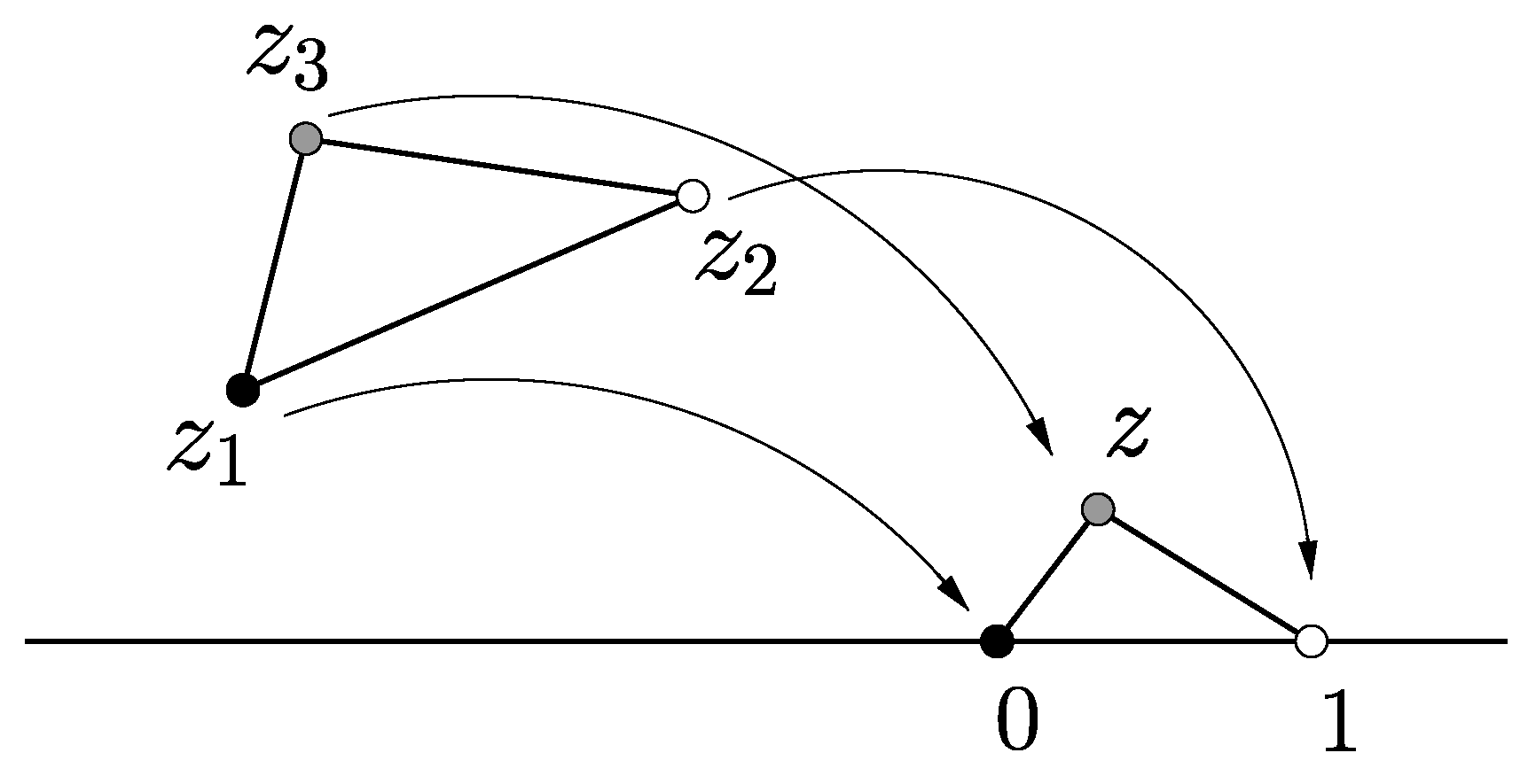
Let $z_1$, $z_2$, and $z_3$ be three points in the complex plane such that at least two of them are different. For example, let $z_1\ne z_2$. Then, the triangle with vertices $z_1$, $z_2$, and $z_3$ has the same shape as the triangle with vertices 0, 1, and $z=\frac{z_3-z_1}{z_2-z_1}$. The real part and imaginary part of complex z are called Bookstein’s coordinates [11,12]. See Figure 1.

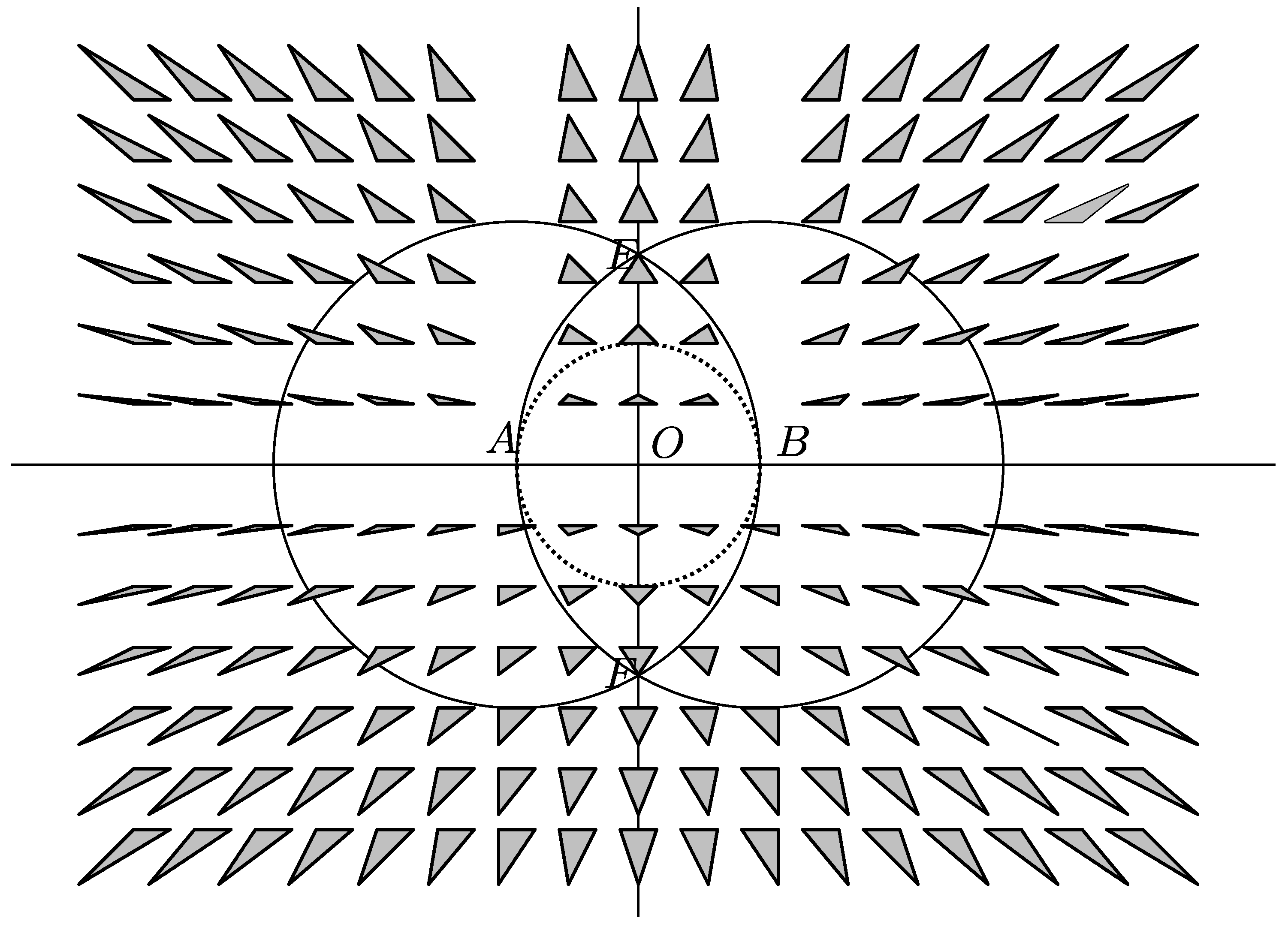
By means of Bookstein’s coordinates, we may use the complex plane as a space of triangular shapes. An idea of this space of triangular shapes is shown in Figure 2, where each triangle is drawn with its center of the base at the position corresponding to its Bookstein’s coordinates. See Figure 2, which is similar to the one given in [13].

In Figure 2, equilateral triangles correspond to points $\frac{1}{2}+\frac{\sqrt{3}}{2}i$ and $\frac{1}{2}-\frac{\sqrt{3}}{2}i$, points E and F in the Figure. Right triangles are located on the lines with equations $\mathrm{Re}z=0$ and $\mathrm{Re}z=1$ and on the circumference $\left|z-\frac{1}{2}\right|=\frac{1}{2}$. Isosceles triangles are on the line $\mathrm{Re}z=\frac{1}{2}$ and on the circumferences $\left|z\right|=1$ and $\left|z-1\right|=1$. Degenerate triangles have their vertices on the line $\mathrm{Im}z=0$.

The upper semiplane may be subdivided into six regions by the line $\mathrm{Re}z=\frac{1}{2}$ and the circumferences $\left|z\right|=1$ and $\left|z-1\right|=1$. Since the permutation of the vertices of any triangle does not change its shape, we may assign one point in each of these six regions of the upper plane.

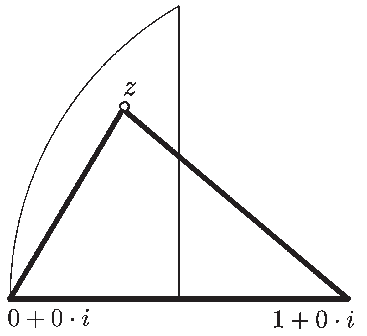
In order to achieve a bijective relation between any triangle shape and a point of a subset of the complex plane, we have to chose one of these regions as a normalized region. By using scaling, symmetries, translations, and rotations, we may associate with any given triangle a normalized triangle similar to the former one. This normalized triangle has the two vertices of the longest edge at points 0 and 1 of the real axes, and the opposite vertex to the longest edge on the upper half plane and on the left of the line $\mathrm{Re}z=\frac{1}{2}$. That is, the opposite vertex to the longest edge is in the set $\Sigma =\left\{z\in \mathbb{C}/\mathrm{Im}z>0,\mathrm{Re}z\le \frac{1}{2},|z-1|\le 1\right\}$. Then, there is a bijection between the points in $\Sigma$ and the classes of similar triangles. $\mathrm{Re}z=\frac{1}{2}$.

Region $\Sigma$ is called here the normalized region or space of triangular shapes. See Figure 3.

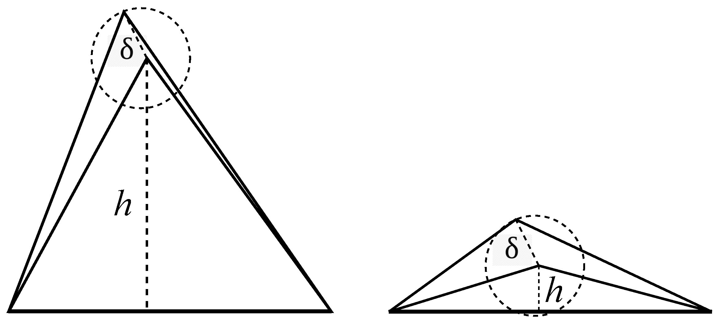
2.2. Introduction to the Hyperbolic Metric in the Space of Triangular Shapes

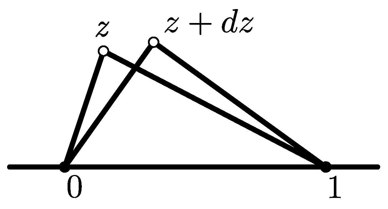
Let us consider on one hand two triangles both with Bookstein’s coordinates close to the real axis and at a Euclidean distance $\delta$. On the other hand, let us consider two other triangles with Bookstein’s coordinates at the same Euclidean distance $\delta$ but far away from the real axis. The same Euclidean distance $\delta$ is less important when the distance to the real axis grows h; it is understandable to consider the hyperbolic distance between points representing triangular shapes [13]. See Figure 4.

A more formal justification of the election of the hyperbolic distance may be found in [14] and may be extended to higher dimensions.

Let $z=z_1+z_{2}i$ and $w=w_1+w_{2}i$ in the upper semiplane of the respective Bookstein’s coordinates of two triangles. The affine transformation applying 0, 1, z, respectively, to 0, 1, w is a linear transformation, which may be written as a product of a column vector by the upper triangular matrix

$$\Lambda =\left(\begin{array}{cc}1& \frac{w_1-z_1}{z_2}\\ 0& \frac{w_2}{z_2}\end{array}\right).$$

If w is a small perturbation of z, then $w=z+dz$, with $w_1=z_1+d{z}_1$, and $w_2=z_2+d{z}_2$. See Figure 5.

In that case, matrix $\Lambda$ may be written as $I+d\Lambda$, where I is the $2\times 2$ identity matrix and

$$d\Lambda =\frac{1}{z_2}\left(\begin{array}{cc}0& d{z}_1\\ 0& d{z}_2\end{array}\right).$$

In order to find the eigenvalues of $\Lambda$, we find first the eigenvalues of ${\Lambda }^T\Lambda$. Since $\Lambda$ is a perturbation of the identity matrix, it follows that

$${\left(I+d\Lambda \right)}^T\left(I+d\Lambda \right)\approx I+d{\Lambda }^T+d\Lambda ,$$

after canceling less significant terms. Using the last expression, the characteristic equation for the eigenvalues is written as

$$\det \left(\lambda I-\left(I+d{\Lambda }^T+d\Lambda \right)\right)=0.$$

The last equation is of the second degree in $\lambda$. The eigenvalues ${\lambda }_1$ and ${\lambda }_2$ of ${\Lambda }^T\Lambda$ are the two roots of this equation and may be found explicitly as

$$1+\frac{d{z}_2\pm \sqrt{d{z}_1^2+d{z}_2^2}}{z_2}.$$

(1)

Let ${\lambda }_1$ be the largest eigenvalue and ${\lambda }_2$ be the smallest one. Since z is in the upper upper plane, coordinates $z_2>0$. Therefore, ${\lambda }_1$ corresponds to the sign + and ${\lambda }_2$ to the sign − in expression (1). Considering ${\lambda }_1$ and ${\lambda }_2$ infinitesimal variations of the unity, they may be written as ${\lambda }_1\approx 1+d{\lambda }_1$ and ${\lambda }_2\approx 1+d{\lambda }_2$.

The eigenvalues of $\Lambda$ are the square roots of the eigenvalues of ${\Lambda }^T\Lambda$. They are also perturbations of the unity that may be written as

$$\alpha \approx \sqrt{1+d{\lambda }_1}\approx 1+\frac{d{\lambda }_1}{2} \mathrm{and} \beta \approx \sqrt{1+d{\lambda }_2}\approx 1+\frac{d{\lambda }_2}{2},$$

and therefore, ${\displaystyle ln\left(\frac{\alpha }{\beta }\right)\approx \frac{d{\lambda }_1}{2}-\frac{d{\lambda }_2}{2}.}$ By using the expression of ${\lambda }_1$ and ${\lambda }_2$, it is obtained that the infinitesimal distance between two points with Bookstein’s coordinates z and $z+dz$ is given by

$${\displaystyle ds=\frac{\sqrt{d{z}_1^2+d{z}_2^2}}{z_2},}$$

which may be recognized as the expression for the hyperbolic metric for the Poincare plane.

2.3. Poincare Model the the Hyperbolic Plane

Let $\mathbb{H}=\left\{z\in \mathbb{C}\mathrm{such}\mathrm{that}\mathrm{Im}z>0\right\}$ is the upper semi-plane. Here, the distance is defined by ${\displaystyle d{s}^2=\frac{d{x}^2+d{y}^2}{y^2}}$. For a continuous curve $\gamma :[a,b]\to \mathbb{H}$ given by $\gamma \left(t\right)=({\gamma }_1\left(t\right),{\gamma }_2\left(t\right))$, its length with this metric is given by

$${\displaystyle \ell \left(\gamma \right)={\int }_a^b\frac{\sqrt{\left({\gamma }_1^{\prime }{\left(t\right)}^2\right)+\left({\gamma }_2^{\prime }{\left(t\right)}^2\right)}}{{\gamma }_2\left(t\right)}dt.}$$

The hyperbolic distance between $z_1$ and $z_2$ is defined as the minimum of the lengths of all paths joining points $z_1$ and $z_2$:

$$d(z_1,z_2)=inf\left\{\ell \left(\gamma \right)/\gamma :[a,b]\to \mathbb{H},\gamma \left(a\right)=z_1,\gamma \left(b\right)=z_2\right\}.$$

The last expression has all the properties of a distance in $\mathbb{H}$, and $d(z_1,z_2)=ln\left(\frac{b}{a}\right)$. Note that the semi-line ${\gamma }^{*}\left(t\right)=x+ti$ for $0<t<\infty$ holds the distance between any two of its points.

A curve that covers the minimum distance between any of its points is called a geodesic curve. A transformation $T:\mathbb{H}\to \mathbb{H}$ of the semi-plane $\mathbb{H}$ into itself is said to be an isometry if it preserves the hyperbolic metric.

In the Poincare semi-plane, the geodesic lines or hyperbolic lines are the semi-lines and the semi-circumferences that are the intersection with $\mathbb{H}$ of lines and circumferences orthogonal to the line $\mathrm{Im}z=0$.

3. Complex Functions Associated with the 3T-LE in the Space of Triangular Shapes

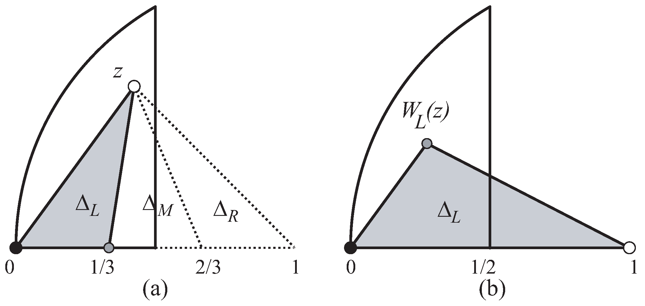
Definition 1.

Let Δ be a normalized triangle with associated point $z\in \Sigma$. By the 3T-LE partition applied to triangle Δ, three triangles are obtained. These triangles are called the left, middle, and right triangle. The left triangle ${\Delta }_L$ is the triangle with vertices 0, $\frac{1}{3}$, and z. The middle triangle ${\Delta }_M$ is the triangle with vertices $\frac{1}{3}$, $\frac{2}{3}$, and z. Finally the right triangle ${\Delta }_R$ is the triangle with vertices $\frac{2}{3}$, 1, and z.

Definition 2.

The normalization of the triangle ${\Delta }_L$ gives a complex number $W_L\left(z\right)\in \Sigma$. (see Figure 6). A complex function can be defined if this complex number is associated with z. In this way, left function $W_L$ is defined as the function of the region Σ into itself with $z\mapsto W_L\left(z\right)$, where z is the complex number associated with the initial triangle Δ. Functions $W_M$ and $W_R$ are associated, respectively, with ${\Delta }_M$ and ${\Delta }_R$ and are defined similarly.

Figure 6a shows the 3T-LE of a triangle where the left triangle ${\Delta }_L$ is in gray, and Figure 6b shows triangle ${\Delta }_L$ and $W_L\left(z\right)$.

In this way, the normalization process reduces the LE-trisection method to the discrete dynamic in the space of triangles $\Sigma$ associated with the three complex functions $W_L$, $W_M$, and $W_R$.

For the sake of completeness, the next Propositions show the boundaries for the subsets where functions $W_L$, $W_M$, and $W_R$ are defined as well as their explicit expressions in each subset. The different expressions for the piecewise functions $W_L$, $W_M$, and $W_R$ depend on the relative position of the longest edge on each triangle.

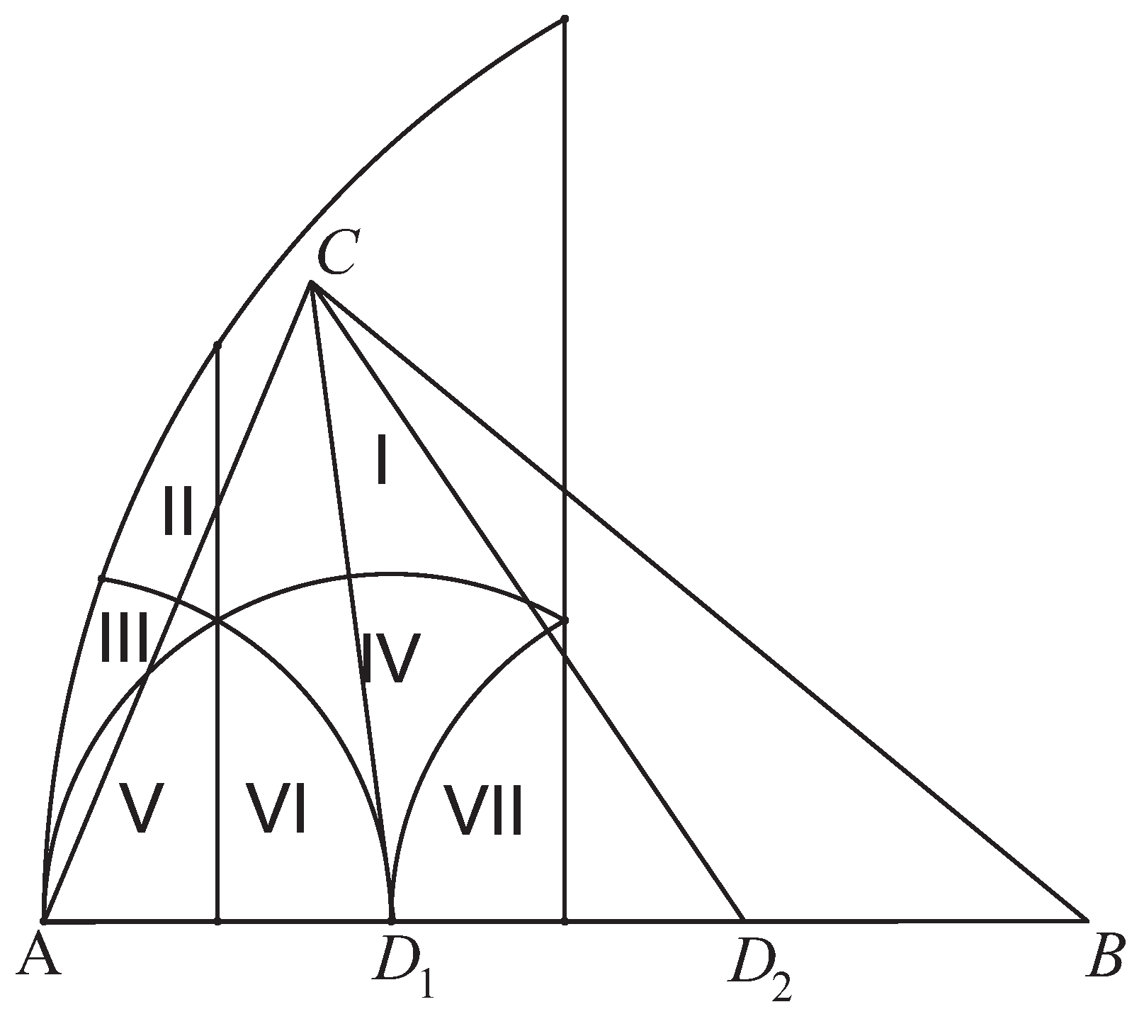
Proposition 1.

The boundary lines for the subregions of Σ, where functions $W_L$, $W_M$, and $W_R$ are defined, are straight line $Rez=\frac{1}{6}$ and circular arcs $\left|z\right|=\frac{1}{3}$, $\left|z-\frac{1}{3}\right|=\frac{1}{3}$, and $\left|z-\frac{2}{3}\right|=\frac{1}{3}$.

Proof. 

These regions depend on the relative position of the edges of triangles ${\Delta }_L$, ${\Delta }_M$ y ${\Delta }_R$ according to their length. The different possibilities are shown in Figure 7 and

Table 1. Metric relations between the three edges of the triangle according to the location of the opposite vertex to the longest-edge in each of the regions given in Figure 7.

I	$1/3AB\le C{D}_1$, $C{D}_1\le AC$, $C{D}_1\le C{D}_2$
II	$1/3AB\le AC\le C{D}_1\le C{D}_2$
III	$AC\le 1/3AB\le C{D}_1\le C{D}_2$
IV	$C{D}_1\le 1/3AB\le AC$, $1/3AB\le C{D}_2$
V	$AC\le C{D}_1\le 1/3AB\le C{D}_2$
VI	$C{D}_1\le AC\le 1/3AB\le C{D}_2$
VII	$C{D}_1\le C{D}_2\le 1/3AB\le AC$

. □

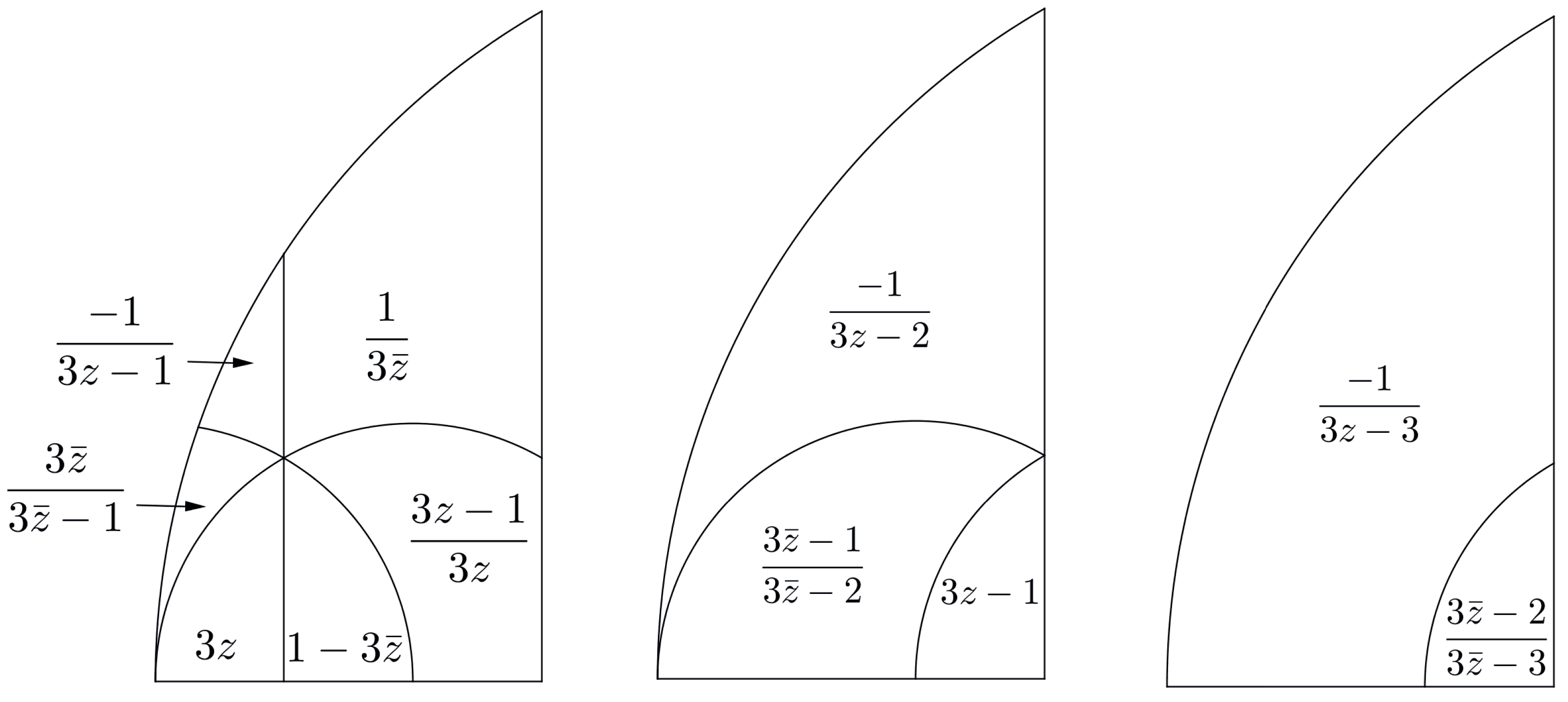
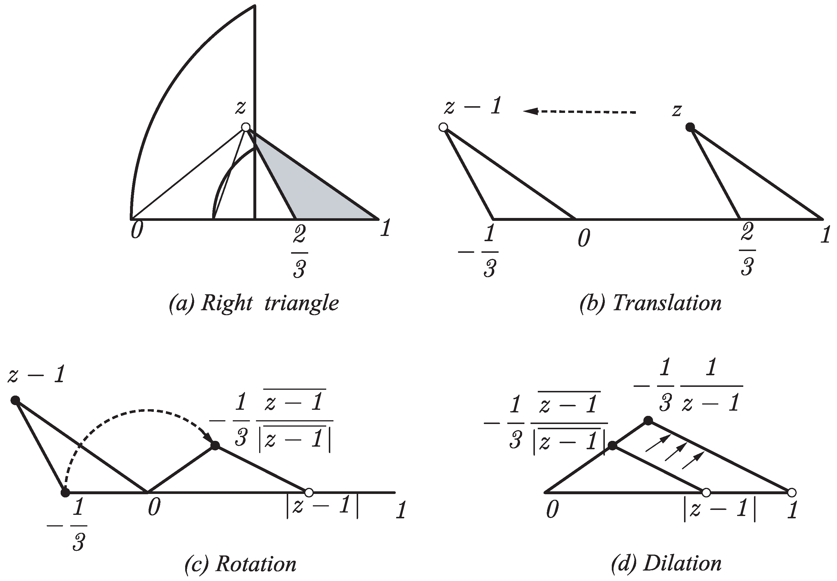
Proposition 2.

The different expressions for the piecewise functions $W_L$, $W_M$, and $W_R$ are as shown in Figure 8.

It should be noted that the expressions in Figure 8 are isometries in the Poincare semi-plane model for the hyperbolic plane.

Figure 9 shows how to deduce the expression of $W_R$ for a point z belonging to the upper subregion given in Figure 8. In order to normalize the right triangle in gray in Figure 9a, we apply first a translation in Figure 9b, then a rotation such that the longest edge of the rotated triangle is on the opposite real axes in Figure 9c and finally a dilation such that the longest edge is on segment $[0,1]$ in Figure 9d. The last expression is the value $W_R\left(z\right)=\frac{-1}{3z-3}$.

Proposition 3.

Let W be any of the functions $W_L$, $W_M$, and $W_R$. Then, W is invariant about the reflections with respect to the geodesic lines which appear in its definition.

Proof. 

These lines are geodesics according to the Poincare half-plane model for the hyperbolic plane. We may talk therefore about reflection with respect to these lines, taking into account that it means inversion in the case of a circumference or symmetry in the case of a right line. □

4. Discrete Dynamic of the 3T-LE Partition in the Space of Triangles $\Sigma$

Definition 3.

Let $z\in \Sigma$. The set of complex numbers obtained by iterative application of functions $W_L$, $W_M$, and $W_R$ to z and its successors is named orbit of z by the 3T-LE partition, and it is denoted by ${\Gamma }_z$. The cardinal of ${\Gamma }_z$ will be denoted by $\left|{\Gamma }_z\right|$.

We will show in this section that there are exactly three points in the space of triangular shapes with finite orbits. In addition, any other point will have an infinite orbit with infinite points in three circles with centers at the points with finite orbits.

Proposition 4.

If ${\omega }_1=\frac{1}{3}+\frac{\sqrt{2}}{3}i$, then its orbit is ${\Gamma }_{{\omega }_1}=\left\{{\omega }_1,{\omega }_2,{\omega }_3\right\}$, where ${\omega }_2=\frac{1}{3}+\frac{\sqrt{2}}{6}i$ and ${\omega }_3=\frac{4}{9}+\frac{\sqrt{2}}{9}i$.

Proof. 

It follows easily since $W_L\left({\omega }_1\right)={\omega }_1$, $W_M\left({\omega }_1\right)={\omega }_1$, $W_R\left({\omega }_1\right)={\omega }_2$, $W_L\left({\omega }_2\right)={\omega }_1$, $W_M\left({\omega }_2\right)={\omega }_1$, $W_R\left({\omega }_2\right)={\omega }_3$, $W_L\left({\omega }_3\right)={\omega }_2$, $W_M\left({\omega }_3\right)={\omega }_1$, and $W_R\left({\omega }_3\right)={\omega }_3$. □

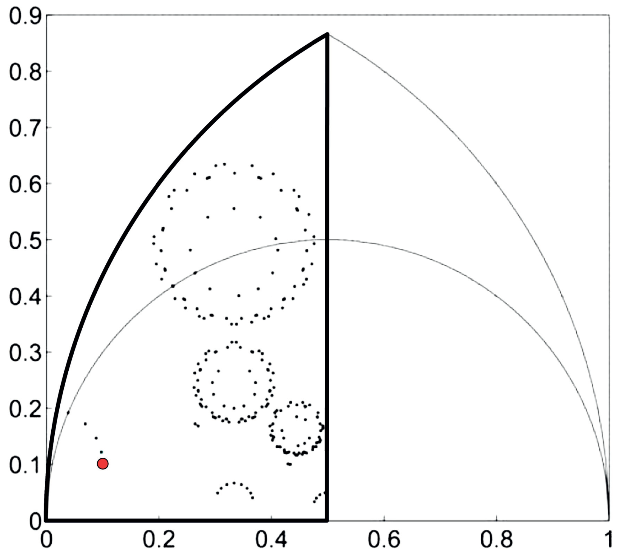
The orbits of points ${\omega }_1,{\omega }_2$, and ${\omega }_3$ are finite. These points correspond to the three shapes of the triangles obtained from the standard paper size by 3T-LE. Any other orbit has typical aspect showed in Figure 10: every point of the orbit is in circles around $\left\{{\omega }_1,{\omega }_2,{\omega }_3\right\}$, except perhaps a finite number of points.

Some facts about the Poincare semi-plane model and the hyperbolic geometry are naturally related to the discrete dynamic in the space of triangular shapes. See, for example, [15,16,17]. Here, d is the Poincare hyperbolic distance in the semi-plane:

Definition 4.

Let $z_1$ and $z_2$ be two points in the half-plane. Then, the hyperbolic distance between them, $d(z_1,z_2)$, is defined by the expression

$$coshd=1+\frac{|z_1-z_2{|}^2}{2·\mathit{Im}{z}_1·\mathit{Im}{z}_2}.$$

(2)

Our next goal is to prove that points ${\omega }_1,{\omega }_2$, and ${\omega }_3$ are the only ones with finite orbits. One interesting property of functions $W_L$, $W_M$, and $W_R$ is the non-increasing property as the following lemma establishes. For a proof of it, see [18].

Lemma 1.

Let $z_1,z_2\in \Sigma$ and let W be $W_L$, $W_M$, or $W_R$. Then, $d(W\left(z_1\right),W\left(z_2\right))\le d(z_1,z_2)$.

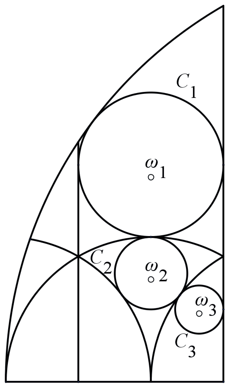
Proposition 5.

Circumferences $C_1$, $C_2$, and $C_3$, respectively, of equations

$$\begin{array}{ccc}\hfill C_1& \equiv & {\left(x-\frac{1}{3}\right)}^2+{\left(y-\frac{1}{2}\right)}^2={\left(\frac{1}{6}\right)}^2,\hfill \\ \hfill C_2& \equiv & {\left(x-\frac{1}{3}\right)}^2+{\left(y-\frac{1}{4}\right)}^2={\left(\frac{1}{12}\right)}^2,\hfill \\ \hfill C_3& \equiv & {\left(x-\frac{4}{9}\right)}^2+{\left(y-\frac{1}{6}\right)}^2={\left(\frac{1}{18}\right)}^2\hfill \end{array}$$

have centers, respectively, as the points ${\omega }_1=\frac{1}{3}+\frac{\sqrt{2}}{3}i$, ${\omega }_2=\frac{1}{3}+\frac{\sqrt{2}}{6}i$, ${\omega }_3=\frac{4}{9}+\frac{\sqrt{2}}{9}i$. These circumferences have radius $ln\sqrt{2}$ with the hyperbolic distance, and they are tangent to the boundary lines of the regions defining functions $W_L$, $W_M$, and $W_R$.

Proof. 

The proof follows by the definition of hyperbolic distance. See Figure 11. For example, in circumference $C_1$, the points at maximum and minimum height, respectively, are $\frac{1}{3}+\frac{2}{3}i$, and $\frac{1}{3}+\frac{1}{3}i$. Therefore, according to the formula for the hyperbolic distance (2), and the diameter of circumference $C_1$ is $D=ln2$. Let ${\omega }_1=\frac{1}{3}+yi$ be the center of circumference $C_1$. Then, the radius will be given by $r=ln\left(\frac{y}{2/3}\right)=\frac{1}{2}ln2$, and hence, $y=\frac{\sqrt{2}}{3}$, so effectively ${\omega }_1$ is as in the proposition. Analogously, the radius and center for circumferences $C_2$ and $C_3$ may be deduced. Notice that circumferences $C_1$, $C_2$, and $C_3$ may be written with the hyperbolic distance as $d(z,{\omega }_i)=\ln 2$, respectively, for $i=1,2,3$. □

Lemma 2

([19] (page 40)). $arccos\left(\frac{1}{\sqrt{n}}\right)$ is not a rational multiple of π for any odd number $n\ge 3$.

The following proposition explains the characteristic circular formations of the orbits of the 3T-LE.

Proposition 6.

Let $\omega \in \Sigma$ with $0<d(\omega ,{\omega }_i)=r<\ln \sqrt{2}$ for some $i\in \left\{1,2,3\right\}$. Then, the orbit of ω, ${\Gamma }_{\omega }$, is dense in any circumference $d(z,{\omega }_i)=r$ for $i=1,2,3$.

Proof. 

$W_L$, $W_M$, and $W_R$ interchange the hyperbolic circles with radius $\ln \sqrt{2}$ and centers ${\omega }_i$ for $i\in \left\{1,2,3\right\}$, or they are hyperbolic rotations in these circles. These rotations are not rational multiples of $2\pi$, and then any point $\omega$, as in the hypothesis, has an orbit dense in the circumferences $d(z,{\omega }_i)=r$ for $i=1,2,3$. Notice that function $W_M$ is given by ${\displaystyle \frac{-1}{3z-2}}$, which corresponds to an hyperbolic rotation with center ${\omega }_1$. Since the derivative of $W_M$ at ${\omega }_1$ is ${\displaystyle \frac{-1}{3}+\frac{2\sqrt{2}}{3}i}$, the angle of the hyperbolic rotation is ${\displaystyle \alpha =\frac{\pi }{2}+arctan\left(\frac{1}{2\sqrt{2}}\right)}$. Because $\tan \alpha =-2\sqrt{2}$, ${\displaystyle \cos (\pi -\alpha )=\frac{1}{3}}$, $\pi -\alpha$ is not a rational multiple of $\pi$, because of Lemma 2 for $n=9$ and also $\alpha$ is not a rational multiple of $\pi$.

Since $\alpha$ is not a rational multiple of $\pi$, if $m\ne n$, then $W_M^n\left(\omega \right)\ne W_M^m\left(\omega \right)$. Therefore, the orbit $\Gamma \left(\omega \right)$ is not finite. However, our goal is to prove that the orbit is dense in the hyperbolic circle with center ${\omega }_1$ and radius r. Let L be the hyperbolic length of that circle, and let z be such that $d(z,{\omega }_1)=r$. We have to prove that for every $\epsilon >0$ there is a point in $\Gamma \left(\omega \right)$ such that its hyperbolic distance to z is less than $\epsilon$. Let $N>0$ such that $1/N<\epsilon$. Let us consider the points $\omega ,W_M\left(\omega \right),W_M^w\left(\omega \right),\dots ,W_M^N\left(\omega \right)$, which are all different. Since they are $N+1$ points, two of them are in a hyperbolic circular arc of length $L/N$. It follows that there exist $0\le m<n\le N$ such that $d(W_M^n\left(\omega \right),W_M^m\left(\omega \right))<L/N<\epsilon$. Therefore, the points $\omega ,W_M\left(\omega \right),W_M^w\left(\omega \right),\dots ,W_M^N\left(\omega \right)$ are on a circle to a distance less than $\epsilon$ each from the following because $W_M$ is an isometry. Hence, there exists $j>0$ such that $d(z,W_M^{j(n-m)}\left(\omega \right))<\epsilon$. □

Proposition 7.

Let $z\in \Sigma$ with $\left|\Gamma \left(z\right)\right|<\infty$. Then, $z={\omega }_i$ for some $i\in \left\{1,2,3\right\}$.

Proof. 

Since the orbit $\Gamma \left(z\right)$ is finite, the sequence $z,W_M\left(z\right),W_M^2\left(z\right),\dots$ is cyclic, so there exist N and p such that $W_M^k\left(z\right)=W_M^{k+p}\left(z\right)$ for $k\ge N$. If $p=1$, then $W_M^k\left(z\right)$ is a point belonging to the subset of $\Sigma$ invariant by $W_M$, so $z={\omega }_1$. Let us suppose that $p\ge 2$, and p is the lower integer with that property. Let $y_j=W_M^{k+j-1}\left(z\right)$ for $j=1,\dots ,p$ different points. By the non-increasing property of the distance

$$d(y_1,{\omega }_1)\le d(y_2,{\omega }_1)\le \dots \le d(y_p,{\omega }_1)\le d(y_1,{\omega }_1).$$

Then,

$$d(y_1,{\omega }_1)=d(y_2,{\omega }_1)=\dots =d(y_p,{\omega }_1).$$

Therefore, $y_1,y_2,\dots ,y_p$ are in the same region of definition of $W_M$ where there is ${\omega }_1$. In that region, $W_M\left(z\right)=\frac{-1}{3z-2}$, which is a hyperbolic rotation with center ${\omega }_1$ and angle $\alpha =\frac{\pi }{2}+arctan\left(\frac{1}{2\sqrt{2}}\right)$ as in Proposition 6. But then $\alpha$ is not a rational multiple of $\pi$ which is a contradiction. Hence, there is an integer N such that $W_M^N\left(z\right)={\omega }_1$. Let us consider the lower N with that property. If $N=0$ or $N=1$, then by using the expression of $W_M$ it follows that $z={\omega }_i$ for some $i\in \left\{1,2,3\right\}$. Let us assume that $N\ge 2$. Then, either $W_M^{N-1}\left(z\right)={\omega }_2$ or $W_M^{N-1}\left(z\right)={\omega }_3$.

If $W_M^{N-1}\left(z\right)={\omega }_2$, then its pre-image $W_M^{N-2}\left(z\right)$ by $W_M$ is either $\frac{4}{9}+\frac{\sqrt{2}}{18}i$ or $\frac{2}{9}+\frac{\sqrt{2}}{9}i$. In both cases, it is not possible that the orbit is finite, because applying $W_M^5\circ W_R$ a point is obtained to a distance less than $\ln \sqrt{2}$ to ${\omega }_2$. See Figure 12a,b, and Proposition 6 applies. As a consequence, the orbit is dense in the circle and so it is not finite.

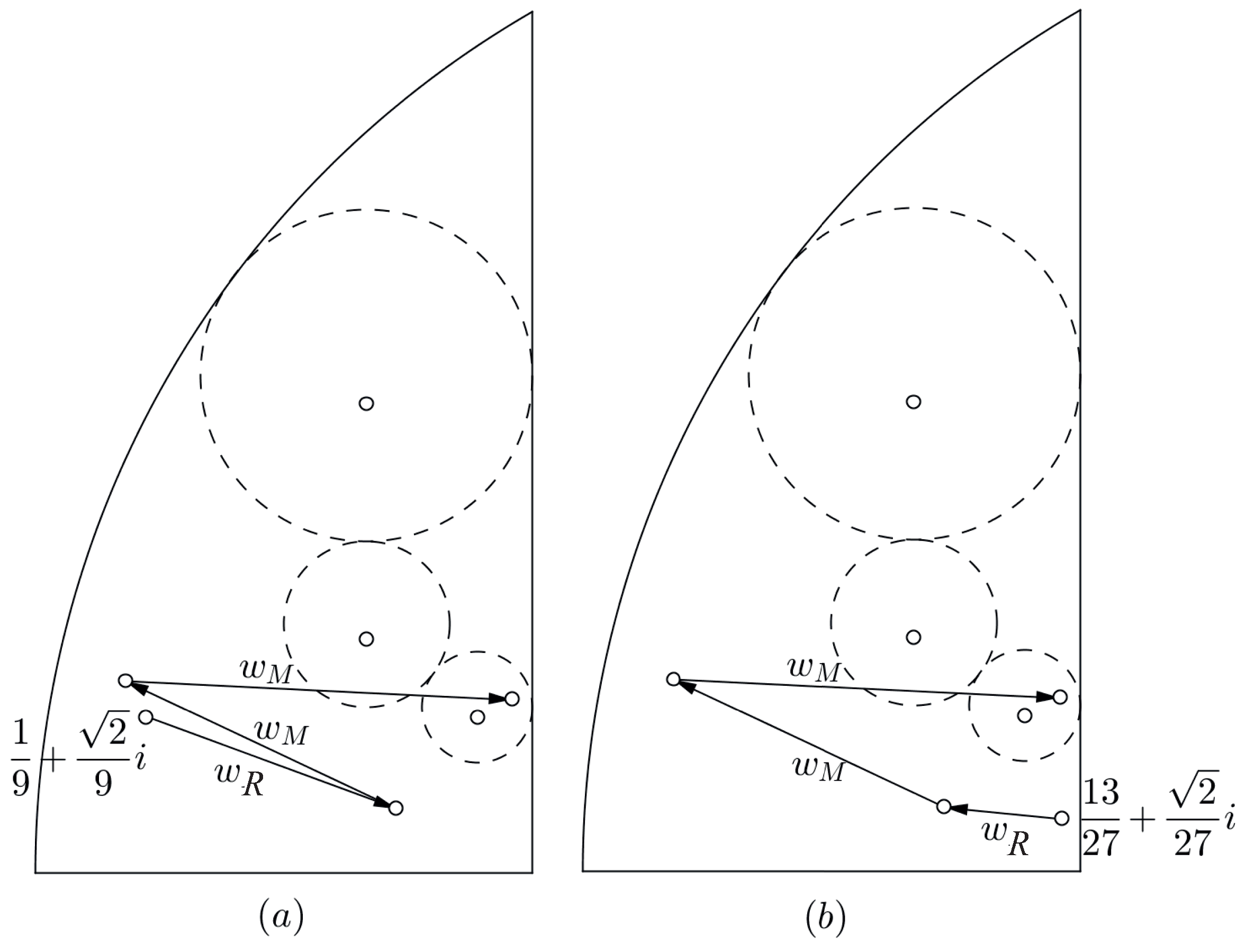
On the other hand, if $W_M^{N-1}\left(z\right)={\omega }_3$, then its pre-image $W_M^{N-2}\left(z\right)$ by $W_M$ is either $\frac{1}{9}+\frac{\sqrt{2}}{9}i$ or $\frac{13}{27}+\frac{\sqrt{2}}{27}i$. Again, it is not possible that $\Gamma \left(z\right)$ is finite, because applying in both cases $W_M^2\circ W_R$ a point is obtained to a distance less than $\ln \sqrt{2}$ to ${\omega }_3$, and again, Proposition 6 applies. See Figure 13a,b. □

5. Conclusions

In this paper, the similarity classes obtained by iterative application of the 3T-LE to an initial triangle have been studied. It has been proved that the number of similarity classes appearing by the iterative application of the 3T-LE to a single initial triangle is not finite in general. There are only three exceptions to this fact: the right triangle with its sides in the ratio 1:$\sqrt{2}$:$\sqrt{3}$ and the other two triangles in its orbit. This result, although of a combinatorial nature, has been proved with the machinery of discrete dynamics in a triangle shape space with the hyperbolic metric defined by the Poincare model in the upper semi-plane. It is also shown that for a point with an infinite orbit, the infinite points of the orbit are in three circles with centers at the points with finite orbits. Similar approaches using this discrete dynamics may be of interest to other triangle transformations. The extension to tetrahedral partitions of a similar approach, to our knowledge, is an open question.