Abstract
In recent years, due to the growing complexity of real-world problems, researchers have been favoring stochastic search algorithms as their preferred method for problem solving. The slime mould algorithm is a high-performance, stochastic search algorithm inspired by the foraging behavior of slime moulds. However, it faces challenges such as low population diversity, high randomness, and susceptibility to falling into local optima. Therefore, this paper presents an enhanced slime mould algorithm that combines multiple strategies, called the ESMA. The incorporation of selective average position and Lévy flights with jumps in the global exploration phase improves the flexibility of the search approach. A dynamic lens learning approach is employed to adjust the position of the optimal slime mould individual, guiding the entire population to move towards the correct position within the given search space. In the updating method, an improved crisscross strategy is adopted to reorganize the slime mould individuals, which makes the search method of the slime mould population more refined. Finally, the performance of the ESMA is evaluated using 40 well-known benchmark functions, including those from CEC2017 and CEC2013 test suites. It is also recognized by Friedman’s test as statistically significant. The analysis of the results on two real-world engineering problems demonstrates that the ESMA presents a substantial advantage in terms of search capability.
Keywords:
enhanced slime mould algorithm; global exploration; lens learning; vertical and horizontal crossover; engineering problem optimization MSC:
68W50
1. Introduction
With the advancement of human society, problems occur, such as in medical image segmentation [1], parameter identification of photovoltaic cells and modules [2], and DNA sequence design [3]. Optimization is a frequently discussed topic in the expanding field of scientific and engineering applications. Generally, optimization is a process aimed at finding the optimal value of a function in various types of problems, which can be continuous or discrete, constrained or unconstrained, at minimum costs. However, most of the optimization problems are nonlinear, high-dimensional, multimodal, and not differentiable [4,5].
Traditional optimization algorithms, such as the gradient descent method, can effectively solve problems involving unimodal continuous functions. The gradient descent method utilizes the gradient information of the function to iteratively update the values of the independent variables, gradually approaching the minimum value of the objective function [6]. The diagonal quasi-newton updating method is based on the concept of the mimetic newton method. It approximates the inverse matrix of the Hessian matrix of the objective function and approximates the diagonal elements of this inverse matrix using a diagonal matrix [7]. The least squares method is used to determine the parameters of the fitted curve by minimizing the squared difference between the observed and fitted values [8], among other things. However, the traditional mathematical methods mentioned above have significant limitations when dealing with complex optimization problems. Firstly, they are unable to handle non-deterministic parameters. Secondly, they are constrained by the feasible domain, which often leads to issues such as insufficient solution accuracy and low solution efficiency. The stochastic search algorithm is a branch of mathematical algorithms that effectively solves the aforementioned problems by utilizing matrix computations involving multidimensional and diverse groups, and by employing random distributions, such as the normal distribution [9], uniform distribution [10], and other distributions from probability theory. This algorithm is advantageous for its gradient-free nature and high adaptability.
SSAs typically involve two phases in their search process: global diversification (exploration) and local precise exploitation (exploitation) [11,12]. In order to adapt to different practical engineering problems, a large number of SSAs continue to appear between the balance of exploration and exploitation, such as monarch butterfly optimization (MBO) [13], thermal exchange optimization (TEO) [14], whale optimization algorithm (WOA) [15], seagull optimization algorithm (SOA) [16], pigeon-inspired optimization (PIO) [17], Harris hawks optimization (HHO) [18], etc.
Although much evidence shows that SSAs are effective optimization methods, when dealing with extremely complex problems, these SSAs can also suffer from phenomena such as premature convergence and being easily trapped in local optima. To improve the trajectory of the stochastic search algorithm’s own population in the search space, researchers have used methods such as chaos maps [19], matching games [20], or a combination of other stochastic search algorithms [21].
Scholars Li et al. [22] proposed a novel stochastic search algorithm—the slime mould algorithm (SMA)—which simulates the oscillations of slime moulds. The SMA utilizes weight changes to replicate the positive and negative feedback processes that occur during slime mould ontogeny in the foraging process, resulting in the emergence of three distinct stages of foraging morphology.
Motivation and Contribution
The SMA has the advantages of simple principles, few adjustment parameters, and high scalability. Although the excellent performance of the SMA has been strongly confirmed, the SMA also has its limitations, such as its high reliance on a single search individual within the group, the absence of a strong global search capability, and the tendency to be trapped in local optimization when dealing with complex high-dimensional problems [23].
It should be noted that the “No Free Lunch” theorem (NFL) [24] implies that any performance improvement of an algorithm in one class of problems may be offset by another class of problems. Although the SMA algorithm has been improved by many scholars, there is still room to further enhance its optimization accuracy. Therefore, it is relevant to propose an improved algorithm with better optimization performance which still has practical significance.
A single search strategy can potentially limit the optimization capabilities of the stochastic search algorithm itself. When a search method has a strong local search capability, its global search capability would be weak, and vice versa. In the SMA, a single search strategy can lead to a lack of population diversity, making it prone to local minima in the solution of complex optimization problems. This suggests that a multi-strategy algorithm has potential.
In this paper, a new search mechanism is proposed to address the inadequacy of the global exploration capability of the SMA. Selective population-averaged positions are used instead of random positions, and a Lévy flight function with jumping characteristics is used to improve the weights of positive and negative feedback. Then, a learning method based on the dynamic lens learning strategy is proposed for fine-tuning the positions of the best individual. Lastly, a practical update method is proposed which utilizes an improved crisscross technique to reorganize the current individuals, generating a perturbation effect on the SMA population.
Among the 40 functions in the test suite of CEC2017 and CEC2014, the ESMA is compared with the AGSMA [25], AOSMA [26], MSMA [27], DE [28], particle swarm optimization (PSO) [29], grey wolf optimizer (GWO) [30], salp swarm algorithm (SSA) [31], HHO, crowd search algorithm (CSA) [32], and SMA. Additionally, a Friedman’s test was conducted for statistical analysis. The results presented above demonstrate the feasibility of the ESMA. The ESMA’s usefulness in solving real-world problems is illustrated through its application to two specific problems: optimizing path finding and designing pressure vessels. The contribution of this paper is briefly described as follows:
- To solve the aimless random search of slime mould individuals and to improve the global exploration capability of the algorithm, a novel approach involving population-averaged position and Lévy flight with conditional selection is proposed.
- To improve the leadership abilities of the best slime mould individual, a novel technique called dynamic lens mapping learning is proposed.
- A novel and improved crisscross method is proposed. This method effectively utilizes the valuable information in dimension of the population renewal process, eliminating the influence of local extremes and consequently enhancing the quality of each solution.
- A total of 40 benchmark functions from the CEC2017 and CEC2013 test suites were employed to evaluate the numerical performance, along with 2 real-world problems to assess the feasibility of optimization. A comparison of the test results between the EMSA and other participating algorithms clearly demonstrates that the EMSA exhibits significantly superior optimization performance.
The remaining structure of this paper is organized as follows: Section 2 provides an introduction to the standard SMA and its related work. Section 3 explains the improved EISMA and its enhancement strategies in detail. In Section 4, the test results on CEC2013 and CEC2017 test suites, as well as the analysis of engineering optimization problems, are presented. Finally, Section 5 discusses the conclusions and future development directions.
2. Background
2.1. Slime Mould Algorithm (SMA)
The SMA simulates the behavioral and morphological changes of slime moulds during the foraging phase, where they search for and surround food. The front of the slime mould exhibits a fan-shaped morphology, which is subsequently accompanied by a network of interconnecting veins. As the veins approach the food source, the slime mould’s bio-oscillator produces diffusive waves, which modify the cytoplasmic flow within the veins. This leads to the movement of the slime mould towards the more favorable food source.
Two crucial parameters for maintaining balance in the SMA are the constant, , and the transition probabilities, . If the number of randomly generated values is less than , the algorithm enters the normal distribution random search stage. If the number of random values, , is greater than or less than , it indicates that the population’s basic search direction has been determined, leading to either the exploration or the development phase. The above shows that the mathematical model of the SMA comprises the following three parts.
2.1.1. Approach Food
When the concentration of food in the air is higher, the oscillator amplitude of the slime moulds becomes stronger, the width of their veins increases, and a larger quantity of slime mould accumulates in the region. Conversely, when the concentration of food in the area is low, the slime moulds will change direction and explore alternative areas. The mathematical model for the movement of slime moulds approaching food is represented by Equation (1):
where, is the current iteration number, is the best individual position, and are the positions of two randomly selected individuals, is the weight coefficient calculated from the fitness, and are the control parameters, respectively, where , linearly decreases from 1 to 0, is a random number between 0 and 1, the search stage is determined by the adaptive transformation variable , and is described as shown in Equations (2) and (3):
where, , is the current individual fitness, is the current best fitness, and is the maximum number of iterations. is the weight coefficient, and it simulates the magnitude of positive and negative feedback produced by the slime mould when encountering different concentrations of food, as shown in Equation (4):
In Equation (4), condition indicates that ranks in the first half of the population, represents a random number following a uniform distribution, represents the best fitness value, is the worst fitness, and represents the sorted fitness indicating the sequence of food concentrations.
2.1.2. Wrap Food
After locating a food source, the slime mould will allocate some individuals to explore other unknown areas randomly, in search of a food source of higher quality. Therefore, the updating of the entire population’s positions is shown in Equations (6)–(8):
where, and are the upper and lower bounds of the dimension of the problem to be solved, respectively, denotes random numbers obeying a uniform distribution, and is a fixed parameter.
Equations (7) and (8) reveal that the SMA alters the search direction of individuals by modifying the parameters , , and . Additionally, it is demonstrated that during the exploration phase, the population moves around the best individual, while during the exploitation phase, the population moves within itself. Furthermore, when the algorithm tends to stagnate, it is also allowed to search in other directions.
2.1.3. Grabble Food
Slime moulds rely on a biological oscillatory response to regulate the flow of cytoplasm in the vein and thus adjust their position to find the optimal food location. To simulate the oscillatory response of slime moulds, the parameters , , and are used in the SMA. represents the behavior of selecting different oscillation patterns based on fitness. It simulates a search pattern where a slime mould chooses its next behavior based on the food situation of individuals at other locations. was utilized to model the process of dynamically adjusting oscillations by changing the diameter of mucus veins based on information from other individuals. is a linear change. It simulates a change in the extent to which the slime mould retains information about its own history.
2.2. Related Work
Currently, many researchers have made a series of improvements to the SMA to make up for the shortcomings of the algorithm itself. They have successfully improved the performance of the SMA at various levels and effectively resolved many real-world engineering problems. The methods for enhancing the performance of the SMA can be broadly categorized into three groups: (1) parameter control, (2) implementation and development of strategies for generating new solutions, and (3) hybridization with other algorithms.
Some important work has been conducted in the literature [33,34,35,36] on the SMA’s control parameters. Miao et al. proposed a novel MSMA in the literature [33]. The algorithm employs a tent map to generate a nonlinear parameter , overcoming the limitation of a constant value. Additionally, it utilizes the randomness of tent map chaos to improve the distribution of elite individuals within the population, resulting in a more reasonable location. The algorithm was applied to a real terraced reservoir system along the Dadu River in China to simulate the maximization of annual power generation. Altay introduced 10 different chaotic maps instead of using the random number to adjust the parameter in the CSMA, as mentioned in the literature [34]. The CSMA evaluates the advantages and disadvantages of the 10 chaotic maps in the SMA algorithm through function testing. Tang et al. in Ref. [35] proposed a new variation called MSMA. It uses two adaptive parameter strategies to improve the SMA parameters, and also employs a chaotic dyadic approach to improve the distribution of the initial population and jumps out of the local optimum with the help of a spiral search strategy. In Ref. [36], Gao noted that the standard SMA employs the arctanh function to compute the parameter a, and subsequently suggested the utilization of the cos function to generate continuous integers for a generation, which is referred to as ISMA.
Several works focused on implementing and developing strategies for generating new solutions, as evidenced by the following literature. Hu et al. [37] were inspired by the ABC algorithm [38] and introduced a variant of the algorithm that incorporates a dispersed foraging strategy named DFSMA. The DFSMA successfully balances global exploration and local exploitation during the iterative process, which has shown promising results on the CEC2017 test suite. Furthermore, it has achieved higher classification accuracy and reduced feature count in feature selection tasks. Allah et al. [39] proposed an improved algorithm called CO-SMA, which is based on the logistic map for a chaotic sequence search strategy (CSS) and incorporates a crossover-opposition strategy (COS) for opposite learning. CSS and COS are transformed by a certain probability . The former is intended to preserve the diversity of solutions, while the latter aims to conduct a neighborhood search around the position of the best individual, thereby enhancing the quality of solution discovery. Results show that CO-SMA minimizes the cost of energy consumption of wind turbines at high altitude. Ren et al. [40] proposed an improved MGSMA by employing two strategies. In this algorithm, strategy 1 applies the MVO strategy with a roulette wheel selection mechanism to the foraging process of slime mould, which partially resolves the issue of getting trapped in local optima. On the other hand, strategy 2 utilizes the Gaussian kernel probability strategy throughout the entire search process. The kernel probability strategy is used during the entire search process, allowing for the perturbation of newly generated solutions and expanding the search range of the slime mould individuals. Furthermore, MGSMA demonstrated improved performance in multi-threshold image segmentation. Ahmadianfar et al. [41] proposed an improved version of MSMA that incorporated three enhancements. Firstly, they introduced additional parameters, such as the number of iterations, into the mutation operator of the differential evolution (DE) used in MSAM. Secondly, they introduced an effective crossover operator with an adjustable parameter to enhance the diversity of the population. Lastly, they utilized a deviation from the current solution to further improve the solution quality. Simulation experiments showed that MSAM significantly improved the generation performance of multi-reservoir hydropower systems. Pawani et al. [42] addressed the issue of insufficient local exploitation in the SMA when dealing with complex searches that involve a wide range of neighborhood optima. To tackle this problem, they proposed a method called WMSMA that utilizes wavelet mutation to adapt individuals and prevent them from getting trapped in local minima. It effectively solves the cogeneration scheduling problem with nonlinear and discontinuous constraints. Sun et al. [43] proposed two strategies to enhance the SMA. The first strategy, called the BTSMA (Brownian motion and tournament selection mechanism SMA), focuses on improving global exploration by incorporating Brownian motion and tournament selection. The second strategy involves integrating an adaptive hill climbing strategy with SMA to promote the development trend, thus facilitating the local search. Experimental results on structural engineering design problems and training multi-layer perceptrons validate the effectiveness of the BTSMA in real-world tasks.
An active research trend is to combine the SMA with other evolutionary computation techniques, as evidenced by the following literature. Zhong et al. [44] proposed a hybrid algorithm (TLSMA) that utilizes a teaching-based learning optimizer (TLBO) integrated with the SMA. The TLSMA is divided into two subgroups with dynamic selection, where the former utilizes a TLBO search and the latter employs an SMA search. This division improves the optimization capability of the SMA. Performance gains are achieved in simulating five RBRO problems, including the problem of optimizing numerical design. Liu et al. [45] proposed a hybrid algorithm called MDE, which utilizes the DE algorithm exclusively. After the mutation, crossover, and selection steps, the SMA begins searching for the optimum in the search space using the improved population. This approach, known as MDE, helps mitigate the risk of falling into a local optimum, to some extent. MDE effectively carries out multi-threshold segmentation of breast cancer images, achieving satisfactory results. Lzcili [46] proposed a refined algorithm, called OBL-SMA-SA, which introduces SA [47]. The algorithm features a mechanism that allows for the acceptance of suboptimal solutions with a probability, p, during global exploration. Additionally, an opposite learning approach is employed for local exploitation. The combination of these two strategies aids in mitigating the risk of getting trapped in a local optimum. OBL-SMA-SA efficiently adjusts the parameters of the FOPID controller, ensures the stability of the automatic voltage regulator’s endpoint voltages, and regulates the speed of the DC motor. Örnek et al. [48] were inspired by the SCA [49] and introduced a variant of the SMA, called the SCSMA. The SCSMA improves the algorithm update process by leveraging the reciprocal oscillation property of sine and cosine during each iteration, which effectively advances the algorithm’s exploration and development. The efficacy of SCSMA is validated through its application to real-world problems, including the design of four cantilever beams. Yin et al. [50] proposed an improved algorithm called EOSMA. During the exploration and development phase, EOSMA exchanges the roles of the best individual and the current individual. Then, the random search phase of the SMA is replaced by the EO [51]. Finally, it is supplemented with a different Mutation strategy to increase the probability of escaping from local optima. The superior optimization capability of EOSMA is demonstrated through its application to nine problems, including the design of a car in a side-impact collision.
In summary the SMA variant algorithms and their applications are shown in Table 1.

Table 1.
Summary of algorithms.
Figure 1 shows the steps of the whole search process of the SMA.

Figure 1.
Search process of the SMA.
The pseudo-code of the SMA is as follows in Algorithm 1.
| Algorithm 1 SMA |
| 1. Input: the parameters N, , the positions of slime mould ; |
| 2. |
| 3. while ( do |
| 4. Calculate the fitness of all slime mould; |
| 5. Update best fitness and best position ; |
| 6. Calculate the by Equation (4); |
| 7. for |
| 8. Update ; |
| 9. if |
| 10. Update positions by Equation (6); |
| 11 else if |
| 12. Update positions by Equation (7); |
| 13 else |
| 14. Update positions by Equation (8); |
| 15 end if |
| 16. end for |
| 17. ; |
| 18. end while |
| 19. output: ; |
3. Enhanced Slime Mould Algorithm That Combines Multiple Strategies (ESMA)
In order to improve the optimization search capability of the SMA, three different approaches are proposed to address each of its three deficiencies: (1) An effective global search method can be achieved by utilizing a conditional mean position of the population along with a Lévy function that incorporates a non-deterministic random walk mechanism. (2) Efficiently learning the best individual can be accomplished through the implementation of a dynamic lens-based learning method. (3) By employing an enhanced method of updating slime mould individuals using dimensional crossover, the updating process can be improved to prevent falling into local optima.
3.1. A New Global Search Mechanism
In SSAs, search techniques demonstrate superior performance when they exhibit strong exploration ability during the initial and intermediate stages of the global search. For instance, in Tang’s study [52], the tabu search technique based on the critical path and critical path method was employed to augment the number of teachers in the dynamic teacher group during the global exploration stage of the process.
There are two important features in the early global exploration process of the SMA. (1) When , the step-size portion of the slime mould’s position update is computed by combining the positions of two random individuals using and . During this stage, the search behavior of the slime mould is characterized by aimless and random exploration [25], which partially undermines the effectiveness of the preliminary search of the SMA. As a result, a rational selection of search individuals becomes crucial. (2) The appropriate magnitude of the weighting factor , used to simulate the positive or negative feedback between the pulse width of the slime mould and the concentration of explored food, restricts the extent of perturbation in the current random individual, thereby influencing the global exploration capability of the algorithm. To solve the aforementioned challenges, the following discussion is conducted.
Fusion of other populations individual positions iteratively superimposed inertia weights and other parameters to compose the global exploration of the updating method.
Facilitating the exchange of information regarding the positions of individuals in the current population is a beneficial search strategy in stochastic search algorithms. Inspired by the AO algorithm [12] that utilizes the average position of the population for global exploration. However, the average position of the population does not always play a dominant role in the search. Therefore, in this paper, random individuals with the weighting factor are replaced in this paper with a conditionally selective population average position in the exploration Formula (7) of the SMA. This approach allows for the better sharing of information and positions with other individuals, as well as the advantage of learning from the information obtained from other individuals in the population. The average population position is shown in Equation (9).
where, in Equation (9), is the population size and and are the location and dimension component of the current individual, respectively.
Next, the question of the proper use of the location is discussed in detail. In other words, how to use the position conditionally. Case (1): Typically, individuals in proximity to the best individual tend to have a shorter Euclidean distance compared to other individuals. The in Equation (10) reflects the distance between the average individual of the population, a random individual , and the leader slime mould . Case (2): Based on the aforementioned distance conditions, if the randomly selected slime mould in the search space deviates from the direction leading to the global best position, updating its position with the location of an individual that has a better fitness value can enhance its search ability. Equation (11) reflects the relative fitness of the average position and .
where is the random position, is the average position, is the best position, and is the problem function to be solved.
Furthermore, determining how to improve the weighting factor, , becomes crucial for solving the global exploration problem. The compliance with uniformly distributed random numbers, , in SSAs lack a jumping mechanism. Author Altay, in Ref. [31], has demonstrated in detail how the introduction of a suitable method can effectively upgrade the weighting factor,.
It is well known that Lévy flight is a specific random variable that follows a random walk that follows a non-Gaussian distributed random walk to solve the stagnation problem in SSAs. It moves in both small range wandering and large distance jumping [53,54]. In this paper, in order to improve the rational feedback of the weight factor on the search of slime mould individual, expand the leap capability of the algorithm, and also prevent the algorithm from falling into a local optimum. Lévy variables are generated according to Equation (12). The Lévy random variable is then incorporated into the weighting factor, W, as depicted in Equation (14). Lévy variables are generated as shown in Equation (12).
where is a fixed value of 0.01 and and are random numbers between 0 and 1, respectively. The value of is calculated using Equation (7).
where is set to a fixed value of 1.5.
where is the value of the Lévy function produced by Equation (12).
To address both of the aforementioned problems, a proposed global exploration update method is presented in Equation (15). This method combines the average position of the population with the Lévy function as an improvement strategy.
3.2. An Effective Learning Method
During the search process of the standard SMA, the leader slime mould guides the population to conduct an extensive search within the specified problem boundaries. This optimization process can be considered as employing an elite strategy, where the search method directly influences the overall search performance. Therefore, it is crucial for the leader slime mould individual to possess a flexible search mechanism. Furthermore, the update operation of the leader individual in the SMA is exclusively determined by the fitness evaluation. According to Equation (7), as the number of iterations increases, the entire population of slime moulds will gradually converge towards the current best position. This convergence tendency poses a challenge for the SMA, as it increases the likelihood of getting trapped in local optima when attempting to solve complex multi-model functions.
The algorithm’s susceptibility to falling into local optima has been extensively studied. It has been observed that the opposite solution of the majority of population individuals is often closer to the best point than the inverse solution of ordinary population individuals. This suggests that it is easier to escape local optima. This finding is supported by multiple studies [55,56]. Equation (16) represents the standard opposition learning form, which solves the optimization problem in one fixed direction. However, it still carries the risk of monotonicity and local optimization in other search directions.
where, and are the upper and lower boundaries of the given problem, respectively.
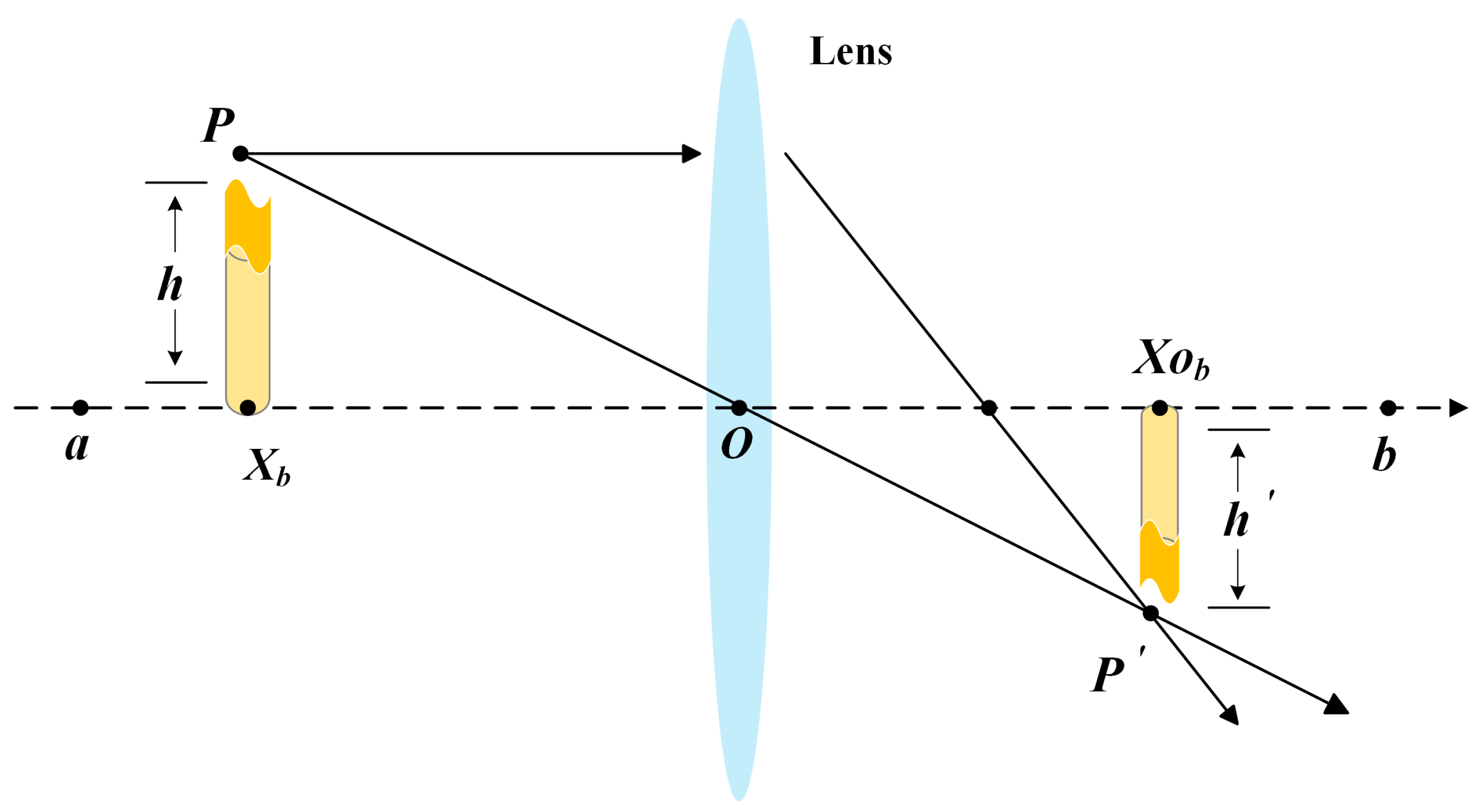
Lens learning, based on opposition learning [57], increases the search in various directions within the search space. As a result, the generated opposition individuals exhibit flexible diversity, which is advantageous for exploring unknown domains. The principle of opposition learning is illustrated in Figure 2. In this context, the principle of standard lens learning is assumed to operate within a given two-dimensional plane. The height of point is represented as, and represents the projection of point onto the transverse coordinate axis. The center of the lens is set at point , where . By performing the imaging operation, the height, , of point on the transverse coordinate axis can be obtained, with its projection denoted as . Based on the above, a new point, , can be generated through the imaging operation, as expressed mathematically in Equation (17).
where, let , the transformation of Equation (17) is adjusted as shown in Equation (18).
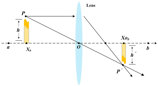
Figure 2.
Lens imaging principle.
From the transformed Equation (18), it can be observed that the size and direction of the new point, , are determined by the parameter . The newly generated solutions, based on the lens learning principle, are converted into the perturbation and updating of individual population members in the stochastic search algorithm, while the dynamically scaled parameter, , helps improve the randomness of the generated population members.
The principle of lens learning in the two-dimensional plane, described above, is used to avoid biased search individuals resulting from unreasonable upper and lower bounds in the lens learning process. In general, better results can be achieved by using the upper and lower bounds of the decision variables of the current iteration individuals in SSAs. To enhance the leadership ability of the best slime mould individual in the ESMA, a new lens learning strategy is proposed based on the aforementioned principle, which adjusts the current position in the problem area being solved. However, the dimensions of complex functions vary. To accommodate the high-dimensional position vector of the leader slime mould individual in the ESMA, it needs to be generalized to a multidimensional state, as shown in Equation (19).
where and are the maximum and minimum components of , respectively, and is the dimensional component of the best individual after lens learning.
Equation (19) produces the best position of the individual after performing multidimensional mapping. Parameter , which controls the direction and distance of the search, affects the angles and distances between the original best individual and the newly generated best individual. It also enhances the ability of the best individual to move in the best direction within the search space. To improve the applicability of the lens learning method to the ESMA, the parameters are adjusted and a dynamic parameter, k, based on the number of iterations, is proposed. The dynamic parameter, , is given by Equation (20).
In Equation (20), is 0.5 and is 10 after several experiments.
Finally, the next iteration is updated by selecting the best individual between at the current iteration and the formed by lens learning, as shown in Equation (21).
3.3. A Feasible Update Method
As a population-based stochastic search algorithm, the search process of the SMA can be primarily categorized into two phases: global exploration, where the objective is to approach food, and local exploitation, where the focus is on wrapping food. However, during the exploration stage of the SMA, two random individuals with position vectors are utilized to search around the best individual. On the other hand, during the local exploitation phase, the update method is computed solely based on the current individual and the Oscillatory factor for linear descent oscillations . As the depth of population iteration increases, the concentration degree of individuals greatly improves. However, this also leads to an increase in the probability of stagnation during the iterative process, resulting in a significant reduction in population diversity. In other words, the solutions obtained by the SMA in each search may not always be reliable. The jump-out mechanism makes it susceptible to encountering local extremes, leading to the occurrence of premature states. This weakness in seeking the best solution to the problem can be addressed by combining the SMA with other stochastic search algorithms [58,59].
The crisscross optimization algorithm (CSO) [60] is a stochastic search algorithm that alternates with a unique double crossover operator. The dimensions of the search individuals are combined and crossed in two different ways, horizontally and vertically. This approach aims to fully utilize the useful information from each dimension in solving the objective function, thereby mitigating the influence of local extremes and enhancing the quality of the solution. In this paper, we leverage the unique capability of CSO to capture dimensional information and propose an improved CSO search strategy that incorporates the ESMA to refine the fusion of information among individuals.
3.3.1. Horizontal Crossover
The horizontal operator in the CSO conducts the crossover operation within the same dimension of two individuals from the population in a randomized and non-repetitive manner, as shown in Equations (22) and (23).
where and are random numbers between 0 and 1; and are random numbers selected from the interval [−1, 1], respectively; and and represent the jth dimensional positions generated by slime shapes and , respectively, after crosswise crossover. The dimension for vertical crossover is selected as the better one between the two. is the subscript of the random individual.
The influence of random numbers and are chosen from the interval [−1, 1] on the dimensional distance between two random individuals and in a standard CSO. To some extent, this operation will lead to the emergence of an unordered stochastic state during the search process. To change this phenomenon, the sine and cosine functions are utilized instead of the random numbers and to regulate the distance control, as shown in Equations (24) and (25).
The combination of sine and cosine functions in the algorithmic search process exhibits the characteristic of seeking constant oscillations between each other within a given space. This feature enables the algorithm to consistently maintain the population’s diversity among the individuals involved in the horizontal crossover phase. Figure 3 presents a schematic diagram illustrating the operational process for function values within the range of [−1, 1]. Through the horizontal crossover operation, diverse individuals are able to exchange information, facilitating an enhanced global search capability as they learn from each other.
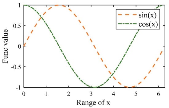
Figure 3.
Crossover of sine and cosine functions.
3.3.2. Vertical Crossover
In the later stages, the SMA is susceptible to becoming trapped in local optima. This phenomenon primarily occurs when some individuals within the population succumb to local optima in a particular dimension, consequently causing premature convergence of the entire population. The SMA itself lacks the capability to regulate individuals that have become trapped in local optima, impeding the search process and limiting the potential for discovering the global best solution. Therefore, the advantageous solutions resulting from horizontal crossover are selected as parent populations and subjected to Vertical crossover, which operates between two different dimensions within an individual.
Assuming that the newborn individual, denoted as , corresponds to the individual with subscript , in the dimension, and undergoes longitudinal crossover in the dimension. The calculation is depicted in Equation (26).
where is the offspring individual generated from the and dimensions of individual by vertical crossover, and .
The competitive mechanism, as shown in Equation (27), incorporates slime mould individuals engaged in crossover, thus minimizing the risk of losing important dimensional information. This mechanism effectively enhances population diversity and consistently improves solution quality. The individuals who have fallen into the local optimum can make full use of the information in each dimension, and thus have the opportunity to jump out of the local optimum.
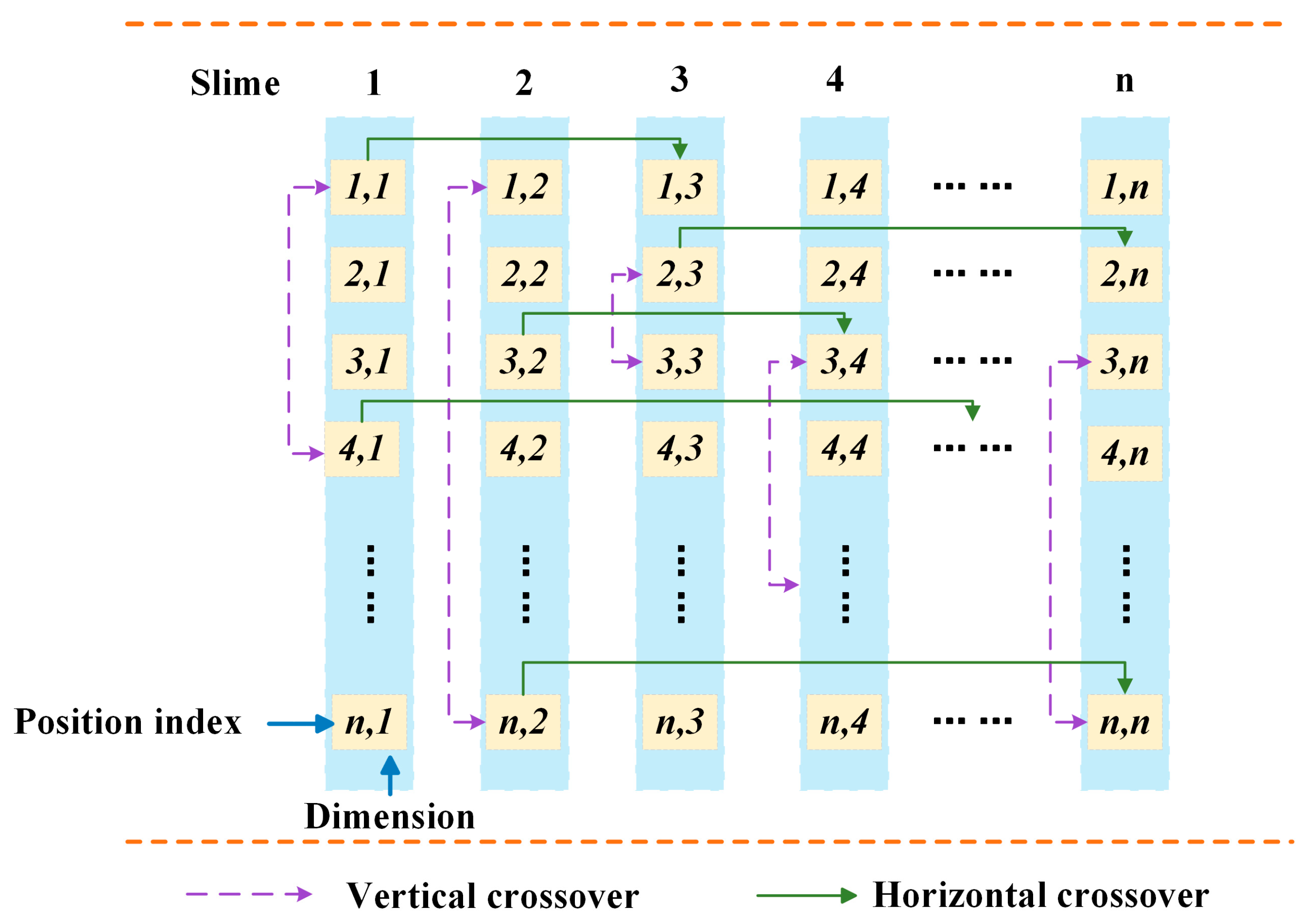
In summary, after horizontal crossover between slime moulds, individuals with oscillatory properties in the preliminary to intermediate stages phases, and vertical crossover within individuals in the later phases, the degree of aggregation of the population was greatly reduced and the diversity of the population was increased. Figure 4 shows the process of horizontal and vertical crossover.

Figure 4.
Process of horizontal and vertical crossover.
3.4. Improved ESMA
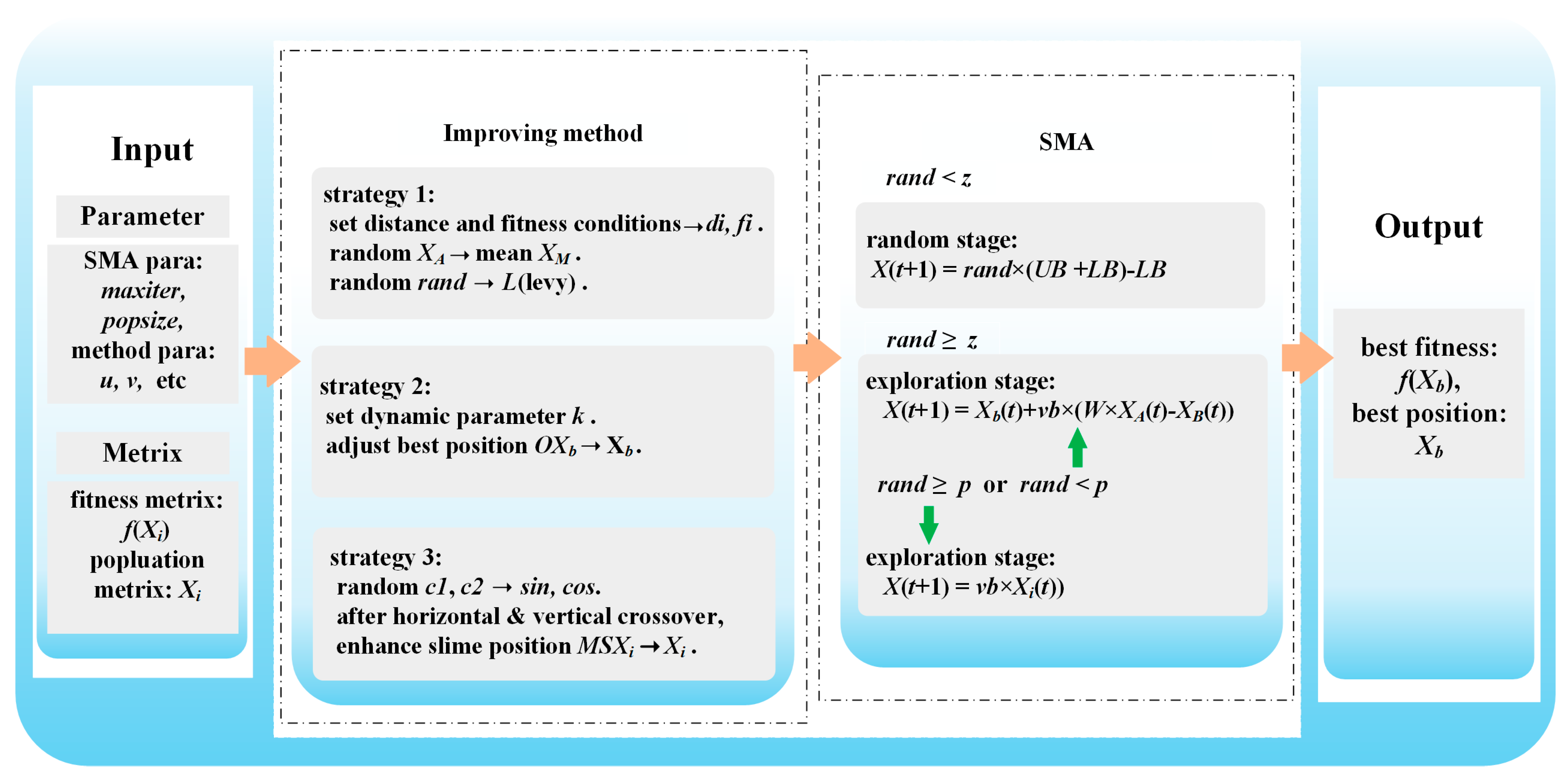
The aforementioned improvement approaches are synthesized, followed by a concise description of the enhanced slime mould algorithm (ESMA) proposed in this paper. The ESMA first uses a new search mechanism that incorporates a global search method modified by a strategy of population mean position and Lévy flight function to the algorithm’s ability to explore unknown space in the pre-intermediate period. Then, a new learning method is proposed, which adopts the dynamic parameters to adjust the search angle and distance of lens learning to generate better leader slime mould individuals to achieve the goal of better guiding the whole population. Finally, a feasible update method is proposed. The method adopts the vertical and horizontal and cross-sectional approaches to reorganize the dimensions of the slime mould individuals, thus the SMA adds a perturbation mechanism, which is of great benefit to improve the algorithm’s ability to find the best solution.
Figure 5 shows the algorithmic workflow of the ESMA, which incorporates three improvement strategies.
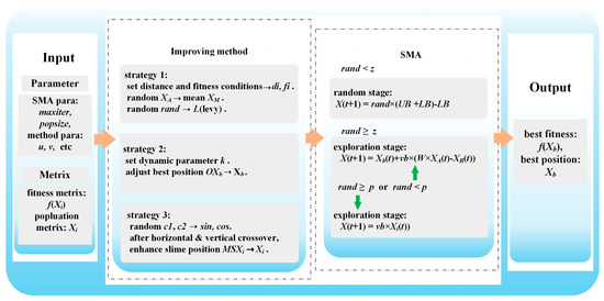
Figure 5.
Scheme of the ESMA.
The pseudo-code of the ESMA is as follows in Algorithm 2.
| Algorithm 2 ESMA |
| 1. Input: the parameters N, , the positions of slime mould ; |
| 2. |
| 3. while |
| 4. Calculate the fitness of all slime mould; |
| 5. Update best fitness and best position ; |
| 6. Calculate the by Equation (14); |
| 7. Calculate the , by Equations (10) and (11); |
| 8. for |
| 9. Update ; |
| 10. if |
| 11. Update positions by Equation (6); |
| 12. else if |
| 13. Update positions by Equation (15); |
| 14. else |
| 15. Update positions by Equation (8); |
| 16. end if |
| 17. end for |
| 18. for |
| 19. Calculate horizontal crossover positions by Equations (24) and (25); |
| 20. Calculate vertical crossover positions by Equation (26); |
| 21. end for |
| 22. Calculate Lens learning position by Equation (19); |
| 23. Update best position by Equation (21); |
| 24. ; |
| 25. end while |
| 26. output: ; |
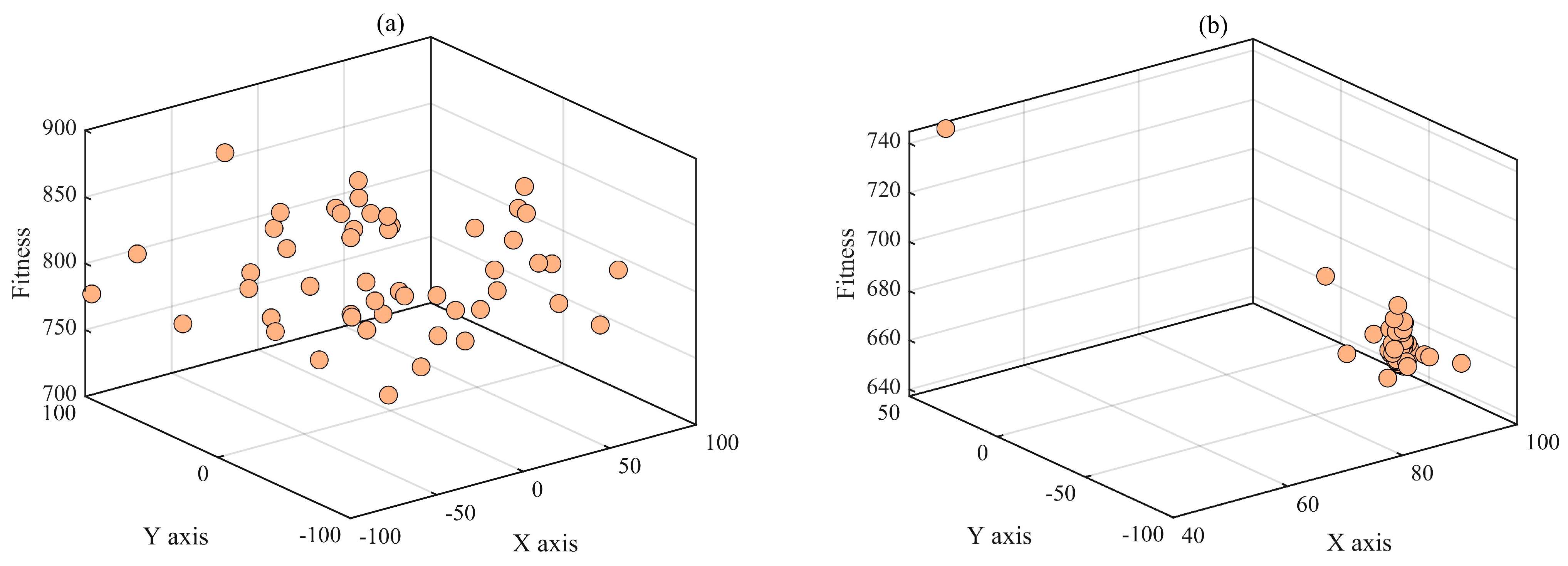
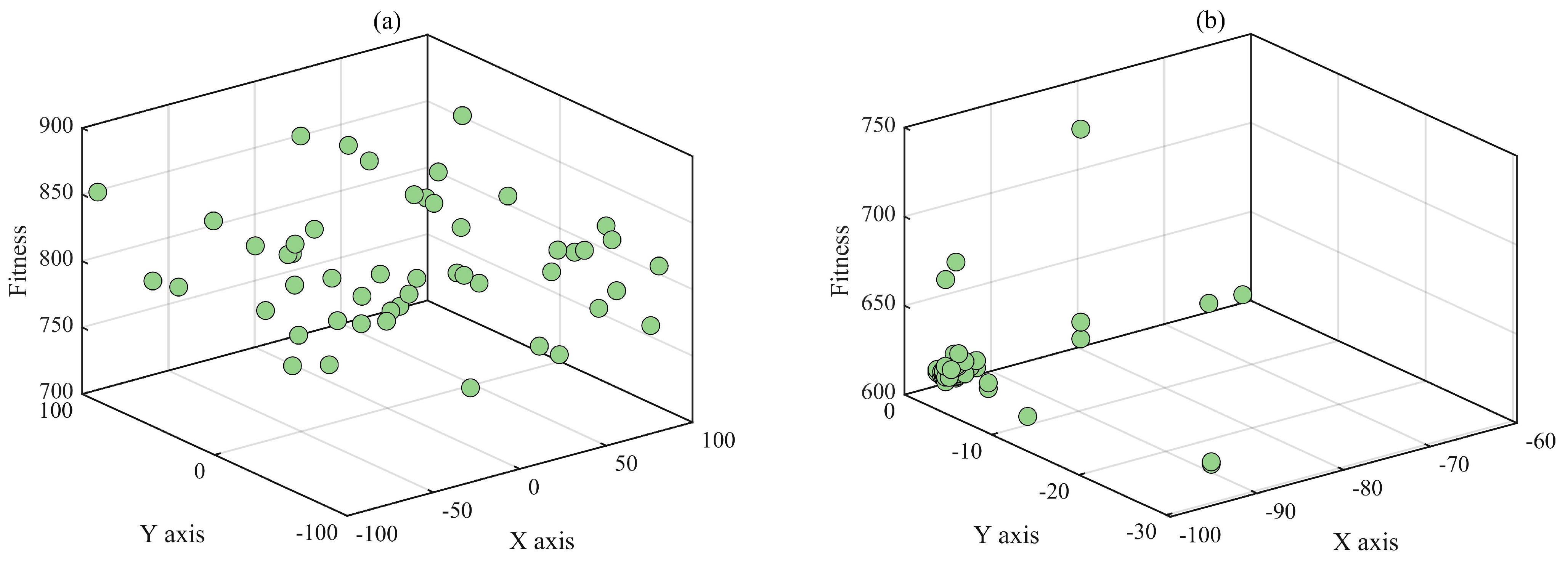
To demonstrate the improved optimization mechanism of the ESMA and validate its scientific rigor and effectiveness, this paper adopts the CEC2017 Multimodal Function Shifted and Rotated Expanded Scaffer’s F6 Function as the test benchmark. Additionally, two algorithms are employed in the optimization process to analyze the individual distribution graph. Assuming that the maximum number of iterations is 200 and the number of populations is 50, the individual distribution plots of the two algorithms are shown in Figure 6 and Figure 7. The ESMA rapid convergence can be seen, as evident from the more dispersed distribution of individuals from initial to final stages. This improved population diversity is attributed to most individuals closely following the leader individual, which approach the best value. Conversely, the SMA exhibits slow convergence and remains trapped in local optimal points, as indicated by its concentrated state.
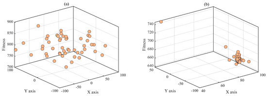
Figure 6.
Individual distribution of the SMA. (a) The SMA individual initialization map. (b) Individual distribution of the SMA in 100 generations.

Figure 7.
Individual distribution of the ESMA. (a) The ESMA individual initialization map. (b) Individual distribution of the ESMA in 100 generations.
3.5. Complexity Analysis
This paper employs the O notation to compute the time complexity. The improved ESMA mainly includes the following parts: random initialization, fitness value evaluation, sorting, position update, and distance judgment. Assuming that the number of slime mould populations is , the dimension of the problem is x, and the maximum number of iterations is , then the computational complexity of initialization is , the computational cost of sorting is , the computational complexity of weights updating is , the time complexity of population position updating is , the computational complexity of distance judging is , the computational complexity of the lens learning method is , the complexity of parameter tuning is , and the complexity of horizontal and vertical crossover is the same as the population position update, which is . In summary, the total complexity of the ESMA can be estimated as follows: .
4. Experimental Results and Discussion
In this section, the performance of the ESMA is verified by 40 standard test functions and 2 real-world optimization problems. The entire testing procedure is structured as follows: (1) establishment of experimental criteria and setup, (2) comparison of results obtained from CEC2017 functions, (3) comparison of results obtained from CEC2013 test functions, (4) execution time, (5) statistical test, (6) analysis of diversity in the ESMA, (7) analysis of exploration and exploitation in the ESMA, and (8) comparison of the results obtained from real-world engineering problems.
4.1. Experimental Criteria and Setup
There are 29 CEC2017 and 11 CEC2013 test functions used in this test. Generally, unimodal functions, which typically have a single global optimum, are commonly employed to evaluate the efficacy of SSAs. Additionally, the aforementioned multimodal functions are more intricate than unimodal functions, exhibiting numerous local optimum solutions. These multimodal functions can be utilized to examine the exploration capability of optimization techniques. Furthermore, composite and hybrid functions encompass a combination of the aforementioned two types of functions.
The parameter selection is mostly based on the parameters used by the original authors in the various literature. Due to the longer development time of PSO and DE, the parameter settings for PS were obtained from reference [19], while parameters for DE were determined based on extensive research conducted by various researchers, as described in reference [61], in order to achieve better performance. Detailed parameter settings are presented in Table 2. Table 3 presents the categorization of function used in the experiment. In CEC2017 test functions, F1–F2 are classified as unimodal functions, F3–F9 as multimodal functions, and F10–F19 as hybrid functions. Moreover, F20–F29 are composition functions. The CEC2013 test functions consist of F30–F31 as unimodal functions, F32–F38 as multimodal functions, and F39–F40 are composition functions. The experiment incorporates a total of 11 comparison algorithms, including three variants of the SMA (AGSMA, AOSMA, and AOSMA), six widely recognized stochastic search algorithms (DE, PSO, CSA, HHO, SSA, and GWO), and the standard SMA with the improved ESMA.

Table 2.
Parameter settings for each algorithm.

Table 3.
Standard test functions.
To ensure consistency and reliability, the aforementioned algorithms were implemented for 1000 iterations, with a population size of 30 individuals, to solve the designated test benchmark problem. Thirty independent tests were conducted, and the mean (Mean), standard deviation (Std), and best solution (Best) of the results are provided. The experiments were carried out on a PC with an Intel Core i5-5800H CPU @ 2.30 GHz and the Windows 10 operating system. MATLAB R2021a software (version number is 9.10.0.1601886)was employed for calculating the test results.
Friedman’s test was utilized to assess the statistical significance of differences by examining the rank of ESMA in the tables below. The Friedman rank, , of the algorithm was calculated using the following procedure:
The statistical distribution, , is shown in Equation (29).
4.2. CEC2017-Based Effectiveness Analysis
This subsection provides a detailed analysis of the test results for each participating algorithm, based on the CEC2017 functions in dimensions of 30 Dim, 50 Dim, and 100 Dim, respectively.
Table 4 presents the experimental data obtained from simulating the ESMA with 11 participating algorithms across 29 functions, each with a dimension of 30. It can be shown that the ESMA has an excellent performance in terms of mean value (Mean) compared to other algorithms. The ESMA achieves the highest rank, with a Friedman Rank of 1.7241, placing first in the overall ranking across 19 functions. These functions include unimodal F1–F2, multimodal F3, F5–F6, hybrid F10–F12, and combined F25–F28. In contrast, the standard SMA, which did not achieve first place in any of the functions, obtains a Friedman Rank of 4.3793, ranking fourth overall. The variant algorithms AGSMA, AOSMA, and MSMA have Friedman Rank values of 2.5172, 3.5172, and 5.0345, respectively. Among the other six stochastic search algorithms, namely DE, GWO, HHO, PSO, CSA, and SSA, only GWO achieved first rank in F16 with Friedman Rank values of 8.6552, 5.7241, 7.8276, 10.0690, 6.5172, and 10.0345, respectively. In terms of the best value “Best”, the ESMA achieved the first-ranked best value in function F19, F20, and four other functions, even though the mean value did not reach the best. This indicates that the ESMA not only exhibits superior performance but also demonstrates better robustness, as evidenced by its lower standard deviation (Std).

Table 4.
Result of the ESMA 30 Dim on CEC2017 functions.
The enhanced global exploration approach, which incorporates mean and Lévy flight functions, dynamic lens mapping learning, and dimensional reorganization of search individuals during iterations, significantly enhances its ability to locate the optimum. As a result, it becomes more effective at solving complex problems by reducing the risk of getting trapped in local optima.
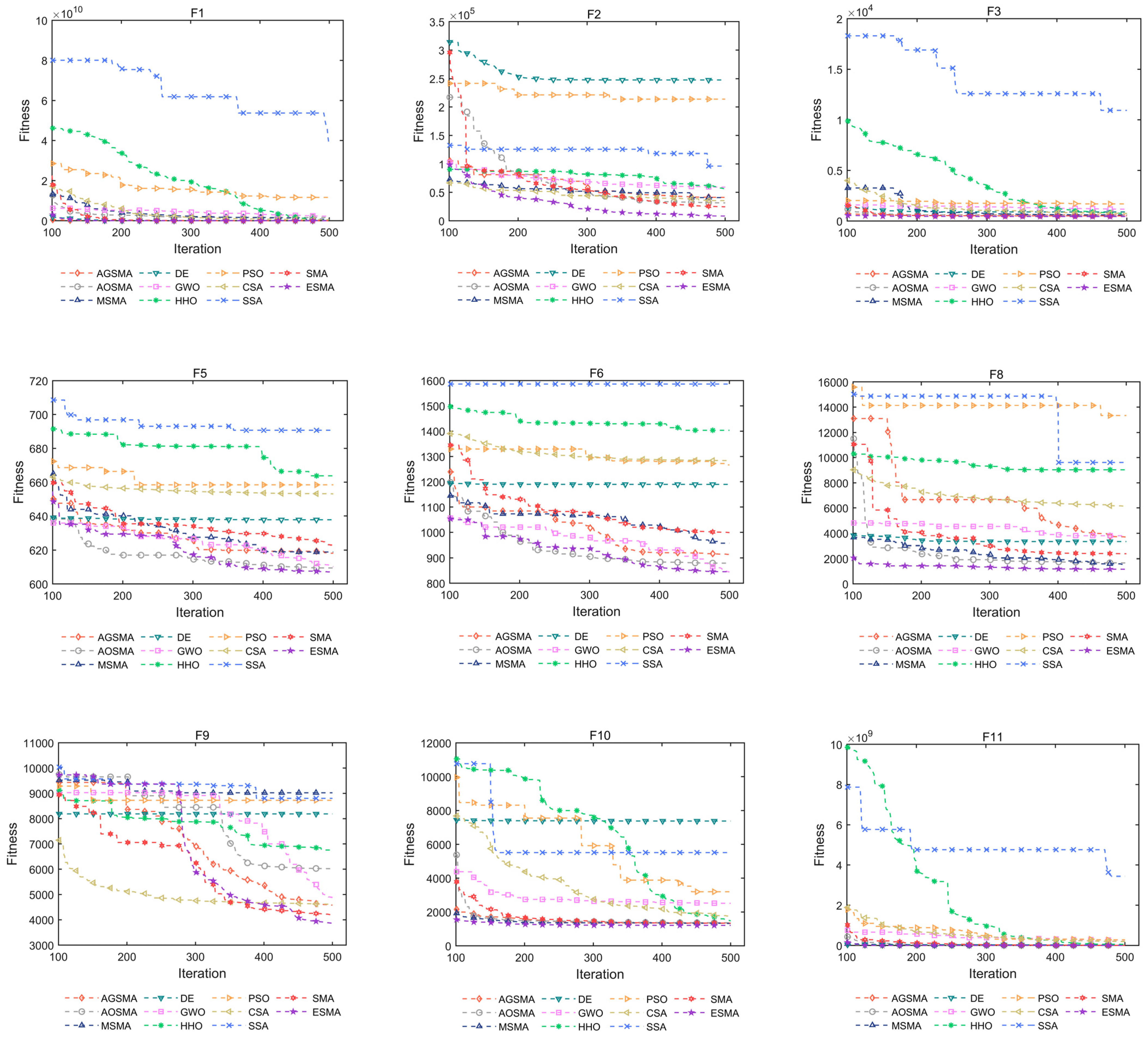
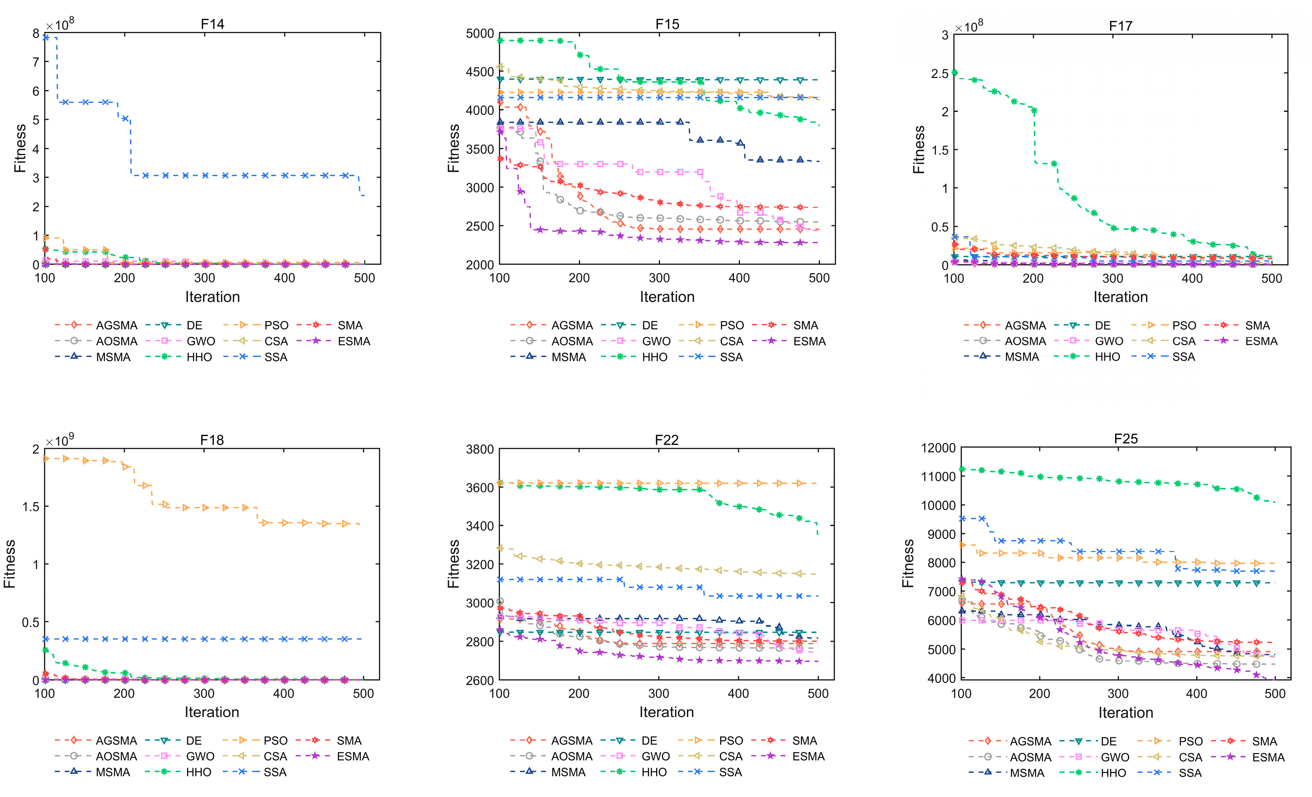
Figure 8 lists the convergence curves of 15 representative functions. The ESMA demonstrates rapid convergence and high solution quality for unimodal functions (F1 and F2). Additionally, the ESMA exhibits significantly superior optimization accuracy for multimodal functions. It is worth noting that for eight complex hybrid and composition functions such as F10, the performance of the ESMA remains unaffected, while the clustering of the convergence curve is due to the fact that the solution values represented by PSO are too large, i.e., the function is trapped in a local optimum. These results demonstrate the effectiveness of the ESMA in searching the unknown space of a given function. Furthermore, the experimental results presented above indicate that employing multiple strategies enhances the SMA by improving population diversity, accelerating convergence speed, and enhancing the ability to search for the best solutions.
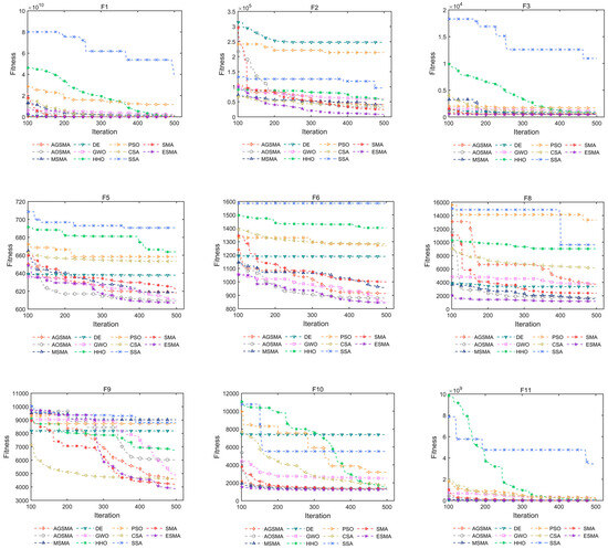
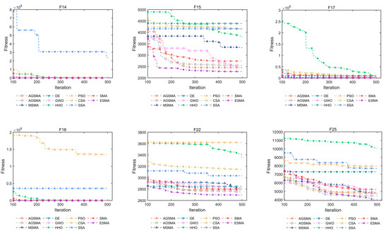
Figure 8.
Convergence curves for each comparison algorithm.
Table 5 shows the effectiveness of the improvement method employed by the ESMA in a 50 Dim environment. The utilization of the three improvement strategies significantly enhances the algorithm’s run speed in high-dimensional spaces, enabling faster contraction of the solution space and laying the groundwork for local development. The ESMA also exhibits greater stability and robustness when compared to the comparison algorithm. The results indicate that the ESMA demonstrates superior performance, consistently achieving the highest ranking in finding the best value for 19 out of 29 functions. With a Friedman average rank of 1.6207, the ESMA accounts for 65.5% of the total, solidifying its dominance in the evaluation. The variant AGSMA achieves the search best value in 13.8% of the functions, while the AOSMA achieves it in 17.2%. On the other hand, the MSMA and SMA do not achieve the best value in any of the functions, with Friedman average ranks of 2.7241, 3.0690, 5.9655, and 3.8276, respectively. In contrast, other stochastic search algorithms such as DE, HHO, PSO, CSA, and SSA do not outperform any function. Only the GWO algorithm secures the first place in one function, specifically F15. The majority of functions falling under multimodal, hybrid, and composition categories, where the ESMA excels, confirms its ability to strike a better balance between exploration and development phases and effectively handle combinatorial functions with multiple local optima.

Table 5.
Result of the ESMA 50 Dim on CEC2017 functions.
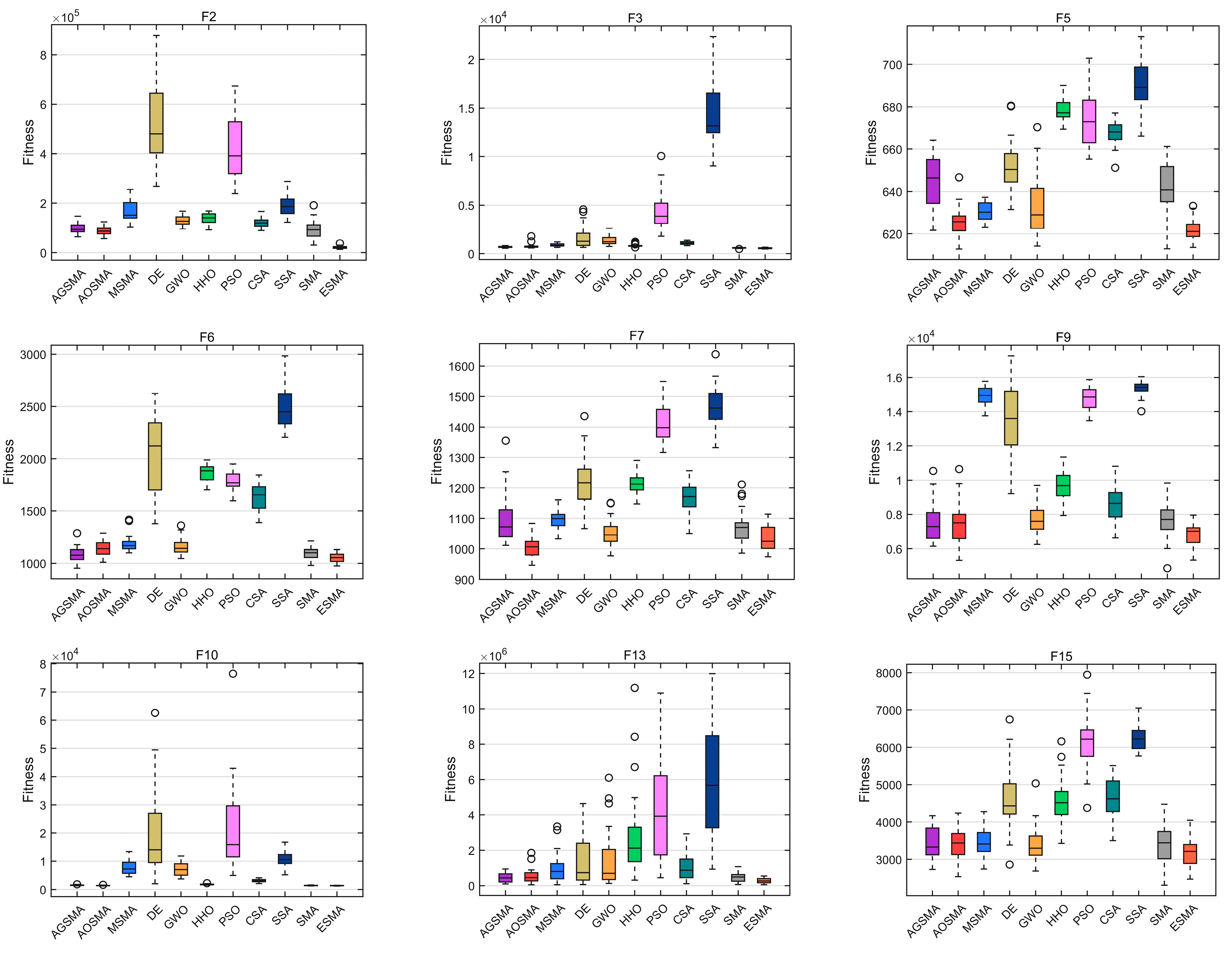
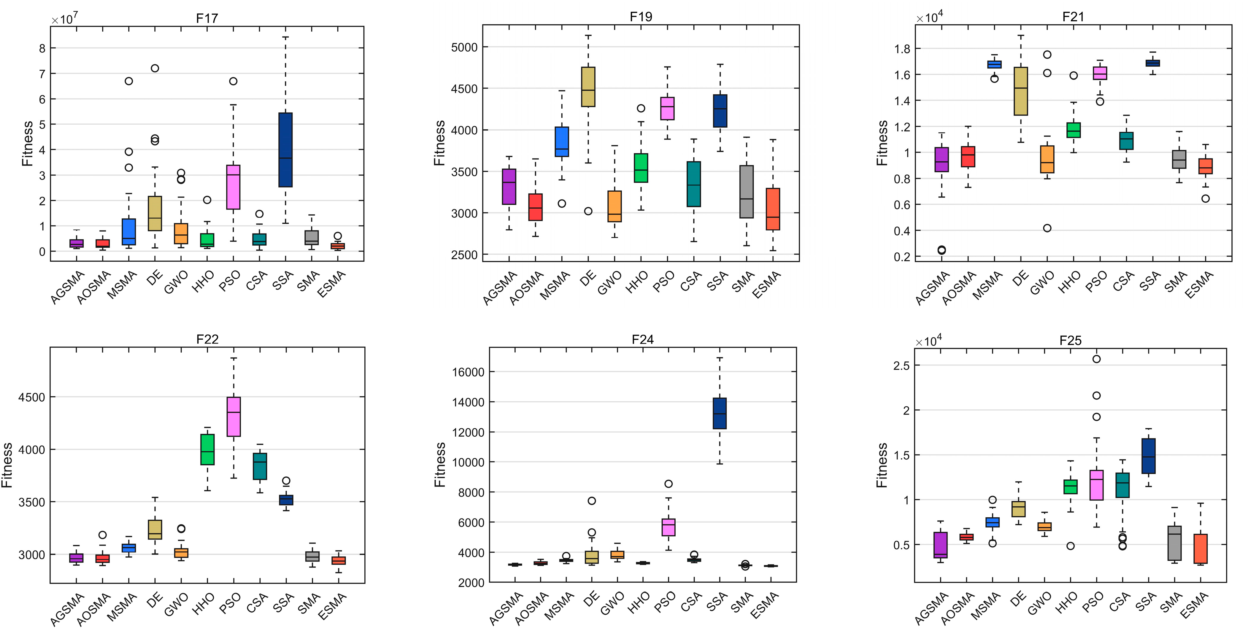
Figure 9 presents the boxplots of the 15 CEC2017 functions, showcasing the best solution achieved by the ESMA and each participating algorithm through 30 independent executions. The height of the box represents the fluctuation of the algorithm’s best value, and the bottom of the box indicates the best value of the algorithm. The narrower ESMA box in the functions F2, F5, F6, F9, and F13 represents a small fluctuation of all its best values, i.e., the algorithm converges faster, resulting in a smaller span between best solutions in each generation. Conversely, the participating algorithms, such as AGSMA, AOSMA, etc., exhibit wider boxes, indicating a greater variation in the solutions obtained throughout the search process. This suggests that these algorithms have lower robustness compared to the ESMA, as their solutions exhibit larger fluctuations from the beginning of the search to the end of the iteration. Furthermore, it is obvious that the lower limit of the ESMA box in functions such as F2, F3, F5–F7, F13, etc., is lower than that of the other algorithms. This indicates that the ESMA achieves higher search accuracy. These findings demonstrate that the incorporation of the three strategies in the ESMA aids in escaping local optimal solutions and guides the subsequent search process of the algorithm.
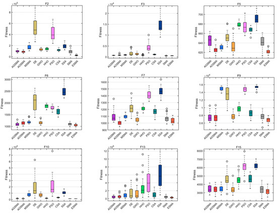
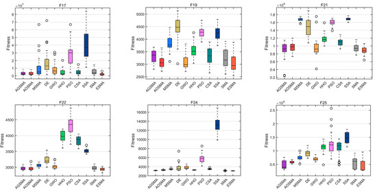
Figure 9.
Fifty-dimensional boxplot of each comparison algorithm.
Table 6 shows a comparison of the mean, best, and standard deviation results obtained by each algorithm computed on the 29 CEC2017 benchmark functions when the dimension is 100 Dim. With increasing dimension, the performance of the ESMA remains consistently stable. It achieves the first rank in 19 functions including F1, F3, F6, F10–F14, and F24–F29, among others. The rank of Friedman’s test is calculated to be 1.5172. These results highlight the ability of the ESMA to effectively tackle high-dimensional problems, showcasing its exceptional stability and robustness. Among the 11 participating randomized search algorithms, the ESMA proves to be the top-performing method. In contrast, the standard SMA demonstrates weaker performance compared to the ESMA. It fails to achieve the best solution for any function and obtains a Friedman mean rank value of 3.7241, ranking fourth among the eleven algorithms. The aforementioned results demonstrate that the novel global exploration approach, lens mapping learning with dynamic parameters and dimensional reorganization using vertical and horizontal crossover, effectively solves and surpasses the limitations of the standard SMA, particularly in high-dimensional scenarios.

Table 6.
Result of the ESMA 100 Dim on CEC2017 functions.
The performance of the other variants of SMA, namely AGSMA, AOSMA, and MSMA, demonstrates a decreasing trend. AGSMA outperforms the other variants in four functions, while AOSMA excels in five functions and MSMA demonstrates superiority in one function. The corresponding Friedman mean rank values are 2.8276, 3.5172, and 6.4138, respectively.
Among six other standard stochastic search algorithms, namely GWO, DE, HHO, PSO, CSA, and SSA, the ESMA exhibits the lowest mean value for all functions. However, except for ESMA, it is worth noting that GWO outperforms all other standard stochastic search algorithms in terms of optimization performance. The mean values demonstrate that the ESMA improves the performance of the other algorithms to varying degrees across different types of benchmark function optimizations. Furthermore, the ESMA also demonstrates superior test results in terms of robustness and effectiveness, as indicated by the Std and Best values.
In conclusion, the ESMA has successfully enhanced both the convergence speed and optimization accuracy through improvements in population diversity and prevention of local optimization.
4.3. CEC2013-Based Effectiveness Analysis
Table 7 shows the benchmark function optimization results of the ESMA and other comparative algorithms in 11 CEC2013-based 30-dimensional problems. From the Mean and Std values in the table, it is evident that the ESMA achieves the highest ranking for the two unimodal functions. The ESMA outperforms other comparative algorithms in terms of optimization accuracy and solution stability. These findings prove that the ESMA exhibits superior performance in unimodal function optimization compared to the standard SMA and other algorithms used in the test. The slime mould individuals demonstrate effective exploration of the solution space, resulting in improved optimization outcomes. The optimization performance of the algorithms is significantly challenged when dealing with the basic multimodal and composition functions F32–F40, which contain numerous local minima. In this regard, the ESMA demonstrates superior convergence accuracy compared to other comparative algorithms, while also exhibiting higher algorithmic stability. The ESMA also achieves the best results in F30–F34 and F36–F39 for the Best value, surpassing other SMA variants and non-SMA algorithms. This suggests that the ESMA test algorithm performs exceptionally well even in extreme scenarios. Only in the case of F35, do we observe that the optimization accuracy of the ESMA is slightly lower than that of the AOSMA. However, in the overall function test, the ESMA achieves a Friedman mean rank of 1.4545, indicating that it is the top-performing algorithm for most functions. This shows that the optimization ability of the ESMA can be further enhanced through multi-strategy improvement.

Table 7.
Result of the ESMA 30Dim on CEC2013 functions.
Table 8 presents the results of optimizing functions in 100 dimensions for each algorithm. In the case of all 11 functions, the ESMA consistently achieves superior optimization accuracy as well as better solution stability. These findings suggest that, even with the incorporation of multiple improvement strategies, the optimization ability of the ESMA does not diminish as the dimension of the function increases. Thus, the ESMA consistently delivers good optimization results.

Table 8.
Result of the ESMA 100Dim on CEC2013 functions.
4.4. Execution Time
Table 9 shows the execution time of each algorithm involved for dimensions ranging from 30 to 100. The calculation is performed by executing the 29 functions of CEC2017 and the 11 functions of CEC2013 independently for each algorithm, repeating the process 30 times. The maximum number of iterations is set to 1000. The table indicates a distinction between the improved and unimproved algorithms, with the former generally requiring more time than the latter. This discrepancy arises from the fact that the improved algorithm necessitates modifications to the formula structure, as well as the inclusion of additional strategies, in order to enhance its performance. Among the unimproved algorithms, HHO takes the longest time due to its numerous update methods, while PSO and CSA require less time as they rely on a smaller number of simpler update methods. The second highest time consumption is observed in the SMA, which is attributed to the presence of three update methods involving the calculation of fitness values for the weights, , and the need for sequencing. Among the improved algorithms, the MSMA has the highest time consumption, followed by the ESMA which has a similar time consumption to the AOSMA. It is worth noting that the AOSMA incorporates only one contrastive learning method, whereas the ESMA incorporates three methods, yet achieves a comparable time cost. In comparison to the MSMA, the ESMA exhibits significantly lower time consumption, despite both algorithms incorporating three strategies. In summary, the ESMA utilizes multiple strategies to enhance the SMA, which incurs a certain amount of execution time but achieves optimal optimization search capability compared to other algorithms.

Table 9.
Execution time/s spent on each algorithm.
4.5. Atatistical Test
Table 10 displays the p-values, which serve as an essential indicator for determining the presence of a significant difference between the algorithms. A p-value below 0.01 indicates a significant difference in the data. In the case of the ESMA, the asymptotic significance of the p-value is consistently below 0.01 for the 30 Dim, 50 Dim, and 100 Dim scenarios, suggesting a significant difference in performance compared to other algorithms. This variability is likely attributed to the three improvement strategies implemented by the ESMA.

Table 10.
Asymptotic results of Friedman’s test.
4.6. ESMA Diversity Analysis
The conducted experiments successfully passed the CEC2017 and CEC2013 benchmarks, encompassing a total of 40 functions tested in various directions. The experimental results demonstrate that the ESMA exhibited favorable optimization-seeking capabilities. This subsection aims to investigate the algorithm’s dimensional diversity during the iterative process. Hussain [62] emphasizes the equal importance of thoroughly exploring the diversity of algorithms and studying performance metrics, such as mean and variance. The key distinction is that the former specifically focuses on analyzing the behavioral state of each searching individual within the entire population.
In this paper, we adopt Hussain’s proposed method of measuring dimensional diversity to investigate the behavioral state of slime mould individuals in the ESMA. Equations (30) and (31) show this method.
where is the median of dimension j in the whole population, and is the dimension of the slime mould individual , and is the size of the population. is the mean of the dimensions of the searched individuals, and is the mean of the diversity of all dimensions.
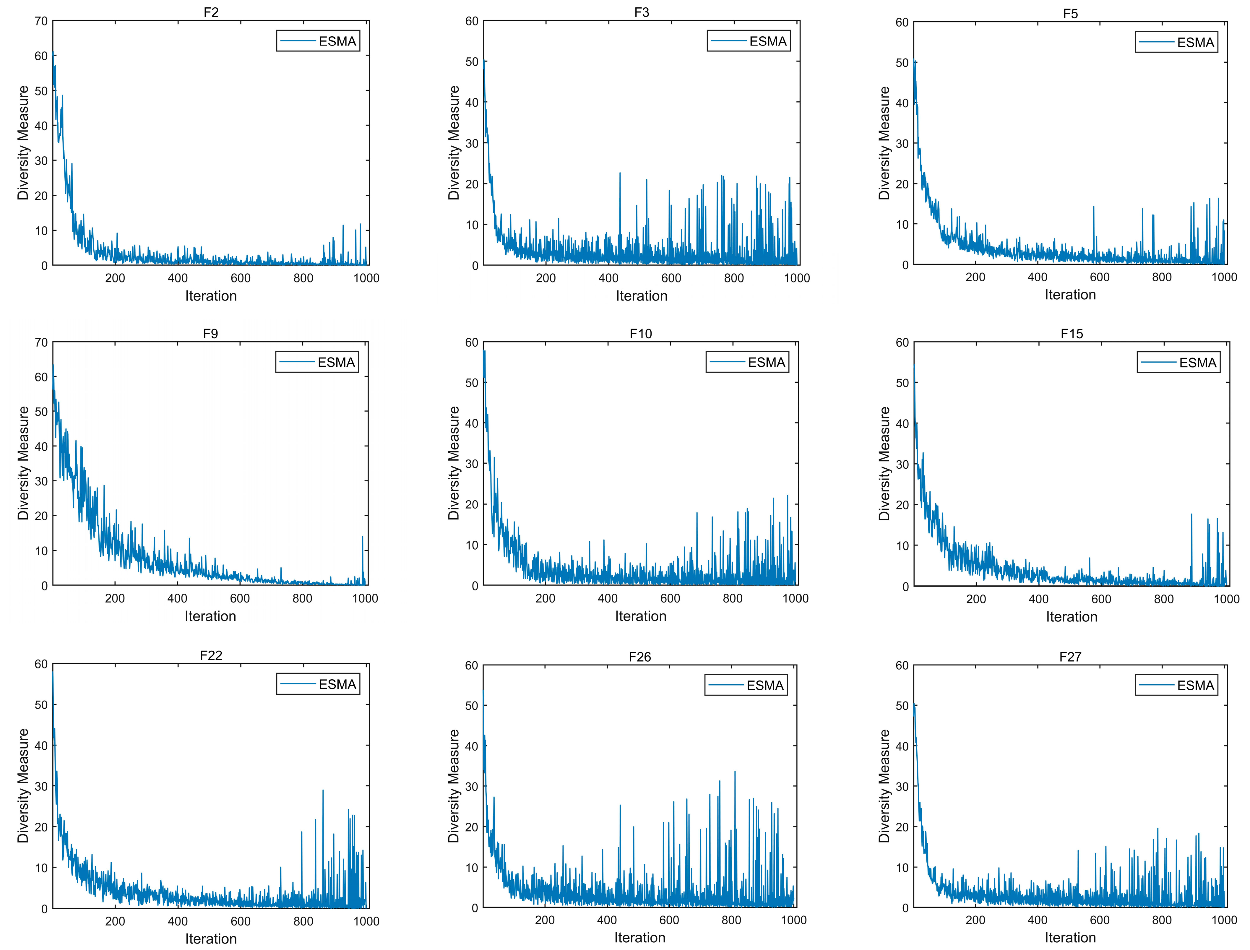
To comprehensively demonstrate the diversity of the ESMA, Figure 10 presents the dimensional diversity curves obtained by calculating the nine CEC2017 functions, including unimodal, multimodal, hybrid, and composition functions, with a dimension of 30. The figure illustrates that the amalgamation of various improvement strategies enables the algorithm to maintain a favorable population diversity. In the stage of global exploration, each function exhibits significant diversity, facilitating improved exploration of unknown regions in the entire search space. With an increasing number of iterations, the ESMA continues to maintain strong population diversity in functions such as multimodal F3 and composition function F26, enabling it to identify best solutions during local searching.
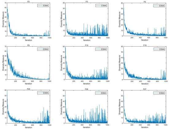
Figure 10.
Diversity measurement for the ESMA.
4.7. ESMA Exploration and Exploitation Analysis
This part of the experiment builds upon the previously described measurements of algorithmic diversity. It quantifies the relationship between exploration and development, highlighting the importance of balancing global and local searches in achieving effective search performance. The specific calculations can be found in Ref. [62] and are detailed in Equations (32) and (33).
where and are the percentages of exploration and exploitation, respectively, and is the maximum diversity of the population.
Figure 11 presents the results of the ESMA’s computation of the exploration and exploitation percentages for the nine functions in CEC2017 under 30 Dim.
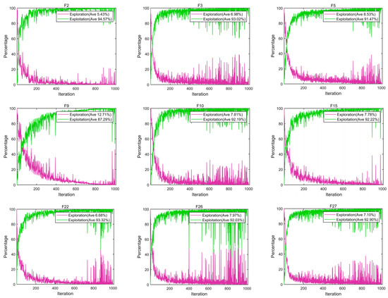
Figure 11.
Curves of exploitation and exploration rates for the ESMA.
From the figure, it can be observed that the algorithm exhibits a high percentage of the exploitation process, which is based on its ability to extensively search unknown regions in the global exploration mode.
Specifically, the average exploitation percentages for unimodal F2, multimodal F3, and composition F22 are remarkably high at 94.57%, 93.02%, and 93.32%, respectively. This enables the ESMA to achieve improved approximation results for the problem. Furthermore, when confronted with other complex, multidimensional, and multimodal problems, the ESMA maintains an appropriate exploration percentage, effectively enhancing its ability to prevent premature convergence in the early stage of the algorithm. In conclusion, the ESMA effectively strikes a balance between global exploration and local exploitation.
4.8. Real-World Engineering Problems
All stochastic search algorithms are developed and enhanced with the aim of solving real-world problems. In the previous test, their effectiveness was examined through numerical experiments. In this subsection, the ESMA method is applied to evaluate the exploration and exploitation capabilities in real-world scenarios. To ensure fairness, the experimental environment for these engineering problems remains consistent with the numerical tests.
4.8.1. Robot Path Planning Problem
Robot path planning plays a crucial role in various fields, including agricultural production, underwater operations, air transportation, etc.
Hao et al. [63] utilized a genetic algorithm (GA) to address the obstacle avoidance problem of an underwater autonomous underwater vehicle (AUV). On the other hand, Song et al. [64] applied an ant colony optimization (ACO) algorithm to solve the path planning issue encountered by a coal mining robot.
In this paper, we take the classic two-dimensional path selection problem of a robot as an illustrative example to discuss the application of the ESMA. It is assumed that in path planning, the movement of each searching individual from the starting point to the end point is considered a feasible path. The environment modeling employs the grid method to construct a map matrix, denoted as , with a size of m × n and each element occupying a space of . The robot’s movement should be within the 2D map and limited by obstacles. Obstacles at equivalent locations are computed based on the elements of matrix . Element 0 is noted as a feasible node and 1 is noted as an obstacle region. The robot can move on the grid with element value 0. The dimension represents the column subscripts in . The path planning objective is to search for the shortest movement distance of an individual, so its length can be expressed as Equation (34):
In this path planning test, a total of seven algorithms, including the AOSMA, AOA [65], GWO, DE, PSO, CSA, and SMA, were compared with the ESMA. The parameters for AOA were set according to the original literature, while the parameters for other algorithms remained consistent with Table 2. The population size was set to 30, and the number of iterations was set to 20. Each algorithm was run independently 30 times. The map size was set to . The best distance and average distance of each algorithm test results were recorded, and rankings were assigned based on these values.
From the statistical data in Table 11, it is shown that the ESMA achieves the shortest distance and average distance among all algorithms in the case of obstacle avoidance. The best distance measures 29.7989 and the average distance measures 29.8109, ranking the ESMA in the first position. This indicates that the path planned by the ESMA demonstrates excellent stability. The standard SMA ranks second, with the best distance of 29.9159 and an average distance of 29.8989, both of which are larger than those of the ESMA. AOSMA, AOA, GWO, DE, PSO, and CSA rank third, sixth, seventh, fifth, fourth, and eighth, respectively, all performing weaker than the ESMA. Figure 12 illustrates the trajectory of each participating algorithm mentioned above. It can be observed that ESMA exhibits superior obstacle avoidance capabilities and achieves the shortest path.

Table 11.
Comparison results of the path planning problem.
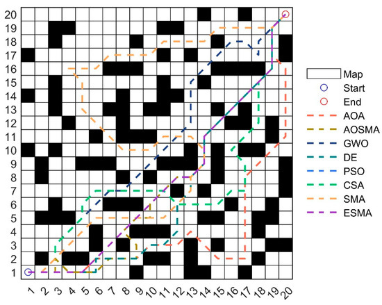
Figure 12.
Movement paths for each algorithm.
4.8.2. Pressure Vessel Design Problem
The objective of pressure vessel design (PVD) [66] is to minimize the cost of manufacturing (including pairing, forming, and welding) the pressure vessel while meeting the required specifications. The design, as shown in Figure 13, includes covers at both ends of the pressure vessel, with the cover at the head end being semi-spherical in shape. is the cross-sectional length of the cylindrical portion of the head without considering the head, and is the diameter of the inner wall of the cylindrical portion, and Th denote the wall thickness of the cylindrical part and the wall thickness of the head, respectively. , , , and are the four optimization variables of the pressure vessel design problem. The objective function of the problem and the four optimization constraints are shown in Equations (35)–(41).
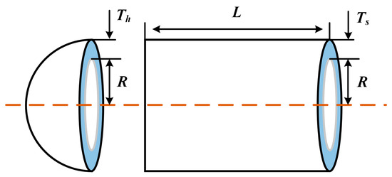
Figure 13.
Pressure vessel design.
The constraints are as follows:
The ESMA is compared with the AGWO [66], WOA, ALO [67], PSO, PIO, and SMA, each of which is implemented based on the original literature. According to the results presented in Table 12, the ESMA outperforms all other algorithms in solving the pressure vessel design problem, achieving the lowest total cost.

Table 12.
Comparison results of the PVD problem.
5. Summary and Future
This paper introduces a modification to the global exploration phase of the SMA in order to improve aimless random exploration with positive and negative feedback. The improved approach, utilizing the Lévy flight technique with selective average position and jumping, enhances the global optimality seeking performance of the ESMA compared to the original operation. The introduction of a dynamic lens mapping learning strategy improves the position of the leader individual and its ability to escape local optima. Additionally, incorporating a vertical and horizontal crossover between dimensions to rearrange the current individuals during each iteration promotes population diversity. The performance of the ESMA was assessed by employing a set of 40 functions from CEC2017 and CEC2013, which yielded favorable numerical results across various metrics such as Best, Mean, Standard Deviation, and the Friedman test. Furthermore, the ESMA demonstrates its superiority in addressing two classical real-world problems: path planning and pressure vessel design.
In future research, it is worth exploring the applicability of the ESMA to a wider range of engineering problems, including but not limited to imaging and chemistry, in order to expand its utilization. Furthermore, integrating the ESMA with other approaches can facilitate the development of more valuable and improved versions.
Author Contributions
Conceptualization, W.X. and D.L.; methodology, W.X. and D.L.; software, W.X.; validation, W.X., D.L. and D.Z.; formal analysis, W.X. and D.L.; investigation, W.X. and D.L.; resources, D.L. and D.Z.; data curation, W.X. and D.L.; writing—original draft preparation, W.X.; writing—review and editing, Z.L.; visualization, R.L.; supervision, D.L. and Z.L.; project administration, D.L.; funding acquisition, W.X. All authors have read and agreed to the published version of the manuscript.
Funding
This research received no external funding.
Data Availability Statement
Not applicable.
Conflicts of Interest
The authors declare no conflict of interest.
References
- Si, T.; Patra, D.K.; Mondal, S.; Mukherjee, P. Breast DCE-MRI segmentation for lesion detection using Chimp Optimization Algorithm. Expert Syst. Appl. 2022, 204, 117481. [Google Scholar] [CrossRef]
- Huiling, C.; Shan, J.; Mingjing, W.; Asghar, H.A.; Xuehua, Z. Parameters identification of photovoltaic cells and modules using diversification-enriched Harris hawks optimization with chaotic drifts. J. Clean. Prod. 2020, 244, 118788. [Google Scholar]
- Zhu, D.; Huang, Z.; Liao, S.; Zhou, C.; Yan, S.; Chen, G. Improved Bare Bones Particle Swarm Optimization for DNA Sequence Design. IEEE Trans. NanoBiosci. 2023, 22, 603–613. [Google Scholar] [CrossRef]
- Yan, Z.; Wang, J.; Li, G.C. A collective neurodynamic optimization approach to bound-constrained nonconvex optimization. Neural Netw. Off. J. Int. Neural Netw. Soc. 2014, 55, 20–29. [Google Scholar] [CrossRef]
- Sahoo, S.K.; Saha, A.K. A Hybrid Moth Flame Optimization Algorithm for Global Optimization. J. Bionic Eng. 2022, 19, 1522–1543. [Google Scholar] [CrossRef]
- Chen, X.; Tang, B.; Fan, J.; Guo, X. Online gradient descent algorithms for functional data learning. J. Complex. 2022, 70, 101635. [Google Scholar] [CrossRef]
- Neculai, A. A diagonal quasi-Newton updating method for unconstrained optimization. Numer. Algorithms 2019, 81, 575–590. [Google Scholar]
- Bellet, J.-B.; Croisille, J.-P. Least squares spherical harmonics approximation on the Cubed Sphere. J. Comput. Appl. Math. 2023, 429, 115213. [Google Scholar] [CrossRef]
- Bader, A.; Randa, A.; Hafez, E.H.; Riad Fathy, H. On the Mixture of Normal and Half-Normal Distributions. Math. Probl. Eng. 2022, 2022, 3755431. [Google Scholar]
- Natido, A.; Kozubowski, T.J. A uniform-Laplace mixture distribution. J. Comput. Appl. Math. 2023, 429, 115236. [Google Scholar] [CrossRef]
- Laith, A.; Ali, D.; Woo, G.Z. A Comprehensive Survey of the Harmony Search Algorithm in Clustering Applications. Appl. Sci. 2020, 10, 3827. [Google Scholar]
- Abualigah, L.; Yousri, D.; Abd Elaziz, M.; Ewees, A.A.; Al-Qaness, M.A.; Gandomi, A.H. Aquila Optimizer: A novel meta-heuristic optimization algorithm. Comput. Ind. Eng. 2021, 157, 107250. [Google Scholar] [CrossRef]
- Wang, G.G.; Deb, S.; Cui, Z.H. Monarch butterfly optimization. Neural Comput. Appl. 2019, 31, 1995–2014. [Google Scholar] [CrossRef]
- Kaveh, A.; Dadras, A. A novel meta-heuristic optimization algorithm: Thermal exchange optimization. Adv. Eng. Softw. 2017, 110, 69–84. [Google Scholar] [CrossRef]
- Seyedali, M.; Andrew, L. The Whale Optimization Algorithm. Adv. Eng. Softw. 2016, 95, 51–67. [Google Scholar]
- Gaurav, D.; Vijay, K. Seagull optimization algorithm: Theory and its applications for large-scale industrial engineering problems. Knowl.-Based Syst. 2019, 165, 169–196. [Google Scholar]
- Duan, H.; Qiao, P. Pigeon-inspired optimization: A new swarm intelligence optimizer for air robot path planning. Int. J. Intell. Comput. Cybern. 2014, 7, 24–37. [Google Scholar] [CrossRef]
- Asghar, H.A.; Seyedali, M.; Hossam, F.; Ibrahim, A.; Majdi, M.; Chen, H. Harris hawks optimization: Algorithm and applications. Future Gener. Comput. Syst. 2019, 97, 849–872. [Google Scholar]
- Baykasoglu, A.; Ozsoydan, F.B. Adaptive firefly algorithm with chaos for mechanical design optimization problems. Appl. Soft Comput. 2015, 36, 152–164. [Google Scholar] [CrossRef]
- Zhu, D.; Wang, S.; Zhou, C.; Yan, S. Manta ray foraging optimization based on mechanics game and progressive learning for multiple optimization problems. Appl. Soft Comput. 2023, 145, 110561. [Google Scholar] [CrossRef]
- Bhargava, G.; Yadav, N.K. Solving combined economic emission dispatch model via hybrid differential evaluation and crow search algorithm. Evol. Intell. 2022, 15, 1161–1169. [Google Scholar] [CrossRef]
- Li, S.; Chen, H.; Wang, M.; Asghar, H.A.; Seyedali, M. Slime mould algorithm: A new method for stochastic optimization. Future Gener. Comput. Syst. 2020, 111, 300–323. [Google Scholar] [CrossRef]
- Zhou, X.; Chen, Y.; Wu, Z.; Heidari, A.A.; Chen, H.; Alabdulkreem, E.; Escorcia-Gutierrez, J.; Wang, X. Boosted local dimensional mutation and all-dimensional neighborhood slime mould algorithm for feature selection. Neurocomputing 2023, 551, 126467. [Google Scholar] [CrossRef]
- Wolpert, D.H.; Macready, W.G. No free lunch theorems for optimization. IEEE Trans. Evol. Comput. 1997, 1, 67–82. [Google Scholar] [CrossRef]
- Deng, L.; Liu, S. An enhanced slime mould algorithm based on adaptive grouping technique for global optimization. Expert Syst. Appl. 2023, 222, 119877. [Google Scholar] [CrossRef]
- Kumar, N.M.; Pand; Rutuparna; Ajith, A. Adaptive opposition slime mould algorithm. Soft Comput. 2021, 25, 14297–14313. [Google Scholar]
- Deng, L.; Liu, S. A multi-strategy improved slime mould algorithm for global optimization and engineering design problems. Comput. Methods Appl. Mech. Eng. 2023, 404, 116200. [Google Scholar] [CrossRef]
- Storn, R.; Price, K. Differential Evolution—A Simple and Efficient Heuristic for global Optimization over Continuous Spaces. J. Glob. Optim. 1997, 11, 341–359. [Google Scholar] [CrossRef]
- Kennedy, J.; Eberhart, R. Particle swarm optimization. In Proceedings of the IEEE International Conference on Neural Networks—Conference Proceedings, Perth, WA, Australia, 27 November–1 December 1995. [Google Scholar]
- Seyedali, M.; Mohammad, M.S.; Andrew, L. Grey Wolf Optimizer. Adv. Eng. Softw. 2014, 69, 46–61. [Google Scholar]
- Mirjalili, S.; Gandomi, A.H.; Mirjalili, S.Z.; Saremi, S. Salp swarm algorithm: A bio-inspired optimizer for engineering design problems. Adv. Eng. Softw. 2017, 114, 163–191. [Google Scholar] [CrossRef]
- Alireza, A. A novel metaheuristic method for solving constrained engineering optimization problems: Crow search algorithm. Comput. Struct. 2016, 169, 1–12. [Google Scholar]
- Hong, M.; Zhongrui, Q.; Chengbi, Z. Multi-Strategy Improved Slime Mould Algorithm and its Application in Optimal Operation of Cascade Reservoirs. Water Resour. Manag. 2022, 36, 3029–3048. [Google Scholar]
- Altay, O. Chaotic slime mould optimization algorithm for global optimization. Artif. Intell. Rev. 2022, 55, 3979–4040. [Google Scholar] [CrossRef]
- Tang, A.D.; Tang, S.Q.; Han, T.; Zhou, H.; Xie, L. A Modified Slime Mould Algorithm for Global Optimization. Comput. Intell. Neurosci. 2021, 2021, 2298215. [Google Scholar] [CrossRef]
- Gao, Z.-M.; Zhao, J.; Li, S.-R. The Improved Slime Mould Algorithm with Cosine Controlling Parameters. J. Phys. Conf. Ser. 2020, 1631, 012083. [Google Scholar] [CrossRef]
- Hu, J.; Gui, W.; Asghar, H.A.; Cai, Z.; Liang, G.; Chen, H.; Pan, Z. Dispersed foraging slime mould algorithm: Continuous and binary variants for global optimization and wrapper-based feature selection. Knowl.-Based Syst. 2022, 237, 107761. [Google Scholar] [CrossRef]
- Karaboga, D.; Basturk, B. On the performance of artificial bee colony (ABC)algorithm. Appl. Soft Comput. 2008, 8, 687–697. [Google Scholar] [CrossRef]
- Rizk-Allah, R.M.; Hassanien, A.E.; Song, D. Chaos-opposition-enhanced slime mould algorithm for minimizing the cost of energy for the wind turbines on high-altitude sites. ISA Trans. 2022, 121, 191–205. [Google Scholar] [CrossRef]
- Ren, L.; Heidari, A.A.; Cai, Z.; Shao, Q.; Liang, G.; Chen, H.L.; Pan, Z. Gaussian kernel probability-driven slime mould algorithm with new movement mechanism for multi-level image segmentation. Measurement. J. Int. Meas. Confed. 2022, 192, 110884. [Google Scholar] [CrossRef]
- Ahmadianfar, I.; Noori, R.M.; Togun, H. Multi-strategy Slime Mould Algorithm for hydropower multi-reservoir systems optimization. Knowl.-Based Syst. 2022, 250, 109048. [Google Scholar] [CrossRef]
- Pawani, K.; Singh, M. Combined Heat and Power Dispatch Problem Using Comprehensive Learning Wavelet-Mutated Slime Mould Algorithm. Electr. Power Compon. Syst. 2023, 51, 12–28. [Google Scholar] [CrossRef]
- Sun, K.; Jia, H.; Li, Y.; Jiang, Z. Hybrid improved slime mould algorithm with adaptive β hill climbing for numerical optimization. J. Intell. Fuzzy Syst. 2020, 40, 1667–1679. [Google Scholar] [CrossRef]
- Zhong, C.; Li, G.; Meng, Z. A hybrid teaching–learning slime mould algorithm for global optimization and reliability-based design optimization problems. Neural Comput. Appl. 2022, 34, 16617–16642. [Google Scholar] [CrossRef]
- Liu, L.; Zhao, D.; Yu, F.; Heidari, A.A.; Ru, J.; Chen, H.; Mafarja, M.; Turabieh, H.; Pan, Z. Performance optimization of differential evolution with slime mould algorithm for multilevel breast cancer image segmentation. Comput. Biol. Med. 2021, 138, 104910. [Google Scholar] [CrossRef]
- Izci, D.; Ekinci, S.; Zeynelgil, H.L.; Hedley, J. Fractional Order PID Design based on Novel Improved Slime Mould Algorithm. Electr. Power Compon. Syst. 2022, 49, 901–918. [Google Scholar] [CrossRef]
- Kirkpatrick, S.; Gelatt, C.D.; Vecchi, M.P. Optimization by simulated annealing. Science 1983, 220, 671–680. [Google Scholar] [CrossRef]
- Nafi, Ö.B.; Berkan, A.S.; Timur, D.; Bilal, Ö. A novel version of slime mould algorithm for global optimization and real world engineering problems Enhanced slime mould algorithm. Math. Comput. Simul. 2022, 198, 253–288. [Google Scholar]
- Mirjalili, S. SCA: A Sine Cosine algorithm for Solving Optimization Problems. Knowl.-Based Syst. 2016, 96, 120–133. [Google Scholar] [CrossRef]
- Yin, S.; Luo, Q.; Zhou, Y. EOSMA: An Equilibrium Optimizer Slime Mould Algorithm for Engineering Design Problems. Arab. J. Sci. Eng. 2022, 47, 10115–10146. [Google Scholar] [CrossRef]
- Faramarzi, A.; Heidarinejad, M.; Stephen, B.; Mirjalili, S. Equilibrium optimizer: A novel optimization algorithm. Knowl.-Based Syst. 2020, 191, 105190. [Google Scholar] [CrossRef]
- Tang, H.; Fang, B.; Liu, R. A hybrid teaching and learning-based optimization algorithm for distributed sand casting job-shop scheduling problem. Appl. Soft Comput. 2022, 120, 108694. [Google Scholar] [CrossRef]
- Joshi, S.K. Levy flight incorporated hybrid learning model for gravitational search algorithm. Knowl.-Based Syst. 2023, 265, 110374. [Google Scholar] [CrossRef]
- Ewees Ahmed, A.; Mostafa Reham, R.; Ghoniem Rania, M.; Gaheen Marwa, A. Improved seagull optimization algorithm using Lévy flight and mutation operator for feature selection. Neural Comput. Appl. 2022, 34, 7437–7472. [Google Scholar] [CrossRef]
- Park, S.-Y.; Lee, J.-J. Stochastic opposition-based learning using a beta distribution in differential evolution. IEEE Trans. Cybern. 2016, 46, 2184–2194. [Google Scholar] [CrossRef]
- Yu, X.; Xu Wang, Y.; Li, C.-L. Opposition-based learning grey wolf optimizer for global optimization. Knowl.-Based Syst. 2021, 226, 107139. [Google Scholar] [CrossRef]
- Long, W.; Jiao, J.; Xu, M. Lens-imaging learning Harris hawks optimizer for global optimization and its application to feature selection. Expert Syst. Appl. 2022, 202, 117255. [Google Scholar] [CrossRef]
- Han, M.; Du, Z.; Zhu, H.; Li, Y.; Yuan, Q.; Zhu, H. Golden-Sine dynamic marine predator algorithm for addressing engineering design optimization. Expert Syst. Appl. 2022, 210, 118460. [Google Scholar] [CrossRef]
- Yue, S.; Zhang, H. A hybrid grasshopper optimization algorithm with bat algorithm for global optimization. Multimed. Tools Appl. 2021, 80, 3863–3884. [Google Scholar] [CrossRef]
- Meng, A.B.; Chen, Y.C.; Yin, H.; Chen, S.Z. Crisscross optimization algorithm and its application. Knowl.-Based Syst. 2014, 67, 218–229. [Google Scholar] [CrossRef]
- Mohamed, A.; Mohamed, A. Adaptive guided differential evolution algorithm with novel mutation for numerical optimization. Int. J. Mach. Learn. Cybern. 2019, 10, 253–277. [Google Scholar] [CrossRef]
- Kashif, H.; Mohd, S.M.N.; Cheng, S.; Shi, Y. On the exploration and exploitation in popular swarm-based metaheuristic algorithms. Neural Comput. Appl. 2019, 31, 7665–7683. [Google Scholar]
- Hao, K.; Zhao, J.; Li, Z.; Liu, Y.; Zhao, L. Dynamic path planning of a three-dimensional underwater AUV based on an adaptive genetic algorithm. Ocean Eng. 2022, 263, 112421. [Google Scholar] [CrossRef]
- Song, B.; Miao, H.; Xu, L. Path planning for coal mine robot via improved ant colony optimization algorithm. Syst. Sci. Control Eng. 2021, 9, 283–289. [Google Scholar] [CrossRef]
- Hashim, F.A.; Hussain, K.; Houssein, E.H.; Mabrouk, M.S.; Al-Atabany, W. Archimedes optimization algorithm: A new metaheuristic algorithm for solving optimization problems. Appl. Intell. 2021, 51, 1531–1551. [Google Scholar] [CrossRef]
- Ma, C.; Huang, H.; Fan, Q. Grey wolf optimizer based on Aquila exploration method. Expert Syst. Appl. 2022, 205, 117629. [Google Scholar] [CrossRef]
- Mirjalili, S. The Ant Lion Optimizer. Adv. Eng. Softw. 2015, 83, 80–98. [Google Scholar] [CrossRef]
Disclaimer/Publisher’s Note: The statements, opinions and data contained in all publications are solely those of the individual author(s) and contributor(s) and not of MDPI and/or the editor(s). MDPI and/or the editor(s) disclaim responsibility for any injury to people or property resulting from any ideas, methods, instructions or products referred to in the content. |
© 2023 by the authors. Licensee MDPI, Basel, Switzerland. This article is an open access article distributed under the terms and conditions of the Creative Commons Attribution (CC BY) license (https://creativecommons.org/licenses/by/4.0/).


