A PDE Model Approach to Formation Control of Large-Scale Mobile Sensor Networks with Boundary Uncertainties

Abstract

This paper investigates the formation problem of an array of large-scale mobile sensor networks. A new framework for the dynamic of mobile sensors as a continuum described by the parabolic system with boundary disturbance is proposed. The communication topology of agents is a chain graph and fixed. Leader feedback laws which are designed in a manner to the boundary control of large-scale mobile sensor networks allow the mobile sensors to achieve the formation steadily. By referring to the Lyapunov functional method and employing a boundary control approach, a new protocol is established to deal with a formation problem for the large-scale mobile sensor networks. Finally, numerical examples are given to illustrate the usefulness of the results.

1. Introduction

During the last few decades, wireless sensor networks have been intensively explored and applied in a wide variety of fields [1,2], including military, surroundings, health, and home. A collection of sensing devices which are connected by wireless communication can be built into a wireless sensor network in engineering. In order to adapt to the requirement of flexibility in applications, the sensing nodes of wireless sensor networks can be endowed mobility using mobile devices. Mobile sensing devices reduce power consumption and costs while also improving performance. In the last few years, mobile sensor networks have attracted a lot more interest because they have been successful in a wide range of applications including formation control [3,4,5], target tracking [6,7,8], environmental monitoring [9,10], and other areas. The study of cooperative control of mobile sensing networks has been viewed as a crucial issue.

Ref. [11] presents a robust control system for mobile sensors moving collaboratively in a distributed environment. A gradient climbing task in which mobile sensor networks can adapt its configuration in response to the measured environment. In [12], three distributed stable deployment algorithms based on flocking in mobile sensor networks are addressed. In addition, from the view of swarm, the control problem of wireless sensor networks with mobile multi-robots is discussed in [13,14]. Moreover, formation control of mobile sensor networks has been investigated intensively. A distributed control model is given to form the desired formation in [15]. The distributed observers are studied to achieve the formation in [16]. Stabilization of geometric pattern based on Laplacian are considered in [8,9,17]. Deployment onto a desired planar curve is investigated in [18] and [19] using coverage control algorithms and Lie group setting, respectively.

In general, the model suggested in [20] or versions of these models are used in the majority of studies concerning mobile sensor networks models. The model presented by Reynolds contains three heuristic rules. They are alignment, cohesion, and separation. Some additional rules such as obstacle avoidance capabilities have been suggested ever since. It is not difficult to see that these models are the particle system essentially. The discrete dynamic characteristics are exhibited in these models. Nevertheless, an increasing number of studies have found that continuity and layered property exist in biological systems [21], social systems and so on. In [21], the authors proposed the starling swarm coordination for studying the behavior inertia and information transfer of the birds, which could study the cooperative flight of unmanned aerial vehicle. These phenomena show us that the system should be interpreted as a continuum when it is made up of a significant number of mobile sensing devices. That is to say, large-scale mobile sensor networks(LMSNs) is a fluid instead of a particle system. Therefore, the large-scale mobile sensor networks should be modeled as a partial differential equation (PDE).

For the past few years, a partial differential equation has been an effective tool that begins to analyze the multi-agent system [22,23,24]. In particular, [22] used the LWR equation for crowd evacuation, Ref. [23] analyzes the stability of vehicular platoons based on an unstable hyperbolic system, and Ref. [24] models multi-agents as reaction–advection–diffusion equations for deployment onto spatial curves. Furthermore, growing results of experiments suggest that the partial differential equation has gradually become an important way of system modeling. However, it should be pointed out that a PDE-based model for formation control of large-scale mobile sensor networks still has little research attention.

Therefore, the major purpose of this research is to investigate the formation issue for an array of large-scale mobile sensor networks based on parabolic systems with boundary disturbance. For the PDE model of mobile sensor networks, the boundary control approach is addressed. Such a framework which implies the communication topology of mobile sensors is a chain graph and fixed. Hence, stable formation onto planar curves can be achieved by leaders, i.e., the boundary control of the leader such that mobile sensors will reach consensus. By constructing proper Lyapunov functional and employing the boundary control approach, some sufficient conditions have been established to cope with the formation issue for large group mobile sensing devices.

This study mainly contributes the following innovative points: (1) a framework for the dynamic of large-scale mobile sensors as a continuum and modeled by parabolic system is presented; (2) the design step about formation of large-scale mobile sensor networks is proposed; and (3) boundary disturbance in the larger group mobile sensing devices is considered. In order to exhibit the utility of the proposed boundary control strategy, numerical simulations are provided.

2. Problem Formulation and Preliminaries

In this study, a new framework is proposed for the dynamics of a large group of mobile sensors as a continuum by the parabolic system. Large-scale mobile sensor networks are moving in an obstacle-free two-dimensional plane. Energy constraints at the level of network nodes are not considered here. The dynamics of mobile sensor networks are described by the following integrator:

$$\frac{\partial x(\theta ,t)}{\partial t}=v(\theta ,t),$$

(1)

where $x(\theta ,t)={[x_1(\theta ,t),x_2(\theta ,t)]}^T$ denotes the position of agent $\theta$ at time t. The parameter $\theta$ as the identity of each mobile sensor in a large mobile sensor network, and $\theta \in [0,1]$. Namely, $\theta$ is a mobile sensor’s index code and as the spatial variable of mobile sensor network for the group’s collective dynamics. $v(\theta ,t)={[v_1(\theta ,t),v_2(\theta ,t)]}^T$ is the velocity for the agent $\theta$, and the control input $v(\theta ,t)$ is determined by

$$v(\theta ,t)=D\frac{{\partial }^{2}x(\theta ,t)}{\partial {\theta }^2},$$

(2)

with diffusion operator $D=\mathrm{diag}[d_1,d_2]$, constants $d_1,d_2$ are both positive.

The velocity input of diffusion-based feedback indicates all the agents utilize only local information from the nearest-neighbor. A distributed communication topology is given, which is a chain graph.

Remark 1.

It is worth mentioning that, in this paper, the input control (2) is given for the first-order integrator, which implies that this paper is studying the consensus of large-scale mobile sensor networks in the framework of the PDE model. In other words, this paper is concerned with the theoretical analysis of the collaborative dynamics of the system as a whole when the large-scale mobile nodes are viewed as a continuum (PDE model). The object of study here is the continuum, not the network.

The PDE model approach has natural advantages for the study of continuum models. However, the control inputs proposed in (2) in the paper also bring some limitations to the system model. In addition, (2) only considers the distributed chain communication topology of the system but does not describe phenomena such as output data missing, sensor saturation, or even node failure. These are currently being considered by the authors.

Remark 2.

In recent years, several important results about multi-agent system based on individual have been obtained. First-order integrator dynamics often can be presented as the model of multi-agent systems. The agent dynamics is expressed in the following:

$${\dot{x}}_i\left(t\right)=\sum _{j\in {\mathcal{N}}_i}(x_j\left(t\right)-x_i\left(t\right)),i=1,2,\cdots ,n,$$

where ${\mathcal{N}}_i$ is the set of neighbors that communicate with agent i. It is not difficult to obtain an associated continuum model by continuous approximation as follows:

$$\frac{\partial x(\theta ,t)}{\partial t}=\frac{{\partial }^{2}x(\theta ,t)}{\partial {\theta }^2},$$

where the velocity feedback of each agent(mobile sensor) employs the diffusion term.

The initial condition associated with (1) is given by

$$x(\theta ,0)=x_0\left(\theta \right),$$

(3)

where $x(\theta ,0)={[x_1(\theta ,0),x_2(\theta ,0)]}^T,x_0\left(\theta \right)={[x_{10}\left(\theta \right),x_{20}\left(\theta \right)]}^T$, and have the mixed boundary condition

$$x(0,t)={[0,0]}^T,\frac{\partial x(1,t)}{\partial \theta }=u\left(t\right)+w\left(t\right),$$

(4)

where $u\left(t\right)={[u_1\left(t\right),u_2\left(t\right)]}^T$ is the controls to be designed, $w\left(t\right)={[w_1\left(t\right),w_2\left(t\right)]}^T$ is an boundary disturbance, which assumes the following:

$${\int }_0^{+\infty }{w}^T\left(t\right)w\left(t\right)dt<+\infty .$$

(5)

It is worth mentioning that the initial condition should be compatible with the boundary condition, i.e.,

$$\frac{d{x}_0\left(\theta \right)}{d\theta }{|}_{\theta =0}=\mathbf{0},\frac{d{x}_0\left(\theta \right)}{d\theta }{|}_{\theta =1}=u\left(0\right)+w\left(0\right).$$

A large group of mobile sensors as a continuum by system (1), index $\theta =1$ is the leader sensor, and $\theta =0$ is the anchor sensor, the rest of index $0<\theta <1$ are the follower sensors. When proper boundary control law is designed such that ${lim}_{t\to +\infty }x(\theta ,t)=\overline{x}\left(\theta \right)$ for all $\theta \in [0,1]$, then mobile sensors are said to achieve formation consensus. Meanwhile, a large group of mobile sensors is also said to achieve consensus if $u\left(t\right)=\mathbf{0}$ for the leader.

Our main purpose in this paper is to accomplish the desired formation for an array of large mobile sensor networks based on heat equation with boundary disturbance by using the boundary control approach. Clearly, the 2D formation problem can be discussed in two aspects. On the one hand, what kind of formation can be reached by a continuum of mobile sensors under diffusion-based feedback? On the other hand, how can the boundary controller be designed such that mobile sensors steadily reach the formation?

3. Formation Control Scheme Design

First of all, we consider the diffusion-based feedback as velocity control input in continuum of mobile sensors. According to (1) and (2), the dynamics of mobile sensors are governed by heat equation

$$\frac{\partial x(\theta ,t)}{\partial t}=D\frac{{\partial }^{2}x(\theta ,t)}{\partial {\theta }^2}.$$

(6)

The equilibrium equation of (6) is a second ordinary differential equation

$$\frac{d^2\overline{x}\left(\theta \right)}{d{\theta }^2}=\mathbf{0}.$$

(7)

It is not difficult to solve the solution of (7) being a family of linear functions. Those functions can be decomposed to vertical and horizontal directions, respectively. The compact form of linear functions can be described as

$$\overline{x}\left(\theta \right)=\left[\begin{array}{c}{\overline{x}}_1\left(\theta \right)\\ {\overline{x}}_2\left(\theta \right)\end{array}\right]=\left[\begin{array}{cc}{a}_1& a_2\\ a_3& a_4\end{array}\right]\left[\begin{array}{c}1\\ \theta \end{array}\right],$$

(8)

where constants $a_1,a_2,a_3$ and $a_4$ are formation coefficients, which are picked by users to generate the shape of the target formation. The type of formation curve is determined by the basis $(1,\theta )$, which is the solution of (7). Therefore, mobile sensors which are governed by (6) have the capacity of achieving linear formations or rendezvousing at the origin.

Next, in general, the boundary control approach is an effective way for large mobile sensor networks described by parabolic systems. Thus, we consider the leader agent $(\theta =1)$ as boundary control input enabling large mobile sensors reach the desired formation stably. The control law of leader can be designed as follows:

$$u\left(t\right)=-Kx(1,t)+K\overline{x}\left(1\right)+\frac{d\overline{x}\left(1\right)}{d\theta },$$

(9)

where $x(1,t)={[x_1(1,t),x_2(1,t)]}^T$ and $\frac{d\overline{x}\left(1\right)}{d\theta }$ means $\frac{d\overline{x}\left(\theta \right)}{d\theta }{|}_{\theta =1}$.

To have mobile sensors successfully reach the formation, we shift the equilibrium $\overline{x}\left(\theta \right)$ to the origin by transformation $y(\theta ,t)=x(\theta ,t)-\overline{x}\left(\theta \right)$, and the formation error dynamics for mobile sensors can be obtained from (3), (4), and (6) as follows:

$$\begin{array}{cc}\hfill \frac{\partial y(\theta ,t)}{\partial t}=& D\frac{{\partial }^{2}y(\theta ,t)}{\partial {\theta }^2},\hfill \end{array}$$

(10)

$$\begin{array}{cc}\hfill y(\theta ,0)=& y_0\left(\theta \right),\hfill \end{array}$$

(11)

$$\begin{array}{cc}\hfill y(0,t)=& \mathbf{0},\frac{\partial y(1,t)}{\partial \theta }=U\left(t\right)+w\left(t\right),\hfill \end{array}$$

(12)

where $y(\theta ,t)={[y_1(\theta ,t),y_2(\theta ,t)]}^T$.

Substituting error $y(\theta ,t)$ into (4) and (8) leads to

$$U\left(t\right)=-Ky(1,t).$$

(13)

In brief, the design procedure of formation deployment of large mobile sensors is listed in the following:

• Find the equilibrium equation of dynamics model;
• Analyze the basis of equilibrium equation to determine the type of equilibrium curve component;
• Select the formation coefficients to determine the shape of equilibrium curve component;
• Orthogonal synthesis of the equilibrium curve of two coordinate axes to determine a target formation;
• Implement the control law for leader mobile sensor to achieve the formation.

4. Stability Analysis of the Closed-Loop System

To give our main results, we introduce the following definition and lemmas:

Definition 1

([25]). A parabolic system is said to be $L_2[0,1]$ stable, if

$$\underset{t\to +\infty }{lim}{\int }_0^1{y}^T(\theta ,t)y(\theta ,t)d\theta =\mathbf{0},$$

holds.

Definition 1 implies the closed-loop system state $x(\theta ,t)$ is $L_2[0,1]$ stable at the equilibrium curve $\overline{x}\left(\theta \right)$.

Definition 2

([26]). A parabolic system is said to be globally asymptotically stable, if

$$\underset{t\to +\infty }{lim}y(\theta ,t)=\mathbf{0},$$

holds.

Definition 2 implies ${lim}_{t\to +\infty }x(\theta ,t)=\overline{x}\left(\theta \right)$, that is to say, a large group of mobile sensors will converge into the formation $\overline{x}\left(\theta \right)$.

Lemma 1

([27]). Let $z\in W^{1,2}(a,b)$ be a scalar function with $z\left(a\right)=0$. Then,

$$\begin{array}{c}\hfill {\int }_a^b{z}^2\left(\xi \right)d\xi \le \frac{{(b-a)}^2}{2}{\int }_a^b{\left(\frac{dz\left(\xi \right)}{d\xi }\right)}^{2}d\xi ,\\ \hfill \underset{\xi \in [a,b]}{max}{z}^2\left(\xi \right)\le (b-a){\int }_a^b{\left(\frac{dz\left(\xi \right)}{d\xi }\right)}^{2}d\xi .\end{array}$$

Lemma 2

([25]). (The special case of Barbalat’s Lemma) Let $f\left(t\right)$ be a non-negative function defined on $[0,+\infty )$. If $f\left(t\right)$ is differentiable on $[0,+\infty )$ and ${sup}_{t\ge 0}\frac{df\left(t\right)}{dt}<+\infty$, and ${\int }_0^{+\infty }f\left(t\right)dt<+\infty$. Then, there holds

$$\underset{t\to +\infty }{lim}f\left(t\right)=0.$$

The following theorems present the main outcomes of the study.

4.1. Boundedness

Theorem 1.

Under the control scheme (13), the system (10) with boundary disturbance $w\left(t\right)$ satisfying (5) and the initial condition $y_0\left(\theta \right)$ satisfying ${\int }_0^{+\infty }{y}_0^T\left(\theta \right)y_0\left(\theta \right)d\theta <+\infty$ is uniformly square integrable, i.e.,

$$\underset{\theta \in [0,1]}{sup}{\int }_0^{+\infty }{y}^T(\theta ,t)y(\theta ,t)dt<+\infty ,$$

and ${\int }_0^1{y}^T(\theta ,t)y(\theta ,t)d\theta$ is bounded on $[0,+\infty )$ if ${\sigma }_2<{\sigma }_1$.

Proof. 

Consider a Lyapunov functional as

$$V\left(t\right)=\frac{1}{2}{\int }_0^1{y}^T(\theta ,t)y(\theta ,t)d\theta .$$

(14)

For the system (10), the time derivative of $V\left(t\right)$ can be computed as follows:

$$\begin{array}{cc}\hfill \frac{dV\left(t\right)}{dt}=& {\int }_0^1{y}^T(\theta ,t)\frac{\partial y(\theta ,t)}{\partial t}d\theta \hfill \\ \hfill =& {\int }_0^1{y}^T(\theta ,t)D\frac{{\partial }^{2}y(\theta ,t)}{\partial {\theta }^2}d\theta \hfill \\ \hfill =& y^T(\theta ,t)D\frac{\partial y(\theta ,t)}{\partial \theta }{|}_0^1\hfill \\ \hfill & -{\int }_0^1{\left(\frac{\partial y(\theta ,t)}{\partial \theta }\right)}^{T}D\frac{\partial y(\theta ,t)}{\partial \theta }d\theta \hfill \\ \hfill \le & y^T(1,t)D\frac{\partial y(1,t)}{\partial \theta }\hfill \\ \hfill & -{\int }_0^1{\left(\frac{\partial y(\theta ,t)}{\partial \theta }\right)}^{T}D\frac{\partial y(\theta ,t)}{\partial \theta }d\theta .\hfill \end{array}$$

By employing boundary control scheme (13), we have

$$\begin{array}{cc}\hfill \frac{dV\left(t\right)}{dt}\le & -y^T(1,t)DKy(1,t)+y^T(1,t)Dw\left(t\right)\hfill \\ \hfill & -{\int }_0^1{\left(\frac{\partial y(\theta ,t)}{\partial \theta }\right)}^{T}D\frac{\partial y(\theta ,t)}{\partial \theta }d\theta \hfill \\ \hfill \le & (-{\sigma }_1+{\sigma }_2)y^T(1,t)y(1,t)\hfill \\ \hfill & -{\sigma }_3{\int }_0^1{\left(\frac{\partial y(\theta ,t)}{\partial \theta }\right)}^T\frac{\partial y(\theta ,t)}{\partial \theta }d\theta \hfill \\ \hfill & +\frac{1}{4}{w}^T\left(t\right)w\left(t\right),\hfill \end{array}$$

(15)

where ${\sigma }_1={\lambda }_{min}\left(DK\right)$, ${\sigma }_2={\lambda }_{max}\left(D^2\right)$ and ${\sigma }_3={\lambda }_{min}\left(D\right)$.

Integrating (15) over $[0,t]$, we obtain

$$\begin{array}{cc}\hfill & {\int }_0^1{y}^T(\theta ,t)y(\theta ,t)d\theta \hfill \\ \hfill \le & \frac{1}{2}{\int }_0^t{w}^T\left(\tau \right)w\left(\tau \right)d\tau +{\int }_0^1{y}_0^T\left(\theta \right)y_0\left(\theta \right)d\theta .\hfill \end{array}$$

In addition, integrating (15) over $[0,+\infty ]$, then

$$\begin{array}{cc}\hfill & {\int }_0^{+\infty }[({\sigma }_1-{\sigma }_2)y^T(1,t)y(1,t)\hfill \\ \hfill & +{\sigma }_3{\int }_0^1{\left(\frac{\partial y(\theta ,t)}{\partial \theta }\right)}^T\frac{\partial y(\theta ,t)}{\partial \theta }]d\theta \hfill \\ \hfill \le & \frac{1}{4}{\int }_0^{+\infty }{w}^T\left(t\right)w\left(t\right)dt+{\int }_0^1{y}_0^T\left(\theta \right)y_0\left(\theta \right)d\theta .\hfill \end{array}$$

Considering (5), it implies that ${\int }_0^1{y}^T(\theta ,t)y(\theta ,t)d\theta$, ${\int }_0^{+\infty }{y}^T(1,t)y(1,t)dt$ and ${\int }_0^{+\infty }{\int }_0^1{\left(\frac{\partial y(\theta ,t)}{\partial \theta }\right)}^T\frac{\partial y(\theta ,t)}{\partial \theta }d\theta dt$ are bounded.

By using Lemma 1, we have

$$\begin{array}{cc}\hfill & {\int }_0^{+\infty }{\int }_0^1{y}^T(\theta ,t)y(\theta ,t)d\theta dt\hfill \\ \hfill \le & \frac{1}{2}{\int }_0^{+\infty }{\int }_0^1{\left(\frac{\partial y(\theta ,t)}{\partial \theta }\right)}^T\frac{\partial y(\theta ,t)}{\partial \theta }d\theta dt,\hfill \end{array}$$

and

$$\begin{array}{cc}\hfill & {\int }_0^{+\infty }{y}^T(\theta ,t)y(\theta ,t)dt\hfill \\ \hfill \le & {\int }_0^{+\infty }{\int }_0^1{\left(\frac{\partial y(\theta ,t)}{\partial \theta }\right)}^T\frac{\partial y(\theta ,t)}{\partial \theta }d\theta dt,\hfill \end{array}$$

which implies that $y(\theta ,t)$ is uniformly square integrable. The proof of Theorem 1 is completed. □

4.2. $L_2[0,1]$ Stability

Theorem 2.

Under the control scheme (13), and boundary disturbance $w\left(t\right)$ is bounded on $[0,+\infty )$, the closed-loop system (11) is $L_2[0,1]$ stable, i.e.,

$$\underset{t\to +\infty }{lim}{\int }_0^1{y}^T(\theta ,t)y(\theta ,t)d\theta =\mathbf{0},$$

if ${\sigma }_2<{\sigma }_1$.

Proof. 

In this part, the $L_2[0,1]$ stability of the closed-loop system (10) is analyzed. From (15) and Lemma 1, it is easy to see that

$$\frac{1}{2}\frac{d}{dt}\left({\int }_0^1{y}^T(\theta ,t)y(\theta ,t)d\theta \right)\le \frac{1}{4}{w}^T\left(t\right)w\left(t\right).$$

On account of boundary disturbance $w\left(t\right)$ is bounded on $[0,+\infty )$, there exists a constant M, such that

$$\frac{d}{dt}\left({\int }_0^1{y}^T(\theta ,t)y(\theta ,t)d\theta \right)\le M,$$

(16)

holds.

By the Invariance Principle, (16) implies that the state of closed-loop system (10) is $L_2[0,1]$ stable. This completes the proof of Theorem 2. □

That is to say, a large mobile sensor network is $L_2[0,1]$ stable reaches the formation $\overline{x}\left(\theta \right)$ under the guidance of our leader.

In the following, two valuable special scenarios are considered.

4.3. Special Scenarios

4.3.1. Scenario 1

When the boundary disturbance $w\left(t\right)$ vanishes in the closed-loop system (10), we have the following result easily:

Theorem 3.

Under the control scheme (13), and boundary disturbance $w\left(t\right)=\mathbf{0}$ and ${\int }_0^1{\left(\frac{\partial y_0\left(\theta \right)}{\partial \theta }\right)}^T\frac{\partial y_0\left(\theta \right)}{\partial \theta }d\theta$ is bounded, the closed-loop system (10) with auxiliary boundary condition $\frac{\partial y(0,t)}{\partial \theta }=\mathbf{0}$ is globally asymptotically stable, i.e.,

$$\underset{t\to +\infty }{lim}y(\theta ,t)=\mathbf{0},$$

if ${\sigma }_2<{\sigma }_1$.

Proof. 

To discuss the globally asymptotically stability of the closed-loop system (10), we introduce the auxiliary function as follows:

$$\begin{array}{cc}\hfill g\left(t\right)=& \frac{1}{2}{\int }_0^1{\left(\frac{\partial y(\theta ,t)}{\partial \theta }\right)}^T\frac{\partial y(\theta ,t)}{\partial \theta }d\theta \hfill \\ \hfill & +\frac{1}{2}K{y}^T(1,t)y(1,t).\hfill \end{array}$$

(17)

Calculating the time derivative of $g\left(t\right)$, we obtain

$$\begin{array}{cc}\hfill \frac{dg\left(t\right)}{dt}\le & {\int }_0^1{\left(\frac{\partial y(\theta ,t)}{\partial \theta }\right)}^T\frac{{\partial }^{2}y(\theta ,t)}{\partial \theta \partial t}d\theta \hfill \\ \hfill & +K{y}^T(1,t)\frac{\partial y(1,t)}{\partial t}\hfill \\ \hfill \le & {\left(\frac{\partial y(1,t)}{\partial \theta }\right)}^T\frac{\partial y(1,t)}{\partial t}\hfill \\ \hfill & -{\int }_0^1{\left(\frac{{\partial }^{2}y(\theta ,t)}{\partial {\theta }^2}\right)}^T\frac{{\partial }^{2}y(\theta ,t)}{\partial {\theta }^2}d\theta \hfill \\ \hfill \le & -{\int }_0^1{\left(\frac{{\partial }^{2}y(\theta ,t)}{\partial {\theta }^2}\right)}^T\frac{{\partial }^{2}y(\theta ,t)}{\partial {\theta }^2}d\theta \le \mathbf{0}.\hfill \end{array}$$

(18)

Integrating (18) over $[0,1]$, we derive

$$\begin{array}{cc}\hfill g\left(t\right)\le & g\left(0\right)\hfill \\ \hfill =& \frac{1}{2}{\int }_0^1{\left(\frac{\partial y_0\left(\theta \right)}{\partial \theta }\right)}^T\frac{\partial y_0\left(\theta \right)}{\partial \theta }d\theta \hfill \\ \hfill & +\frac{1}{2}K{y}_0^T\left(1\right)y_0\left(1\right),\hfill \end{array}$$

which implies that $g\left(t\right)$ is bounded on $[0,+\infty )$.

Accordingly, ${\int }_0^1{\left(\frac{\partial y(\theta ,t)}{\partial \theta }\right)}^T\frac{\partial y(\theta ,t)}{\partial \theta }d\theta$ and $y(1,t)$ are bounded on $[0,+\infty )$.

Moreover, by using Lemma 1, we have

$$\underset{\theta \in [0,1]}{max}\left|y(\theta ,t)\right|\le \sqrt{{\int }_0^1{\left(\frac{\partial y(\theta ,t)}{\partial \theta }\right)}^T\frac{\partial y(\theta ,t)}{\partial \theta }d\theta },$$

and thus $y(\theta ,t)$ is uniformly bounded.

Noting that $y(\theta ,t)$ is once continuously differentiable for any $t\in [0,+\infty )$, we can conclude from Lemma 2 that ${lim}_{t\to +\infty }y(\theta ,t)=\mathbf{0}$. □

In other words, the state $y(\theta ,t)$ of closed-loop system (10) converges to zero. In this case, a large mobile sensor network has global asymptotic stability reaching the formation $\overline{x}\left(\theta \right)$ under the guidance of our leader.

4.3.2. Scenario 2

In the following, we consider the case when system (10) has no control law of leader, i.e., the boundary condition of system (10) satisfies the Dirichlet boundary condition $y(0,t)=y(1,t)=\mathbf{0}$. From what has been discussed above, the corollary is easily obtained from Theorem 3.

Corollary 1.

Under boundary disturbance $w\left(t\right)=\mathbf{0}$ and with ${\int }_0^1{\left(\frac{\partial y_0\left(\theta \right)}{\partial \theta }\right)}^T\frac{\partial y_0\left(\theta \right)}{\partial \theta }d\theta$ being bounded, the closed-loop system (10) with Dirichlet boundary condition is globally asymptotically stable, i.e.,

$$\underset{t\to +\infty }{lim}y(\theta ,t)=0,$$

if ${\sigma }_2<{\sigma }_1$.

That is, when no leader is in a large mobile sensor network, mobile sensors will reach consensus at zero globally asymptotically stable under the condition of Corollary 1.

5. Simulation Example

In this section, we present the simulation results to justify the Theorem 2 and Corollary 1 obtained above. In the following examples, we consider the mobile sensor networks including 10 mobile sensors to deployment. It is worth noting that simulating large-scale agents in formation employing the PDE approach can in fact illustrate the deployment of any finite number of mobile agents. Thus, unlike the formation control of discrete individual systems, even though the “10 agents” are not truly “large-scale”, their simulation results in the PDE model are the same as those of the large-scale agents.

The boundary control law (13) is implemented by the leader sensor. In this manner, the mobile sensor $\theta$ can stably move to the desired formation rapidly.

In simulation, the initial positions of mobile sensors are sampled from the Gaussian distribution $\mathcal{N}(0,1)$ and boundary disturbance $w\left(t\right)={[e^{-\frac{t}{2}},\frac{1}{2t+1}]}^T$. The coefficient of diffusion operator $D=0.015I$.

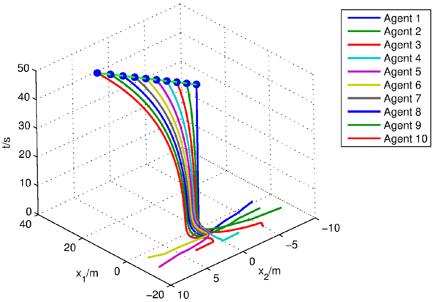
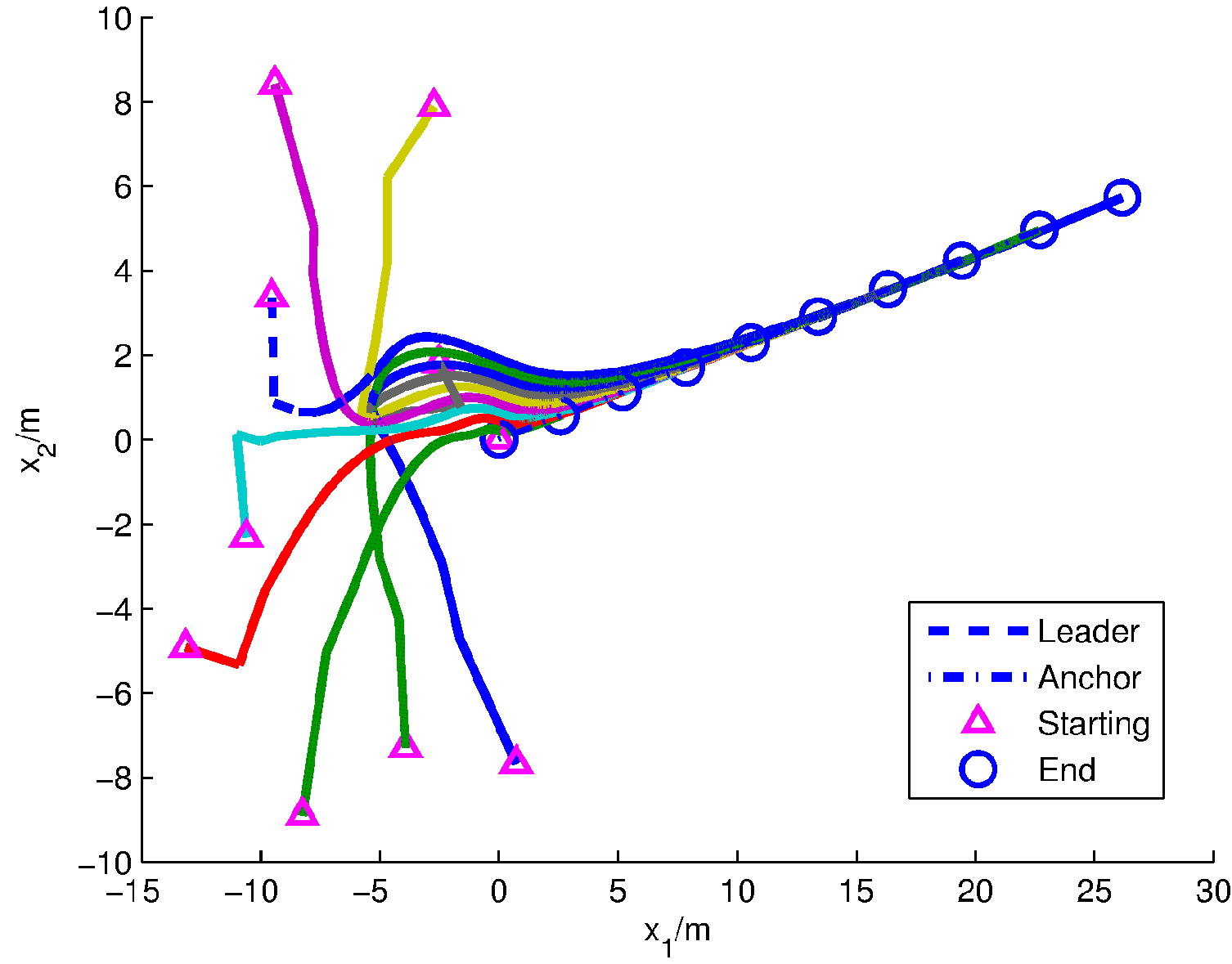
Our first scenario focuses on the mobile sensors in a straight line under the control law of the leader. The feedback gain of boundary controller is considered as follows: $K=\mathrm{diag}[5,8]$. Figure 1 depicts the spatio-temporal trajectories of the mobile sensors, which show that 10 agents move onto a desired straight line in the time interval $[0,40]$. Figure 1 is projected onto the plane $x_1{x}_2$ as Figure 2, where the motion of the mobile sensors on 2D can be clearly shown. The simulations above verify Theorem 2.

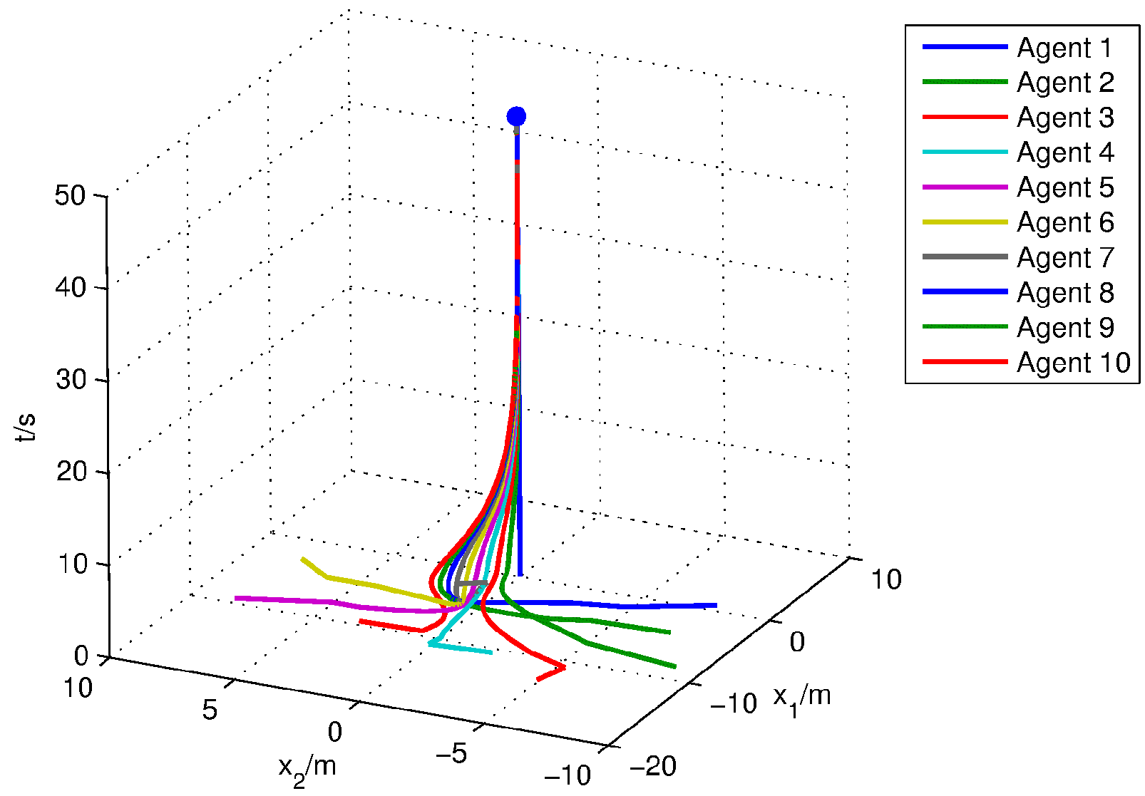
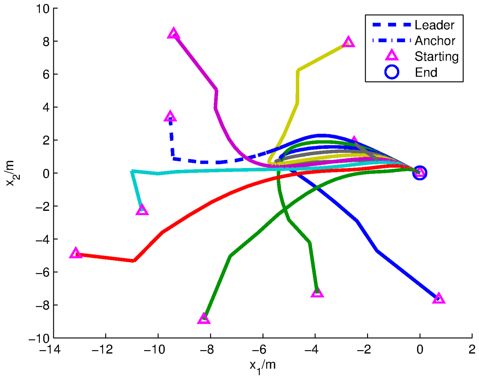
Next, Figure 3 is formed using parameter $K=\mathbf{0}$, which can verify Corollary 1. It is also clear that the distributed parameter multi-agent system under feedback input $v(\theta ,t)=\frac{{\partial }^{2}x(\theta ,t)}{\partial {\theta }^2}$ will rendezvous at the origin if no boundary controller is implemented by the leader. Figure 4 demonstrates the 2D trajectory of mobile sensors. As can be seen from it, 10 agents rendezvous at the origin on the projection plane $x_1{x}_2$.

6. Conclusions

This paper has studied the formation problem for an array of large mobile sensor networks. A new framework of mobile sensor networks has been introduced by modeling the dynamic of mobile sensors as a continuum which is described by the parabolic system with boundary disturbance such that the model of the system conforms more to the realities of the situation in nature. In this model, the communication topology of agents is a chain graph and fixed. By utilizing the Lyapunov functional method and boundary control approach, leader feedback laws which are designed in a manner for the boundary control of large mobile sensor networks allow the mobile sensors to stably achieve the formation. In fact, the large mobile sensor network addressed can be used for agricultural applications, the formation of unmanned aerial systems, and so on. Simulation results further illustrated the effectiveness of our results.

References

- Ma, Z.; Sun, Y.; Mei, T. A review of wireless sensor networks. J. Commun. 2004, 4, 114–124. [Google Scholar]
- Xu, Z.; Zhang, J. Analysis of wireless sensor network technology and its application technology bottleneck in Internet of Things. Internet Things Technol. 2011, 1, 79–81. [Google Scholar]
- Gharajeh, M.S.; Jond, H.B. An intelligent approach for autonomous mobile robots path planning based on adaptive neuro-fuzzy inference system. Ain Shams Eng. J. 2022, 13, 101491. [Google Scholar] [CrossRef]
- Chen, L.; Wang, Y.; Zhu, Q. Swarm formation control of multiple mobile robots based agent. Syst. Eng. Electron. 2006, 5, 731–735. [Google Scholar]
- Heidari, R.; Khajehzadeh, A.; Eslami, M. A consensus event-triggered control of networked multi-agent systems with non-ideal communication network. Ain Shams Eng. J. 2021, 12, 3783–3790. [Google Scholar] [CrossRef]
- Tu, Z.; Wang, Q.; Shen, Y. Simultaneous optimization of target tracking and monitoring in mobile sensor networks. J. Autom. 2012, 38, 452–461. [Google Scholar]
- Wu, M.; Li, L.; Wei, Z.; Wang, H. A consistent observation method for target tracking heterogeneous sensors in dynamic environment of mobile robots. J. Opt. 2015, 35, 202–210. [Google Scholar]
- Mao, W.; Zhang, W.; Qiu, X. Robot trajectory tracking control based on multi-sensor fusion. Control Eng. 2020, 27, 1125–1130. [Google Scholar]
- Liu, H.; Yang, H. Application of wireless sensing technology in building environment monitoring. Chem. Autom. Instrum. 2011, 38, 1413–1416. [Google Scholar]
- Sheng, X. A regional environmental monitoring system based on quadrotor UAVs. Internet Things Technol. 2021, 11, 25–26. [Google Scholar]
- Jia, S.; Gao, X.; Lu, Q. Distributed dynamic path planning algorithms in wireless sensor networks. J. Sens. Technol. 2013, 5, 695–700. [Google Scholar]
- Xiao, Q.; Ning, D. A swarming control model for mobile sensor networks based on tracking a single moving target. Comput. Knowl. Technol. 2014, 10, 1397–1400. [Google Scholar]
- Zhou, H.; Xu, C.; Li, D.; Shao, S. Application of cluster intelligence algorithm in WSN node localization. Comput. Eng. 2008, 20, 18–20. [Google Scholar]
- Fang, Z.; Gu, A.; Wang, L.; Zhang, X. Design of mobile robot system based on whisker sensor. China Instrum. 2009, 1, 82–84. [Google Scholar]
- Wang, J. Distributed target tracking based on sensing agents and movement control laws. J. Electron. Meas. Instrum. 2019, 33, 156–163. [Google Scholar]
- Zhong, L.; Lu, D.; Ye, J.; Qi, T. Distributed asynchronous measurement sensor network for robot control. Autom. Instrum. 2011, 26, 1–4. [Google Scholar]
- Deng, Y. Research on adaptive control of ship formation collision avoidance. Ship Sci. Technol. 2017, 39, 31–33. [Google Scholar]
- Wang, Y.; Hong, B. Fast convergence of distributed control algorithms for arbitrary formation of robot troops. Comput. Res. Dev. 2002, 10, 1274–1280. [Google Scholar]
- Li, J.; Peng, S.; An, H.; Xiang, X.; Shen, L. UAV formation aggregation method based on differential geometry and Lie group. J. NUDT 2013, 35, 157–164. [Google Scholar]
- Wu, Z.; Yu, H.; Wang, R. Flocking control of dynamic topology-based multiple motion agents with a leader. J. HUST (Nat. Sci. Ed.) 2008, 10, 29–31. [Google Scholar]
- Attanasi, A.; Cavagna, A.; Del Castello, L.; Giardina, I.; Grigera, T.S.; Jelić, A.; Melillo, S.; Parisi, L.; Pohl, O.; Shen, E.; et al. Information transfer and behavioural inertia in starling flocks. Nat. Phys. 2014, 10, 691–696. [Google Scholar] [CrossRef]
- Qin, W.; Zhuang, B.; Cui, B. Boundary control of crowd evacuation system based on continuum model. Control Decis. 2018, 33, 2073–2079. [Google Scholar]
- Qi, J.; Zhang, J. Boundary control for an unstable wave equation in annular with symmetrical initial data. J. DU (Eng. Ed.) 2016, 33, 467–472. [Google Scholar]
- Qi, J.; Wang, C.; Pan, F. Boundary observation and output feedback control for spherically symmetric n-dimensional reaction diffusion equations. J. Autom. 2015, 41, 1356–1364. [Google Scholar]
- Bao, L.; Huang, P. H∞ control of delayed distributed parameter switching systems. Sci. Technol. Eng. 2019, 19, 28–33. [Google Scholar]
- Qian, X. Global synchronization in an array of coupled neural networks with impulse and time-varying delayed coupling. J. YU (Nat. Sci. Ed.) 2011, 14, 21–26. [Google Scholar]
- Luo, S.; Chen, W. Periodic intermittent sampling control of a class of stochastic reaction diffusion neural networks. Syst. Sci. Math. 2017, 37, 652–664. [Google Scholar]
Disclaimer/Publisher’s Note: The statements, opinions and data contained in all publications are solely those of the individual author(s) and contributor(s) and not of MDPI and/or the editor(s). MDPI and/or the editor(s) disclaim responsibility for any injury to people or property resulting from any ideas, methods, instructions or products referred to in the content. |
© 2022 by the authors. Licensee MDPI, Basel, Switzerland. This article is an open access article distributed under the terms and conditions of the Creative Commons Attribution (CC BY) license (https://creativecommons.org/licenses/by/4.0/).