Tandem Recurrence Relations for Coefficients of Logarithmic Frobenius Series Solutions about Regular Singular Points

Abstract

We enhance Frobenius’ method for solving linear ordinary differential equations about regular singular points. Key to Frobenius’ approach is the exploration of the derivative with respect to a single parameter; this parameter is introduced through the powers of generalized power series. Extending this approach, we discover that tandem recurrence relations can be derived. These relations render coefficients for series occurring in logarithmic solutions. The method applies to the, practically important, exceptional cases in which the roots of the indicial equation are equal, or differ by a non-zero integer. We demonstrate the method on Bessel’s equation and derive previously unknown tandem recurrence relations for coefficients of solutions of the second kind, for Bessel equations of all integer and half-integer order.

1. Introduction

1.1. Subject, Problem, Main Goal and Results of This Manuscript

1.1.1. Main Subject of This Manuscript: Frobenius’ Method

In this manuscript, we significantly enhance Frobenius’ method for derivation of generalized power series solutions of linear ordinary differential equations with variable, analytical coefficients, about their regular singular points. As we shall explain, Frobenius’ method here refers to his method of exploring derivatives $d/dr$, with respect to a parameter r. This parameter r denotes the power of a prefactor to analytical series, as it occurs in generalized series solutions; the reader may want to have a look ahead, at Equations (5) and (8).

The standing problem, that hitherto has prohibited practical applications of Frobenius’ $d/dr$-method in important cases, but that we shall resolve in this paper, is identified in Section 1.1.2.

1.1.2. Current Status of Frobenius’ $d/dr$ Method and Problem Statement

The current, most practical, documented version of Frobenius’ $d/dr$-method can be found in references [1,2,3]. The method aims to calculate the coefficients $c_n$—see Equation (8)—of the correction series that may occur in generalized power series solutions. A crippling problem is that the current version of the method cannot be evaluated recursively.

Indeed, as we shall explain in detail in Section 4.3, when it comes to calculation of coefficient $c_n$, the documented methods [1,2,3] do not, and cannot, profit from the fact that at that stage the $c_m$ for $m<n$ are already known. Instead, the derivative $d/dr$ is to be applied to intermediate quantities $a_n\left(r\right)$ that have to be explicitly calculated as functions of parameter r and index n. This will usually have to be done explicitly for each subsequent integer value of n. Because these explicit expressions for the quantities $a_n\left(r\right)$ tend to be very complicated, and hence their subsequent derivations readily become enormously tedious, this strategy would render Frobenius’ $d/dr$-method virtually intractable in practical cases. This may explain that Frobenius’ $d/dr$ method, although its idea once was recommended ([4] (Section 3.5); [1] (Chapter V, VI)), is usually no longer covered in modern textbooks (see e.g., [5]).

1.1.3. Aim of This Manuscript

The aim of this manuscript is to develop Frobenius’ $d/dr$-method into a practical and efficient method and thus to reveal its full power. We focus on second order equations of which the indicial polynomial has only real roots. (The indicial polynomial and indicial equation are further introduced in Section 1.2.3 and Section 2.1.1. Of course, these concepts are also covered in the references [2,3]).

The novelty of our approach has bearing on the two so-called “exceptional cases” ([2], §4.6). The first of these concerns the second linearly independent solution in case the two roots of the indicial equation are equal. The second case concerns the solution associated with the smallest of the two roots, in case the two roots differ by a positive integer N.

1.1.4. Main Result

The key result presented in this manuscript is the existence of tandem recurrence relations for the coefficients of the second linearly independent solution of the differential equation, in the two exceptional cases just mentioned. We present a general method to construct these tandem recurrence relations. This renders our new, enhanced variant of Frobenius’ $d/dr$ method to be a practically applicable and rather efficient, algorithmic method for construction of generalized power series solutions, of Fuchsian differential equations, in all cases.

We shall be able to further specify our main result later, starting in Section 1.2.4.

1.1.5. Demonstration

So as to provide a non-trivial example, we demonstrate our method on Bessel’s equation, obtaining tandem recurrence relations for coefficients of solutions of the second kind, for Bessel equations of integer or half-integer order. (We follow the convention that a half-integer is a number of the form $n+\frac{1}{2}$, where n is an integer.) To our best knowledge, this particular representation of Bessel functions has not yet been documented in the literature.

1.2. Frobenius’ Method

1.2.1. Purpose of the Method; Regular Singular Points

Frobenius’ method [6] is widely established in textbooks [1,2,3,5,7,8,9,10] as a theory of solutions of linear ordinary differential equations

$$L\left[y\right(x),x]=0,$$

(1)

about their regular singular points. We will have explained how such points are characterized, and why the theory addressing them is invaluable, by the end of this subsection.

To avoid the prolixity that comes with unneeded generality, in this manuscript we shall restrict our presentation to cases of second order equations. Rephrased within the limitations of this restriction, Frobenius [6] opened his 1873 paper—see Figure 1—introducing the linear operator L (actually P in his notation) in our Equation (1) as

$$L[y\left(x\right),x]=x^2\lambda \left(x\right)y^{″}\left(x\right)+xp\left(x\right)y^{\prime }\left(x\right)+q\left(x\right)y\left(x\right).$$

(2)

Two restrictions are prescribed to the functions $\lambda \left(x\right)$, $p\left(x\right)$ and $q\left(x\right)$. Firstly, they must be analytical in a neighborhood of $x=0$, so they have series expansions

$$\lambda \left(x\right)=\sum _{n=0}^{\infty }{\lambda }_n{x}^n,p\left(x\right)=\sum _{n=0}^{\infty }{p}_n{x}^n,q\left(x\right)=\sum _{n=0}^{\infty }{q}_n{x}^n.$$

(3)

As a second restriction, we require that $\lambda \left(0\right)\ne 0$, or, equivalently,

$${\lambda }_0\ne 0.$$

(4)

These two restrictions together restrict $x=0$ to be what is now commonly known [2,3] as a regular singular point.

Note that the coefficient of the highest order derivative, $y^{″}\left(x\right)$ in (2), does vanish at the regular singular point $x=0$, because of the factor $x^2$. This makes $x=0$ a so-called singular point, at which the standard theorem for existence and uniqueness of solutions [2,3] for second order, linear differential equations does not apply. Points at which the coefficient of $y^{″}\left(x\right)$ does not vanish are called ordinary points. At such points the existence and uniqueness theorem for solutions is applicable.

From this context, it becomes clear that the theory of solutions about regular singular points is an extension of the standard theory of linear, ordinary differential equations: the theory is extended, so as to include at least a special class of singular points. Conditions (3) and (4) are such that the theory of Immanuel Lazarus Fuchs (1833–1902) [11,12] and Ferdinand Georg Frobenius (1848–1917) [6] applies, and they were indeed formulated by these founders of the theory. Their works have become invaluable for applied mathematics, because regular singular points are of vital importance in many applications in e.g., physics (see also, [13], e.g., and references therein).

The concepts and theory of regular singular points can, of course, be applied to other points $x=x_0$, by a simple change of variables $x\to x-x_0$ (see e.g., [3]).

1.2.2. Frobenius’ Ansatz and the Merits of His Approach

In his classic, seminal paper [6] on series solutions of differential equations, Frobenius revisited, and built on, the works of Fuchs [11,12]. (Both Fuchs and Frobenius were doctoral students of Karl Weierstrass, in Berlin.) and Thomé [14,15]. We shall pay due respect to Fuchs in Section 1.2.3.

Frobenius approach started from an Ansatz

$$y(x,r)=x^r\sum _{n=0}^{\infty }{a}_n{x}^n=\sum _{n=0}^{\infty }{a}_n{x}^{n+r},$$

(5)

through which parameter r is introduced. Frobenius’ original presentation of his Ansatz is shown in Figure 2.

Proceeding, Frobenius recovered, in a more direct and simpler [6,15] way, earlier results of Fuchs [11,12]. An overview was established of the solutions of (1) in the form of generalized power series (5) about the regular singular point $x=0$, possibly with an additional term involving a logarithmic factor. Frobenius [6] included a proof of uniform convergence of all series involved, concluding the proof that solutions of the differential equation had been achieved indeed [15].

One of the key merits of Frobenius’ approach and of his version of the theory, from a modern application point of view, is its directness and simplicity, as compared to the more indirect methods that Fuchs had applied. Frobenius’ approach readily provides a characterization of the solutions about regular singular points, in terms of whether or not their values are singular, whether or not their derivatives are singular and whether or not they have terms that include a logarithmic factor. Moreover, Frobenius’ method is constructive, in the sense that it renders algorithms for computation of solutions of differential equations. These algorithms indeed express the solutions in terms of no more than converging power series, logarithms and power functions. The radius of convergence of the series involved is also predicted by Frobenius’ theory.

1.2.3. On the Results of Fuchs

As said, Frobenius built on the works of Fuchs. Indeed, in the works of Fuchs the so called indicial equation

$$\rho \left(r\right)=0$$

(6)

for r can already be found; in this, for second order equations, the indicial polynomial $\rho \left(r\right)$ is defined as

$$\rho \left(r\right)={\lambda }_{0}r(r-1)+p_{0}r+q_0.$$

(7)

How the indidical polynomial and the indicial equation emerge from the theory, we shall indicate in Section 2, especially in Section 2.1.1.

The complete overview of the possible solutions of (1) associated with the roots of the indicial Equation (6) had also been established by Fuchs [11,12,15]. This included the result that, in cases in which the two roots $r_1$ and $r_2$ of the indicial equation differ by an integer N, i.e., $r_1-r_2=N$, a second independent solution $y_2\left(x\right)$ of (1), with (2), (3) and (5), is of the form

$$y_2\left(x\right)=ay(x,r_1)ln\left(x\right)+\sum _{n=0}^{\infty }{c}_n{x}^{n+r_2}.$$

(8)

N.B: At this stage, we allow N to be either equal to zero or to be a positive integer. Later in the manuscript the case $N=0$ needs to be distinguished. In this manuscript we shall restrict to cases in which the roots $r_1$ and $r_2$ of the indicial Equation (6) are real and we shall adhere to the convention that $r_1$ and $r_2$ are ordered as $r_2\le r_1$.

We add that the works of Fuchs actually covered n-th order linear differential equations, so that it provided generalizations of (8) to n-th order equations. But we shall not go into that here.

1.2.4. On What Frobenius Added to the Theory of Fuchs. Enhanced $d/dr$-Method

The novelty in Frobenius’ approach (i.e., his method) was the exploration of r, introduced through (5), as a parameter. This involved his derivation of especially the solutions of type (8), that possibly include logarithmic terms—coefficient a may vanish—by means of differentiation with respect to r; in what follows, we shall briefly refer to this as to the “$d/dr$-method”. As we shall explain further in Section 1.3, it is this method that we shall enhance in the present manuscript.

1.3. Tandem Recurrence Relations Emerging from the $d/dr$ Method

1.3.1. Relevance of Frobenius’ $d/dr$-Method and Our Enhancement of It

The $d/dr$ method is relevant to cases in which the roots of the indicial Equation (6) differ by an integer, including cases in which the roots are equal. A novel aspect that we shall present in the current manuscript is the fact that by the “$d/dr$-method” it is possible to derive a tandem of two interlinked recurrence relations. That is, two recurrence relations that combined allow for straightforward computation of the coefficients $c_n$ of (8).

The first member, (17), of the tandem, (17) combined with (18), is a recurrence relation for auxiliary coefficients $a_n\left(r_2\right)$ analogous to the $a_n$ in (5), but associated with the smallest root $r_2$ of the indicial equation. The second member of the tandem is recurrent in the $c_n$, but involves the $a_n\left(r_2\right)$. We shall also obtain the value of the coefficient a of the logarithmic term in (8).

1.3.2. Current Status of $d/dr$-Method and Novelty of Our Enhancement

Our technique to derive a tandem of recurrence relations for $c_n$ seems to not be widely known, if at all. The classic textbook by Boyce and DiPrima [3] does present formulae, partly without presenting the underlying theory, for the $d/dr$-approach in connection with solutions of type (8). How to apply these formulae is most explicitly outlined in Boyce and DiPrima’s [3] exercise about solving Bessel’s equation of order 1 by their version of the $d/dr$-method. This exercise truthfully follows Forsyth’s ([1], Chap. VI) solution of this problem, which was later recommended, but not covered in detail, by Watson ([4], Section 3.5). Earlier, Ince did include, in his extensive sections covering Frobenius’ method ([7], Section 16), a detailed presentation of Forsyth’s solution of Bessel’s equation ([7], Section 16.32), acknowledging Forsyth for it. Forsyth himself praised Frobenius’ process as being more general, simpler, and more direct ([1], Chap. VI), than the more conventional ways to introduce Bessel functions.

Yet, along the route that apparently Forsyth paved, to obtain the coefficients of generalized power series for Bessel functions of the second kind, it is required to solve the recurrence relation for the coefficients $a_n$, so as to obtain an explicit, non-recurrent expression for these. The tandem recurrence relations that we shall introduce are fully outside the scope of the Forsyth route. Indeed, as we shall discuss in Section 4.3, the formulae implementing the $d/dr$-method as presented in Boyce and DiPrima cannot be used to construct the tandem relations that we shall present. Actually, it seems that our tandem relations have not yet been documented at all in the existing literature.

1.3.3. Merit of Our Tandem Approach

The fact that solving a recurrence relation is no longer needed in our tandem approach greatly enhances the range and ease of application of the $d/dr$-method and indeed turns it into an algorithmic tool for solving Fuchsian differential equations. Furthermore, the existence of the tandem relations, and their structure, are of interest in their own right.

1.4. To Normalize or Not to Normalize the Coefficient of the Highest Order Derivative

1.4.1. Original Goal of the Theory

In his 1873 paper Frobenius merely set himself the task to recover, in a more direct and simpler way, results about the solutions of differential equations that Fuchs had published a decade earlier [11,12]. Given these aims, it is fully understandable that, to start with, Frobenius pointed out that the requirements put on $\lambda \left(x\right)$, $p\left(x\right)$ and $q\left(x\right)$ (in our notation here) allow for division by $\lambda \left(x\right)$. For a general theoretical treatment this is simply equivalent to assuming that $\lambda \left(x\right)=1$ and redefining $p\left(x\right)$ and $q\left(x\right)$. Therefore, “Zur Vereinfachung der Beweise” (“To simplify the proofs”; and see again Figure 2), Frobenius assumed $\lambda \left(x\right)=1$, indeed merely to simplify the notation throughout his paper.

1.4.2. The Normalization Convention in Textbooks

Textbooks [1,2,3,7,8,9,10] have followed this normalization convention ever since Frobenius. For theoretical purposes, no generality is lost. In applications however, $\lambda \left(x\right)$, $p\left(x\right)$ and $q\left(x\right)$ are often polynomials. In such cases, division by $\lambda \left(x\right)$ and redefining $p\left(x\right)$ and $q\left(x\right)$, such that the expansions (3) again apply, will turn $p\left(x\right)$ and $q\left(x\right)$ from finite degree polynomials into infinite series. The theoretical results of Frobenius are not sensitive to this. Indeed, his method is fully applicable to any analytical $p\left(x\right)$ and $q\left(x\right)$. Practically speaking however, division by $\lambda \left(x\right)$ may have both subtle and dramatic consequences, as outlined in the following paragraphs.

1.4.3. Why Normalization May Induce Complication

To further introduce this, we turn our attention to key ingredients in the theory, namely the recurrence relations for the coefficients $a_n$ of series (5). In the introduction of his 1873 paper Frobenius explicitly documented to have found (“fand ich”) that for solutions of differential equations as defined by (1) to (3), the coefficients of series solutions can be calculated quite simply (“einfach” and easily (“mit Leichtigkeit”); see also Figure 3). Apparently, by this he meant that, once the Ansatz (5) is accepted, deriving recurrence relations for the $a_n$ turns out to be straightforward. His subsequent proof of convergence, including the valuable proof that the radius of convergence is at least that of the series for $p\left(x\right)$ and $q\left(x\right)$, is founded on his method to calculate the coefficients.

In general, the recurrence relations for the $a_n$ tend to involve the previous coefficients $a_0,\dots ,a_{n-1}$, the number of which is strictly increasing as a function of n. That is, the recurrence relations for the $a_n$ tend to change in form and grow in size, as a function of n. Accordingly, the computations of the coefficients $c_n$ of solutions of type (8) will also increase in complexity as a function of n. The complexity of the computation of the coefficient a of the logarithmic term in (8) is affected likewise.

The coefficient a may vanish, and therefore its value is of considerable practical interest. As a criterion for this coefficient of the logarithmic term to vanish, Frobenius [6] recovered Fuchs’ [12] conditions, in terms of determinants of rows and columns representing the recurrence relations for the $a_n$. If the recurrence relations grow in length with increasing n, the complexity of the determinants increases accordingly, and as it concerns determinants, dramatically so.

These increases of complexities of the recurrence relations, and consequently of the determinants, with increasing value of index n, are induced only when any of the functions $\lambda \left(x\right)$, $p\left(x\right)$ and $q\left(x\right)$ needs to be represented by an infinite series.

1.4.4. Why Polynomial Coefficients Can Bring Computational Efficiency

When $\lambda \left(x\right)$, $p\left(x\right)$ and $q\left(x\right)$ all are polynomials however, of at most degree M, then for $M<n$, the recurrence relations for the coefficients $a_n$ of solutions of form (5) will at most depend on the M previous coefficients $a_{n-M},\dots ,a_{n-1}$. They will be functions of n, but, as we will highlight in the present manuscript, their computational complexity will no longer depend on n. In practice, they can actually simply be conceived as a single, fixed, closed form recurrence relation that depends on r, n and a fixed number of previous coefficients $a_m$, $m<n$. As we shall see, this simplicity carries over to the calculation of the coefficients $c_n$. As we indicated above, this simplicity may be lost, when $\lambda \left(x\right)$ is normalized to 1. Therefore, in Section 2, we shall avoid this normalization; this in itself evokes a slight generalization of Frobenius original formulae [6].

1.5. Outline

The plan for this manuscript further is as follows.

1.5.1. Exposition of the Theory

In Section 2, we shall revisit, and further develop understanding of, Frobenius’ approach to the solutions of linear second order differential equations as specified by relations (1) to (3). The first of our results consists of the combination of expressions (17) and (18). These relations form a tandem of two recurrence relations. From it, the coefficients of an, as such well-known [2,3], series solution containing a logarithmic term, (20), can be obtained. In Section 2.2.5 we show that and how relation (18) can be derived by differentiation with respect to Frobenius’ parameter r.

In Section 2.2.5 we obtain this result for the case of two equal roots of the indicial equation. In Section 2.3 we obtain a similar result for the more subtle case in which the two roots differ by a non-zero integer N, $r_1-r_2=N$.

An important difference between the two cases is that, while for equal roots, i.e., if $r_1=r_2$, a logarithmic term always occurs in the second independent solution of the differential equation, in cases $r_1-r_2=N$ the logarithmic term may vanish. As we shall discuss in Section 2.3.8, solutions of a differential equation about so-called ordinary points turn out to be an example of this. Another important example is provided by Bessel functions of second kind and half-integer order, to be covered in appropriate detail in Section 3.5.3.

1.5.2. Demonstration: Bessel’s Equation

We shall solve Bessel’s equation with our enhanced version of Frobenius’ method so as to provides illustrative and useful examples of tandem recurrence relations for series solutions. We derive such relations relevant to Bessel functions of the second kind in the course of Section 3; these tandem recurrence relations do not seem to have been documented yet in the literature.

1.5.3. Summary, Reflection and History

Section 4 provides a summary of the main results and a concise reflection on the history of key ingredients of the material. The reason for postponing this reflection to Section 4, instead of incorporating it in this introductory Section 1, is that we feel that a comprehensible reflection on these matters is really only possible after the theory in Section 2 and Section 3 has been presented.

The historical reflection in Section 4 is essentially an attempt to understand why the full power of the $d/dr$-method has only come to surface now, i.e., almost one and a half century after Frobenius first introduced the approach of exploring $d/dr$.

2. Analysis and Enhancement of Frobenius’ Method

2.1. Frobenius’ Expansion of the Image of the Differential Operator, First Solution of the Differential Equation and Second Solution When the Roots of the Indicial Equation Are Unequal and Do Not Differ by an Integer

2.1.1. General Expansion of the Image of the Differential Operator

As we mentioned in the Introduction, Frobenius’ approach to construct solutions for Equation (1), (2) builds on the Ansatz (5). The existence and details of a first solution $y_1$ of this form readily follow from substitution of (3) and (5) into (2) and expanding. As a first and founding step of his approach however, Frobenius’ wrote down the result of such an expansion for general r. Following this initiative, we arrive at the following expansion of the image of any function $y(x,r)$ of the form (5), as produced by the differential operator (2), with $\rho \left(r\right)$ as in (7),

$$\begin{array}{c}L[y(x,r),x]=\rho \left(r\right)a_0{x}^r+\hfill \\ \hspace{1em}\sum _{n=1}^{\infty }\left(\rho (n+r)a_n+\sum _{i=0}^{n-1}\left((i+r)(i+r-1){\lambda }_{n-i}+(i+r)p_{n-i}+q_{n-i}\right)a_i\right)x^{n+r};\hfill \end{array}$$

(9)

We emphasize that this expansion is valid for any value of r.

2.1.2. Solution Associated with the Largest Root of the Indicial Equation

From (9), it follows that $y(x,r_1)$, in which $r_1$ is the largest root of the indicial Equation (6), so that $\rho \left(r_1\right)=0$, and with $y(x,r)$ as given by (5), provides a first solution of (1) if its coefficients $a_n$ satisfy

$$\begin{array}{c}\rho (n+r_1)a_n+\hfill \\ \hspace{1em}\hspace{1em}+\sum _{i=0}^{n-1}\left((i+r_1)(i+r_1-1){\lambda }_{n-i}+(i+r_1)p_{n-i}+q_{n-i}\right)a_i=0,1\le n.\hfill \end{array}$$

(10)

Since $r_1$ is the largest of the roots $r_1$ and $r_2$ of the indicial equation $\rho \left(r\right)=0$, it follows that $\rho (n+r_1)\ne 0$, for all n, $1\le n$. Relation (10) then provides a recurrence relation, which uniquely defines the values of all of the coefficients $a_n$, given $r_1$ and any chosen value for $a_0$.

2.1.3. Second Linearly Independent Solution? Emergence of the So-Called Exceptional Cases

A second independent solution $y_2(x,r_2)$ of (1) of the form (5) exists, fully analogous to $y(x,r_1)$, if $r_1\ne r_2$ and provided $\rho (n+r_2)\ne 0$, for all n, $1\le n$. The second condition is equivalent to $r_1-r_2$ not being equal to a positive integer.

Frobenius’ method [6] is especially distinguished when these latter conditions are violated, i.e., when either $r_1=r_2$ or $r_1-r_2=N$, in which N is a positive integer. These cases have been referred to as to the exceptional cases ([2], §4.6), but precisely these have turned out to frequently be of great relevance in mathematical physics ([9], §3.5), [13].

2.2. Conception of the $d/dr$ Method, General Relations Central to the Method and Second Linearly Independent Solution in Case the Roots of the Indicial Equation Are Equal

2.2.1. Inspiration from the Case in Which the Roots of the Indicial Equation Are Equal

In case the two roots $r_1$ and $r_2$ of the indicial equation $\rho \left(r\right)=0$, (6), are equal, the graph of $\rho \left(r\right)$ will be a parabola tangent to the horizontal axis of the $(r,\rho )$ plane. In that case, together with its value $\rho \left(r_1\right)=\rho \left(r_2\right)=0$, the derivative ${\rho }^{\prime }\left(r\right)$ of the function $\rho \left(r\right)$ will also vanish for $r=r_1$; i.e., we shall have both$\rho \left(r_1\right)=0$ and ${\rho }^{\prime }\left(r_1\right)=0$. In view of the fact that $\rho \left(r\right)$ appears in the leading term at the right hand side of expression (9), this coincidence can be taken as a hint to explore the derivatives of both sides of expression (9) with respect to r.

A step that will enable us to actually focus on the first term at the right hand side of expression (9), is to introduce, and confine ourselves to, a class of functions, such that the nested sum in expression (9) will vanish identically.

2.2.2. Frobenius’ Class of Functions $\tilde{y}(x,r)$ and General Relations Central to the $d/dr$ Method

The right hand side of expression (9) can be simplified significantly, if, following an initiative that Frobenius took on the fourth page of his 1873 paper, we introduce the notation $\tilde{y}(x,r)$ for functions $y(x,r)$ of the form (5) while their coefficients $a_n$ furthermore are required to satisfy

$$\rho (n+r)a_n+\sum _{i=0}^{n-1}\left((i+r)(i+r-1){\lambda }_{n-i}+(i+r)p_{n-i}+q_{n-i}\right)a_i=0,1\le n;$$

(11)

this relation indeed ensures that the nested sum in expression (9) will vanish identically, whenever $y(x,r)$ is of the type $\tilde{y}(x,r)$.

Note that satisfying (11) would not be hindered by occurrence of $\rho (n+r_2)=0$ for some value N of n (as may happen when $N=r_1-r_2$, for some positive integer N). Such occurrence would possibly prevent (11) to have a unique solution for the $a_n$, $1\le n$, but it would not prevent it to have a solution at all.

Also note that, again following Frobenius, we explicitly do not yet require r to be a solution of the indicial equation; rather, r is explicitly kept as a parameter of the functions $\tilde{y}(x,r)$. Note furthermore that relation (11) then implies that the coefficients $a_n$ will be functions of r. Once more following Frobenius, we now also explicitly allow $a_0$ to depend on r. As we shall discuss in Section 4, the possible dependence of $a_0$ on r does turn out to play a key role in the theory, be it seemingly in a different way than originally anticipated by Frobenius.

The key advantage of the introduction of the functions $\tilde{y}(x,r)$ is that, when expression (9) is applied to this class of functions, the nested series on the right hand side of (9) will vanish regardless the value of r, and hence so will its derivative with respect to r. Hence, provided it is allowed to interchange the order of derivatives with respect to x and r respectively, taking the derivative with respect to r of the both sides of expression (9) leads to

$$L[\frac{d\tilde{y}(x,r)}{dr},x]=\left(\left(\frac{d{a}_0\left(r\right)}{dr}+a_0\left(r\right)ln\left(x\right)\right)\rho \left(r\right)+a_0\left(r\right)\frac{d\rho \left(r\right)}{dr}\right)x^r.$$

(12)

2.2.3. First Application of the $d/dr$ Method: Solutions in Case the Roots $r_1$ and $r_2$ of the Indicial Equation Are Equal

From relation (12) it follows that in case $r_1=r_2$ we shall have

$$L[\frac{d\tilde{y}(x,r)}{dr},x]{|}_{r=r_1}=0,$$

since, as we discussed, $r_1=r_2$ implies that together with $\rho \left(r_1\right)=0$ we shall have ${\rho }^{\prime }\left(r_1\right)=0$. Hence the function

$$\frac{d\tilde{y}(x,r)}{dr}=\sum _{n=0}^{\infty }\frac{d{a}_n\left(r\right)}{dr}{x}^{n+r}+ln\left(x\right)\sum _{n=0}^{\infty }{a}_n\left(r\right)x^{n+r},$$

(13)

provided all series involved converge, after substitution $r=r_1$ reduces to a second solution

$$\begin{array}{cc}\hfill y_2\left(x\right)& =\frac{d\tilde{y}(x,r)}{dr}{|}_{r=r_1}\hfill \\ \hfill & =\sum _{n=0}^{\infty }\frac{d{a}_n\left(r\right)}{dr}{|}_{r=r_1}{x}^{n+r_1}+ln\left(x\right)\sum _{n=0}^{\infty }{a}_n\left(r_1\right)x^{n+r_1},(r_1=r_2),\hfill \end{array}$$

(14)

of the differential Equation (1) in the exceptional case of equal roots of the indicial equation. Given the occurrence of the singular factor $ln\left(x\right)$, it is straightforward to show that $y_2\left(x\right)$ (14) and $y(x,r_1)$ will be linearly independent.

2.2.4. The Derivative of the First Recurrence Relation with Respect to Frobenius’ Parameter r

An aspect that, to the best of the author’s knowledge, has not yet been mentioned in the existing literature as yet, is the following. Relation (11) is considered to be an identity in r. From this it follows that the derivative of the left hand side of relation (11) with respect to r must identically vanish. Consequently,

$$\begin{array}{c}\hfill \rho (n+r)\frac{d{a}_n\left(r\right)}{dr}+\sum _{i=0}^{n-1}\left((i+r)(i+r-1){\lambda }_{n-i}+(i+r)p_{n-i}+q_{n-i}\right)\frac{d{a}_i\left(r\right)}{dr}+\\ \hfill +{\rho }^{\prime }(n+r)a_n+\sum _{i=0}^{n-1}\left((2(i+r)-1){\lambda }_{n-i}+p_{n-i}\right)a_i=0,1\le n.\end{array}$$

(15)

In this, ${\rho }^{\prime }\left(r\right)$ denotes the derivative of the indicial polynomial function (7).

We emphasize here that relation (15) is valid for any r. We shall now first apply it in the case $r_1=r_2$. In Section 2.3 we shall apply it to the other exceptional case, i.e., when $r_1-r_2=N$, in which N then will be a positive integer.

2.2.5. Tandem Recurrence Relations for Generalized Power Series Coefficients in Case $r_1=r_2$

In the case of equal roots of the indicial equation, $r_1=r_2$, relation (15), together with relation (11) itself, will form a tandem of recurrence relations for the coefficients $a_n$ and $b_n$, with

$$b_n=\frac{d{a}_n\left(r\right)}{dr}{|}_{r=r_1},$$

(16)

occurring in solution (14). Indeed, relation (11), with $r_1$ substituted for r, forms the first member of this tandem:

$$\begin{array}{cc}\hfill & \rho (n+r_1)a_n\left(r_1\right)+\hfill \\ \hfill & +\sum _{i=0}^{n-1}\left((i+r_1)(i+r_1-1){\lambda }_{n-i}+(i+r_1)p_{n-i}+q_{n-i}\right)a_i\left(r_1\right)=0,1\le n.\hfill \end{array}$$

(17)

From this recurrence relation the coefficients $a_n\left(r_1\right)$ follow, given any choice of $a_0\left(r_1\right)$. The second member of the tandem follows from relation (15), using (16) and after substitution of $r_1$ for r:

$$\begin{array}{cc}\hfill & \rho (n+r_1)b_n+\sum _{i=0}^{n-1}\left((i+r_1)(i+r_1-1){\lambda }_{n-i}+(i+r_1)p_{n-i}+q_{n-i}\right)b_i+\hfill \\ \hfill & +{\rho }^{\prime }(n+r_1)a_n\left(r_1\right)+\sum _{i=0}^{n-1}\left((2(i+r_1)-1){\lambda }_{n-i}+p_{n-i}\right)a_i\left(r_1\right)=0,1\le n.\hfill \end{array}$$

(18)

This relation provides a recurrence relation for the coefficients $b_n$, (16). Because, in case $r=r_1=r_2$, for $1\le n$ the coefficient $\rho (n+r_1)$ of $b_n$ will not vanish, the recurrence relations (18) uniquely define the values of the coefficients $b_n$, for all $1\le n$. Note that (18) takes the $a_n\left(r_1\right)$, as calculated from relation (17) as input. It is in this sense that (17) and (18) form a tandem.

The coefficients $a_m\left(r_1\right)$ in (18) were defined by recurrence relation (11) with $r=r_1$, i.e., by (17) actually, for any choice of $a_0\left(r\right)$. Using the conventional choice $a_0\left(r_1\right)=1$, and reusing this for the second solution, the $a_n\left(r_1\right)$ are really the same coefficients as those of the solution $y(x,r_1)$. With this choice, according to (16),

$$b_0={\left(\frac{d{a}_0\left(r\right)}{dr}\right)}_{|r=r_1}=0,$$

(19)

so that in case $r_1=r_2$, from (14) we recover the well-known [2,3,9] result that

$$y_2\left(x\right)=ln\left(x\right)y(x,r_1)+\sum _{n=1}^{\infty }{b}_n{x}^{n+r_1}$$

(20)

provides a second linearly independent solution of the differential equation.

2.2.6. The Novelty of, and Enhancement Established by, the Tandem Technique

The novelty rendered by our reconstruction of (20), i.e., our enhancement of the underlying $d/dr$-method, lies in the fact that the coefficients $b_n$ can be computed, algorithmically, from the tandem formed by relations (17) and (18), starting from $a_0=1$ and $b_0=0$. The decisive enhancement established by our tandem method lies in the fact that it eliminates the need to solve the recurrence relations (11) for the $a_n\left(r\right)$, so as to obtain all the coefficients $a_n\left(r\right)$ explicitly as functions of r. (Relation (16) seems to have been interpreted, mistakenly, as to suggest such a need; indeed Boyce and DiPrima [3], in their discussion of application of relation (16), mentioned the need to “first determine $a_n\left(r\right)$′).

Indeed, solving recurrence relations (11) for the $a_n$ as explicit functions of r can be forbiddingly complicated, or even difficult, whereas recursive evaluation of our tandem (17) and (18) is merely a routine, in all cases. As a result, once enhanced with our tandem technique, Frobenius’ $d/dr$-method becomes an efficient, algorithmic method for routinely solving differential equations about their regular singular points.

2.3. Solutions Associated with $r_2$ in Case $r_1-r_2=N$

2.3.1. Structure of Indicial Polynomial

Because $r_1$ and $r_2$ are the roots of the indicial polynomial $\rho \left(r\right)$, we can rewrite $\rho \left(r\right)$ (7) as

$$\rho \left(r\right)={\lambda }_0(r-r_1)(r-r_2).$$

(21)

Hence, the pre-factor of $a_N$ according to (11) for $n=N$, which is the same as that of $d{a}_N/dr$ according to (15) for $n=N$, is

$$\rho (N+r)={\lambda }_0(r-(r_1-N))(r-(r_2-N)).$$

(22)

In case the two roots $r_1$ and $r_2$, of the indicial polynomial differ by a positive integer number N, $r_1-r_2=N$, expression (22) reduces to

$$\rho (N+r)={\lambda }_0(r-r_2)(r-(r_2-N)),\mathrm{in} \mathrm{case} r_1-r_2=N.$$

(23)

Hence, in case $r_1-r_2=N$, in which N is a positive integer, the pre-factor of $a_N$ according to (11) and that of $d{a}_N/dr$ according to (15), vanishes if $r=r_2$. Hence, the coefficient $a_N$ and the quantity $d{a}_N/dr$ remain free, as far as Equations (11) and (15) are concerned. With respect to possible solutions $y(x,r_2)$ of the form (5), i.e., without logarithm, with $r=r_2$ and with the coefficients obeying (11), the situation is then as outlined in the next subsection.

2.3.2. With $r=r_2$ and the Free Coefficient $a_N$, a Solution Linearly Dependent on $y(x,r_1)$ Is Associated

Since the coefficient of $a_N$ vanishes for $r=r_2$, Equation (11) for $n=N$ reduces to a relation for $a_0,a_1,\dots ,a_{N-1}$. This implies that for $n=1,\dots ,N$, Equation (11) provides a homogeneous system of N coupled linear algebraic equations for the N coefficients $a_0,a_1,\dots ,a_{N-1}$. The matrix of coefficients of this system may be singular, in which case the system would allow for a non-trivial solution.

We insert two remarks, labeled for later reference:

Remark 1.

From the recurrent structure of the equations, combined with the fact that the coefficient of $a_n$ in Equation (11) will be non-zero for $n=1,\dots ,N-1$, it is clear that any non-trivial solution for coefficients $a_0,a_1,\dots ,a_{N-1}$ would have at most a single free parameter: all coefficients $a_1,\dots ,a_{N-1}$ could be expressed as functions of $a_0$.

Remark 2.

In any case, the system of N coupled linear algebraic equations will have the trivial solution

$$a_0=0,\dots ,a_{N-1}=0.$$

We shall refer back to the case of non-trivial solutions, Remark 1, later. We shall now first further explore the trivial solution $a_0=0,\dots ,a_{N-1}=0$, Remark 2.

Proceeding—regardless of the matrix being singular or non-singular—with the trivial solution $a_0=0,\dots ,a_{N-1}=0$, combined with free coefficient $a_N$, expression (11) provides recurrence relations for all $a_m$, $N+1\le m$. In this way it does provide a solution $y(x,r_2)$ of the form (5), with $r=r_2$. Rewriting (11), for $N\le n$, in terms of new indices of summation $m=n-N$ and $j=i-N$, using $r_1-r_2=N$, and finally expressing the result in terms of new coefficients $d_m=a_{m+N}$ reveals that the solution $y(x,r_2)$ thus obtained is the same as, or a multiple of, $y(x,r_1)$.

In summary, if $r_1-r_2=N$, for any positive integer N, then through its solution initiated by $a_0=0,\dots ,a_{N-1}=0$ and its free parameter $a_N$, when applied to construct solutions of the form (5) with $r=r_2$, relation (11) renders a solution that is merely a multiple of $y(x,r_1)$.

2.3.3. Second Linearly Independent Solution in Case $r_1-r_2=N$

In this subsection we continue to explore Remark 2: we continue to explore the trivial solution

$$a_0=0,\dots ,a_{N-1}=0,$$

(24)

of the set of algebraic equations that is obtained from (11) for $n=1,\dots ,N$. In case $r_1-r_2=N$, an independent second solution of differential Equation (1) is associated with the smallest root $r=r_2$ of the indicial equation, combined with the trivial solution $a_0=0,\dots ,a_{N-1}=0$, as follows.

Obviously, since $r_2$ is a root of the indicial Equation (6), we have $\rho \left(r_2\right)=0$. Hence, since we have $a_0=0$, when $r=r_2$ is substituted into expression (12), the right hand side of expression (12) will vanish. This just shows that expression (13) will reduce to a solution of differential Equation (1) if we substitute $r=r_2$ into it, while we have $a_0=0$. This solution takes the form

$$y_2\left(x\right)=\sum _{n=0}^{\infty }{c}_n{x}^{n+r_2}+ln\left(x\right)\sum _{n=0}^{\infty }{a}_n\left(r_2\right)x^{n+r_2}.$$

(25)

With $a_0\left(r_2\right)=0,\dots ,a_{N-1}\left(r_2\right)=0$ and the coefficients $a_n\left(r_2\right)$ satisfying (11), we identify the second series as $a_N\left(r_2\right)y(x,r_1)$, so we recover the familiar result [1,2,3,7]

$$y_2\left(x\right)=\sum _{n=0}^{\infty }{c}_n{x}^{n+r_2}+a_N\left(r_2\right)ln\left(x\right)y(x,r_1).$$

(26)

2.3.4. Tandem Recurrence Relations for the Coefficients $c_n$

The coefficients $c_n$ in (25) or (26), defined fully analogously to (16), as

$$c_n=\left(\frac{d{a}_n\left(r\right)}{dr}\right){|}_{r=r_2},$$

(27)

must furthermore satisfy relation (15) for $r=r_2$, so

$$\begin{array}{cc}\hfill & \rho (n+r_2)c_n+\sum _{i=0}^{n-1}\left((i+r_2)(i+r_2-1){\lambda }_{n-i}+(i+r_2)p_{n-i}+q_{n-i}\right)c_i+\hfill \\ \hfill & +{\rho }^{\prime }(n+r_2)a_n\left(r_2\right)+\sum _{i=0}^{n-1}\left((2(i+r_2)-1){\lambda }_{n-i}+p_{n-i}\right)a_i\left(r_2\right)=0,1\le n;\hfill \end{array}$$

(28)

the coefficients $a_m\left(r_2\right)$ in this are the solutions of relation (11), for $r=r_2$ and with starting values (24).

So, the tandem of recurrence relations for the $c_n$ consists of relation (28), and relation (11), for $r=r_2$ and with starting value $a_0=0$. The coefficient $c_0$ remains a free, and can be viewed as a free constant of integration. NB: in Section 2.3.6, we shall consider $a_N\left(r_2\right)$, which is the important coefficient of the logarithmic factor in (20).

2.3.5. Why $c_N$ Remains a Free Parameter and the Meaning of this

In the context of relation (28) with $n=N$, it is now $c_N$ which appears as a free, undetermined coefficient. In view of $r=r_2$, the form of the series in which $c_N$ appears and in the light of our discussion above of how a free $a_N\left(r_2\right)$ in the context of (5) merely produces a copy of $y(x,r_1)$, we recognize that the free coefficient $c_N$ once more represents the possibility to add a multiple of $y(x,r_1)$ to (25).

2.3.6. How to Obtain $a_N\left(r_2\right)$, the Coefficient of the Logarithmic Factor

Note furthermore that in the new context of (25) and (28), the coefficient $a_N\left(r_2\right)$ is no longer free: its coefficient in relations (28), for $n=N$, does not vanish. Indeed, this coefficient is ${\rho }^{\prime }(N+r_2)={\rho }^{\prime }\left(r_1\right)$, and since $r_1\ne r_2$, certainly ${\rho }^{\prime }\left(r_1\right)\ne 0$. Hence, given $a_0\left(r_2\right)=0,\dots ,a_{N-1}\left(r_2\right)=0$, the coefficient $a_N\left(r_2\right)$ is actually determined by the recurrence relation for the $c_n$, (28), for $n=N$, i.e., by

$${\rho }^{\prime }\left(r_1\right)a_N\left(r_2\right)+\sum _{i=0}^{N-1}\left((i+r_2)(i+r_2-1){\lambda }_{N-i}+(i+r_2)p_{N-i}+q_{N-i}\right)c_i=0.$$

(29)

The $c_i$ occurring in this equation are to be obtained from relations (28) for $n=1,\dots ,N-1$, i.e., from

$$\begin{array}{cc}\hfill \rho (n+r_2)c_n+\sum _{i=0}^{n-1}\left((i+r_2)(i+r_2-1){\lambda }_{n-i}+(i+r_2)p_{n-i}+q_{n-i}\right)c_i& =0,\hfill \\ \hfill 1\le n& \le N-1,\hfill \end{array}$$

(30)

so that, as mentioned, $c_0$ is left as a free coefficient; this represents the scaling freedom of solution $y_2\left(x\right)$, due to the linearity of the differential equation.

2.3.7. Intermediate Summary of the Method for Case $r_1-r_2=N$

Summarizing the results of Section 2.3.3, Section 2.3.4, Section 2.3.5, Section 2.3.6, we can state that the values of the $c_n$ are rendered by their recurrence relation (28), except $c_N$, which remains free. For $n=N$, instead of $c_N$, relation (28) renders $a_N\left(r_2\right)$, the coefficient of the logarithmic term in the solution $y_2$, (26).

The coefficients $a_n\left(r_2\right)$ are rendered by recurrence relation (11), with starting value $a_0=0$. However, note that for $n=N$, relation (11) does not determine $a_N\left(r_2\right)$. For $N<n$ recurrence relation (11) again renders the values of the $a_n\left(r_2\right)$, taking $a_N\left(r_2\right)$ (which was determined by (28), as just explained) as an input.

The freedom of $c_N$ corresponds to the fact that a scalar multiple of $y_1$ may always be added to $y_2$, thanks to the linearity of the differential equation. The coefficient $c_0$ remains free as a constant of integration.

2.3.8. Possibility of Solutions Associated with $r_2$ without a Logarithmic Term

We recall that in the previous subsections, we are aiming to construct a solution of type (26). The procedure is to calculate coefficients $a_n\left(r_2\right)$ and $c_n$ using the tandem of recurrence relations (11) and (28), starting from $a_0\left(r_2\right)=0,\dots ,a_{N-1}\left(r_2\right)=0$ and having $c_0$ as a non-zero, free coefficient. As a special case of (28), namely for $n=N$, we have relation (29), which determines $a_N\left(r_2\right)$.

Depending on the values of the coefficients ${\lambda }_j$, $p_j$ and $q_j$ then, it may occur that (29) implies that $a_N\left(r_2\right)$ vanishes, too. The logarithmic term in solution of type (26) then would vanish, i.e., in these cases we find a second solution of type (5), with $r=r_2$, without logarithmic term.

In such cases, it would furthermore follow from (11) that all $a_n\left(r_2\right)$ vanish. An immediate consequence of this is that relation (28) for the coefficients $c_i$ will essentially reduce to what relation (11) is for the coefficients $a_i\left(r_2\right)$.

In other words, in these cases it would have been possible to find these same solutions of type (26) with vanishing logarithmic term, i.e., of type (5), associated with $r_2$, directly from (11). Recalling that $c_0$ is non-zero, this means that the corresponding solution of (11), with $r=r_2$, has non-zero $a_0$. Hence this situation corresponds precisely to a possible non-trivial solution of (11) with $r=r_2$ (which, as we saw, has at most a single free parameter, e.g., $a_0$) as meant in Remark 1.

(Note: this case neatly corresponds to a heuristic recommended by Boyce and DiPrima [3]: in case $r_1$ and $r_2$ differ by a positive integer, one may still attempt to find a second linearly independent solution of type (5) using recurrence relation (11) with $r=r_2$. Only if such an attempt is unsuccessful, one needs to proceed looking for a solution of form (26)).

Note furthermore that the solution $y(x,r_2)$ associated with $r_2$ thus found is linearly independent of $y(x,r_1)$. This easily follows from the observation that the lowest powers of x occurring in the two solutions are precisely $r_2$ and $r_1$ respectively, and these powers differ, by N.

A unifying example of this case occurs when a differential equation, for which $x=0$ is an ordinary point—see Section 1.2.1—is multiplied by $x^2$. When the resulting equation, for which $x=0$ is treated as a regular singular point, then is solved about $x=0$ by the method discussed in this section, one finds $r_1=1$ and $r_2=0$. The logarithmic term of the second independent solution, associated with $r_2=0$, can subsequently be easily shown to always vanish.

A less trivial example is provided by Bessel equations of half-integer order, to be addressed in detail as an example application in Section 3.5.3. About a feature of Bessel functions that is relevant to our study here, Watson ([4], Section 3.11) remarked in his Treatise:

“(…) no modification in the definition of $J_{\nu }\left(z\right)$ is necessary when $\nu$ (is half-integer); the real peculiarity of the solution in this case is that the negative root of the indicial equation gives rise to a series containing two arbitrary constants, i.e., to the general solution of the differential equation.”

As we revealed in the present section, this peculiarity of the Bessel functions of second kind and half-integer order is an instance of a more general phenomenon.

2.3.9. Conclusions

The major new result achieved in Section 2.3 lies in the fact that the combination of relations (28) and (11), for $r=r_2$, forms a tandem of interlinked recurrence relations, that as a whole renders the coefficients $c_n$ of the solution (26). They are to be used with the condition $a_0\left(r_2\right)=0$, while $c_0$ is to be a free, but non-zero parameter of the final solution; it is actually a free constant of integration, reflecting linearity of the differential Equation (1).

Our formulation (28) reveals that, in case the second independent solution does have a non-vanishing logarithmic term, the recurrence relations determining the $c_n$ change drastically at $n=N$: for $n<N$, all $a_n$ vanish, while for $N\le n$ they typically do not. Nota bene: this explains why it is considered to be “usually impossible” ([5], §9.5) to find closed form expressions for the coefficients $c_n$, i.e., to have the coefficients $c_n$ as explicit functions of n.

Relations (28) and (11) also show that, when $\lambda \left(x\right)$, $p\left(x\right)$ and $q\left(x\right)$ are all finite degree polynomials, say of degree K, then for $K\le n$ the sum over $i=0,\dots ,n-1$ reduces to a sum $i=n-K,\dots ,n-1$. That is, the number of terms generated by this sum then becomes constant and equal to at most K, and it is no longer increasing with n. Relations (28) and (11) then become closed form recurrence relations: they will be functions of n, and of the coefficients of the polynomials $\lambda \left(x\right)$, $p\left(x\right)$ and $q\left(x\right)$, but they will be the same in form (i.e., form invariant) for all $a_n$ and $c_n$, $K\le n$. This advantage may be lost when the differential Equation (1) is divided by $\lambda \left(x\right)$, so as to normalize the coefficient of $y^{″}$ and it is for this reason that we avoided this normalization in our assessment of the subject.

3. Application: Series Solutions for Bessel’s Equation

To highlight the novelty in our results, by way of an example, we shall apply essentially relations (11), (18) and (28) to construct form invariant recurrence relations for coefficients of all solutions of Bessel’s equation, for all positive real order $\nu$. Especially the tandem recurrence relations for the coefficients $a_n$, $b_n$ and $c_n$ that we shall derive for solutions of Bessel’s equation of integer or half-integer order, as far as the author has been able to verify, have not previously been documented in the literature.

Note: We follow terminology that is common in the literature about Bessel functions: in this context, the order of a Bessel equation is understood to refer to the value of the parameter $\nu$, not to the highest order of the derivatives that occur in the equation. The order of a Bessel equation thus corresponds to the index of the Bessel functions that are its solutions.

3.1. Coefficients and Indicial Polynomial

Bessel’s equation of order $\nu$

$$x^2{y}^{″}\left(x\right)+x{y}^{\prime }+(x^2-{\nu }^2)y=0,$$

(31)

clearly is of form (1)–(3). The only non-zero coefficients of its series (3) are

$${\lambda }_0=1,p_0=1,q_0=-{\nu }^{2}and{q}_2=1,$$

(32)

so that the roots $r_1$ and $r_2$ of the associated indicial polynomial (7)

$$\rho \left(r\right)=r^2-{\nu }^2,$$

(33)

are

$$r_1=\nu ,r_2=-\nu .$$

(34)

3.2. Minimal Value of n for the Recurrence Relations to Be Form Invariant

Due to (32), the sum over i in (11) only has non-vanishing terms for $i=n-2$ and $i=n-1$, as far as these values of i are allowed, given the value of n, since i has to be at least zero. We conclude that for every integer value of n larger than or equal to 2, the sum over i in (11) will consist of precisely its terms for $i=n-2$ and $i=n-1$. This means that the recurrence relations for the coefficients $a_n$, for $2\le n$, all depend on at most $a_{n-1}$ and $a_{n-2}$, while the coefficients of these will be form invariant functions of n and r; see further Section 3.4 and Section 3.5.

For $n=1$, the recurrence relation will not involve terms corresponding to $i=n-2$, so the recurrence relation for $a_1$ will be of different functional form than the recurrence relation for $a_n$ with $2\le n$. The same observations apply to the recurrence relations (18) and (28). For this reason we shall consider the case of $n=1$, i.e., the recurrence relations for $a_1$, $b_1$ and $c_1$, separately in Section 3.3.

3.3. Recurrence Relations for $n=1$

From (11), (32) and (33) we find, for $n=1$

$$\rho (1+r)a_1\left(r\right)=({(1+r)}^2-{\nu }^2)a_1\left(r\right)=0.$$

(35)

Substituting for r both cases of (34), i.e., $r=\pm \nu$, gives

$$(1\pm 2\nu )a_1(\pm \nu )=0.$$

(36)

Likewise, for $n=1$ and $r=r_2=-\nu$, relation (28) (which, as we recall, is relevant to cases in which $r_1-r_2=2\nu =N$, in which N is a non-zero integer) reduces to

$$(1-2\nu )c_1+2(1-\nu )a_1(-\nu )=0.$$

(37)

We observe that Equation (36) implies $a_1(\pm \nu )=0$, except for $\nu =\frac{1}{2}$. In this exceptional case $\nu =\frac{1}{2}$ however, (36) still implies $a_1\left(\frac{1}{2}\right)=0$, while the same is implied for $a_1(-\frac{1}{2})$ by Equation (37), for $\nu =\frac{1}{2}$. Hence,

$$a_1(\pm \nu )=0\mathrm{for} \mathrm{all} \nu .$$

(38)

With result (38), Equation (37) implies $c_1=0$, except in case $\nu =\frac{1}{2}$, in which case

$$r_1-r_2=2\nu =1,$$

so that the prefactor of $c_1$ in (37) vanishes. Therefore, when $\nu =\frac{1}{2}$, $c_1$ is a free coefficient. This is just in accordance to the general theory of Section 2.3.3; in that section we saw that in case $r_1-r_2$ equals a non-zero integer N, $c_N$ is free. This corresponds to the freedom of adding $y(x,r_1)$ to the solution $y_2$. Hence, in the exceptional case $\nu =\frac{1}{2}$, coefficient $c_1$ is free but we may choose $c_1$ to be zero, without risk of loss of any independent solution of the differential equation. We will do so, so that, in summary, we shall have

$$c_1=0,\mathrm{for} \mathrm{all} \nu \ne 0.$$

(39)

Lastly, for $\nu =0$, so for the exceptional case $r_1=r_2$ (see (34)) and $n=1$, the relevant recurrence relation (18) reduces to

$$\rho \left(1\right)b_1+{\rho }^{\prime }\left(1\right)a_1\left(0\right)=0.$$

(40)

Combining (38) and (40) with the fact that surely, for $\nu =0$, $r_1=r_2=0$, so that $\rho \left(1\right)\ne 0$, we conclude

$$b_1=0,\mathrm{relevant} \mathrm{to} \mathrm{case} \nu =0.$$

(41)

3.4. Recurrence Relations for $y(x,\nu )$ and $2\le n$

For $2\le n$ we find from (11), (32) and (33)

$$({(n+r)}^2-{\nu }^2)a_n\left(r\right)+a_{n-2}\left(r\right)=0,2\le n.$$

(42)

Substituting into this from (34) the case $r=r_1=\nu$ we find the recurrence relation for solutions $y(x,r_1)$ of the form (5)

$$a_n\left(\nu \right)=-\frac{a_{n-2}\left(\nu \right)}{n(n+2\nu )},r=r_1=\nu ,2\le n.$$

(43)

With result (38), i.e., $a_1\left(\nu \right)=0$, and recurrence relation (43) for the further coefficients of (5), we have recovered the Bessel functions $J_{\nu }\left(x\right)$ of the first kind, for all orders $\nu$. The standardized definition [4,16] of these functions corresponds to the choice $a_0\left(\nu \right)={(2^{\nu }\Gamma (1+\nu ))}^{-1}$.

3.5. Results Relevant to Bessel Functions of the Second Kind

In the literature about Bessel functions, Bessel functions the second kind are defined using normalizations that transcend the topic of the present manuscript [3,4]. Yet these Bessel functions are essentially linear combinations of the solutions that we shall derive here. In what follows we shall focus on highlighting aspects of our topic and disregard the link with standardized definitions of Bessel functions.

3.5.1. Distinct Roots of the Indicial Equation, Not Differing by an Integer

Associated with the second, smallest root $r_2$ (34) of the indicial Equation (33), i.e., $r=r_2=-\nu$, relation (11) with (32) leads to

$$a_n(-\nu )=-\frac{a_{n-2}(-\nu )}{n(n-2\nu )},r=r_2=-\nu ,2\le n.$$

(44)

As expected, as a recurrence relation for the $a_n$ relation (44) breaks down at $a_N$ if

$$r_1-r_2=2\nu =N,$$

for any integer N larger than 1 (note that relation (44) only applies for $2\le n$). Hence, a break-down of relation (44) at $n=N=2\nu$ occurs if the order $\nu$ of the Bessel equation is an integer multiple of $1/2$, for $\nu$ larger than $1/2$. The case $\nu =\frac{1}{2}$ does not lead to a breakdown of relation (44), but it is still an exceptional case in which $r_1-r_2=N$. $N=1$ in this case and associated with that the coefficients $a_1$ and $c_1$ need special consideration. We covered this in Section 3.3.

In summary, all cases in which the order $\nu$ is a positive integer multiple of $1/2$ give rise to exceptions in the recurrence relations, so far either relation (44) or (36) and (37). We shall continue to explore these cases in Section 3.5.3.

The other exception is $\nu =0$, in which case $r_1=r_2$, relations (43) and (44) coincide and essentially two copies of the same solution $y(x,r_1)$ are produced. This case we shall explore in Section 3.5.2.

In all other cases, so whenever $\nu$ is not any integer multiple of $1/2$, relation (44) specifies a second independent solution $y(x,r_2)$ of form (5).

3.5.2. Two Equal Roots: Bessel Equation of Order Zero

In case $r_1=r_2=\pm \nu =0$ the second solution is of type (20). A tandem of recurrence relations rendering its coefficients $b_n$ could be written down directly by substituting the coefficients (32) of Bessel’s equation into the general relations (17) and (18). Instead however, we choose to illustrate the theory behind (17) and (18) by simply re-applying it here.

The counterpart, for Bessel’s equation, of relation (11) is relation (42). In this we substitute $\nu =0$ and from the result we solve $a_n\left(r\right)$, to find

$$a_n\left(r\right)=-\frac{a_{n-2}\left(r\right)}{{(n+r)}^2},2\le n.$$

(45)

Substitution of $r=r_1=r_2=\nu =0$ into (45) just recovers (43) for $\nu =0$, i.e.,

$$a_n=-\frac{a_{n-2}}{n^2},2\le n;$$

(46)

this relation actually is the instance of relation (17) with (32) and $r_1=r_2=\nu =0$, i.e., for Bessel’s equation of order zero. Taking the derivative of (45) with respect to r gives

$$a_n^{\prime }\left(r\right)=\frac{2a_{n-2}\left(r\right)}{{(n+r)}^3}-\frac{a_{n-2}^{\prime }\left(r\right)}{{(n+r)}^2},2\le n.$$

(47)

In this, we substitute $r=r_1=r_2=\nu =0$ and use (16) to identify coefficients $b_n$ and $b_{n-2}$, to find

$$b_n=\frac{2a_{n-2}-n{b}_{n-2}}{n^3},2\le n.$$

(48)

For the first two coefficients $b_0$ and $b_1$, we have from (19) $b_0=0$ and from (41) $b_1=0$. From (38) we have $a_1=0$, while $a_0$ is a free coefficient, reflecting the linearity of the differential equation. With these initial values for $a_0$, $a_1$, $b_0$ and $b_1$, expressions (46) and (48) together form our first example of a tandem of recurrence relations. This tandem of recurrence relations does not yet seem to be commonly documented, if at all, in the existing literature about Bessel functions of the second kind and of order zero.

3.5.3. Bessel Equations of Integer or Half-Integer Order Larger than Zero

For the case $r_1-r_2=2\nu =N$, a second solution of Bessel’s equation is to be expected of the form (26). The appropriate instance of relation (28) for $2\le n$ follows simply by differentiation of (42) with respect to r,

$$({(n+r)}^2-{\nu }^2)a_n^{\prime }\left(r\right)+a_{n-2}^{\prime }\left(r\right)+2(n+r)a_n\left(r\right)=0,2\le n,$$

(49)

followed by substitution of $r=r_2=-\nu$, using (27) to identify $c_n$ and $c_{n-2}$

$$n(n-2\nu )c_n+c_{n-2}+2(n-\nu )a_n(-\nu )=0,2\le n.$$

(50)

As expected, we recognize that $c_N=c_{2\nu }$ will be a free parameter, according to this relation: for $n=2\nu$ its pre-factor vanishes. As we saw in our general analysis, it will be associated with a copy of $y(x,r_1)$, so we can set $c_N$ equal to zero:

$$c_N=0.$$

(51)

Substitution of $r=r_2=-\nu$ into (42) gives the recurrence relations for $a_n\left(r_2\right)=a_n(-\nu )$, for $2\le n$

$$n(n-2\nu )a_n(-\nu )+a_{n-2}(-\nu )=0,2\le n.$$

(52)

We recall from Section 2.3.3 that, according to result (12), to construct a solution of the form (26), we have to choose $a_0(-\nu )=0$. Furthermore, according to (38), we have $a_1(-\nu )=0$. Combining this with (50), (51) and (52) we find, (all $a_n$ and $c_n$ here are associated with $r=r_2=-\nu$, but we drop this detail from our notation and write $a_n$ instead of $a_n(-\nu )$):

$$\begin{array}{ccc}\hfill N=2\nu ,2\le n<N& & \left\{\begin{array}{ccc}\hfill a_n& =& 0,\hfill \\ \hfill c_n& =& -\frac{c_{n-2}}{n(n-N)},\hfill \end{array}\right.\hfill \end{array}$$

(53)

$$\begin{array}{ccc}\hfill n=N& & \left\{\begin{array}{ccc}\hfill a_N& =& -\frac{1}{N}{c}_{N-2},\hfill \\ \hfill c_N& =& 0,\hfill \end{array}\right.\hfill \end{array}$$

(54)

$$\begin{array}{ccc}\hfill N<n& & \left\{\begin{array}{ccc}\hfill a_n& =& -\frac{a_{n-2}}{n(n-N)},\hfill \\ \hfill c_n& =& -\frac{c_{n-2}+(2n-N)a_n}{n(n-N)}.\hfill \end{array}\right.\hfill \end{array}$$

(55)

With (39), we found that $c_1=0$. Coefficient $c_0$ is arbitrary and can be chosen equal to one. With these initial values, relations (53) to (55) form tandem recurrence relations for solutions of type (26) of Bessel’s equation for integer or half-integer order, i.e., $2\nu =N$.

Note that, since $c_1=0$ in these cases, all $c_i$ for odd i smaller than $2\nu$ vanish, as a result of (50). As a consequence of (54) then, $a_N=a_{2\nu }$ will vanish whenever $2\nu -2$ is odd, so for half-integer values of $\nu$. Thus, as announced in Section 2.3, we recover the well-known and distinctive characteristic of Bessel functions of the second kind and of half-integer order, that, although they arise from the smallest root $r_2$ of the indicial equation, and do so in a case of the two roots differing by an integer, they do not feature a logarithmic term.

4. Discussion

4.1. Synopsis and Goal of Further Discussion

We have enhanced Frobenius’ method for solving linear differential equations with variable coefficients. To avoid the kind of prolixity that tends to come with generality, we formulated our assessment in terms of second order equations.

The enhancement consists of amending Frobenius’ method with essentially recursive algorithms for straightforward calculation of the coefficients of the series that give the solutions in the, so-called ([2], §4.6) “exceptional cases”. These are the practically important cases in which the solutions may contain a so-called logarithmic term. Our algorithms come in the form of tandems of interlinked recursive relations. This includes a straightforward method for calculation of the coefficient of the logarithmic term itself, which may vanish. Thus, we provide an algorithmic, diagnostic tool for deciding whether or not such a logarithmic term will actually be present.

Altogether these algorithms indeed offer a substantial enhancement of Frobenius’ method, as compared to the traditional way of obtaining the series coefficients, i.e., by substitution of a template of the solution into the original differential equation and extensive series manipulations. The calculations involved in this traditional way of working have indeed recently been qualified as being “long and tedious” [5].

As we showed, the tandem of recurrence relations can be constructed by, essentially, performing Frobenius’ original $d/dr$-method, but in an implicit manner. The idea that the coefficients $b_n$ (16) and $c_n$ (27) could be obtained by differentiation with respect to r, as such, is not new (see e.g., [2,3]), but our approach to take the derivatives only implicitly is novel.

This idea eliminates the need to “first determine $a_n\left(r\right)$” [3], i.e., to solve the recurrence relations (11) for the $a_n\left(r\right)$, so as to obtain all the coefficients $a_n\left(r\right)$ explicitly as functions of r. This elimination is a great enhancement indeed, because solving recurrence relations (11) for the $a_n$ as explicit functions of r can be forbiddingly complicated, or even difficult.

In contrast with this, construction, and subsequent recursive evaluation of our tandems is merely a routine, in all cases. As a result, once enhanced with our tandem technique, Frobenius’ $d/dr$-method becomes an efficient, algorithmic method for routinely solving differential equations about their regular singular points.

Apart from being efficient, our enhancement of Frobenius’ method is merely constructive and systematic. Hence, it provides additional insight in the structure of the sequence of series coefficients.

It may well be considered surprising that the significant enhancement that we reached was still possible almost one and a half century after publication of Frobenius’ original [6] manuscript on the subject. In the upcoming subsections we seek for an explanation of this remarkable historical fact, by a targeted review of the history of the subject.

4.2. Historical Origin and Background

As a concise summary of the historical origin and background of the subject, that we shall subsequently reflect on, we list six steps in Frobenius’ original manuscript [6]. For our further discussion it is of importance to emphasize that the order of items in this list represents the order of the steps as they were taken in the original publication of Frobenius.

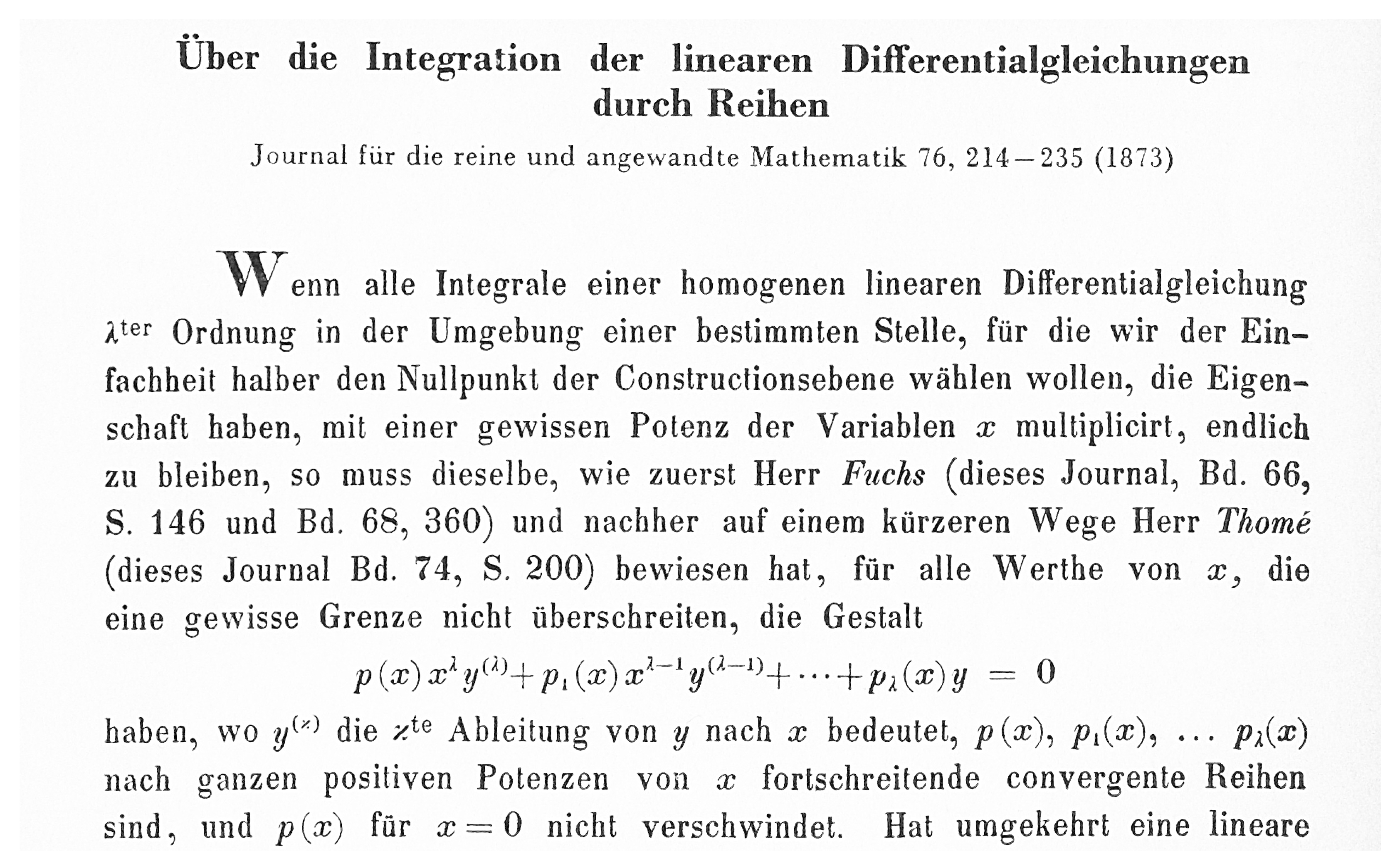
• The standardization of the differential equation by normalizing the pre-factor of $y^{″}$ to be $x^2$. In addition, see Figure 2.
• The Ansatz (5), inspired by the earlier results of Fuchs, to look for solutions in the form of generalized power series, while this generalization introduces no more than only a single parameter r. This parameter is used to shift the powers of the variable x in the power series, all by the same amount.
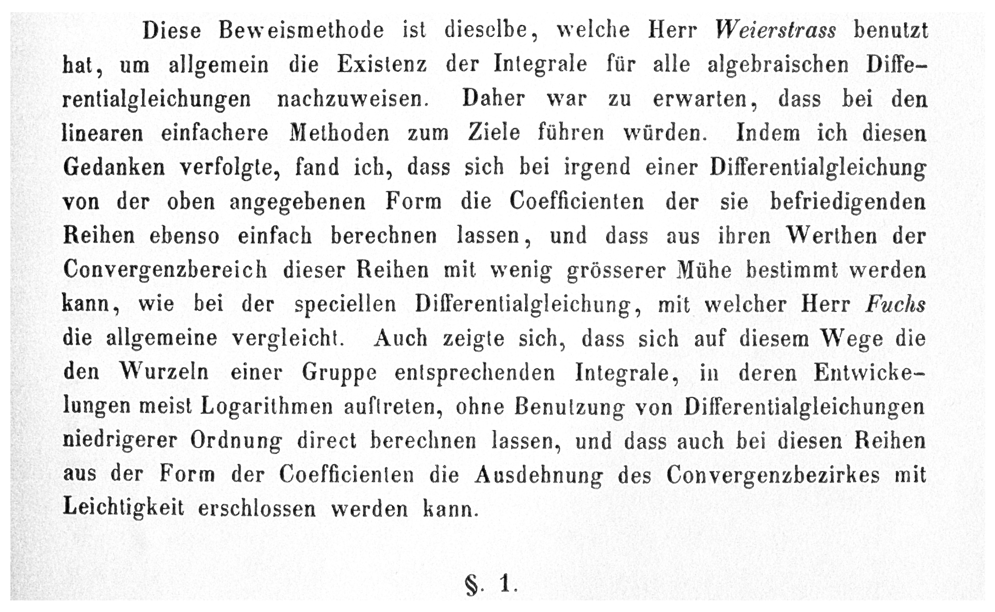
• Frobenius’ discovery that, at least for a first series solution, the coefficients $a_n$ of the series obey a recurrence relation that can be derived quite simply (“einfach”, see Figure 3).
• The idea that then all coefficients $a_n\left(r\right)$ of the series may be conceived as functions of r, too.
• As an attempt to construct solutions associated with a second root, $r_2$, of the indicial equation, in cases of roots $r_1$ and $r_2$ being equal or differing by an integer, Frobenius explored the consequences of choosing the leading coefficient $a_0\left(r\right)$ such that a division by zero in recurrence relations for the $a_n$ would be replaced by a limit process, ${lim}_{r\to r_2}$, so as to obtain finite values for all coefficients $a_n$. That is, in our phrasing, Frobenius explored the option to have

  $$a_0\left(r\right)=c_0(r-r_2),$$

  (56)

  instead of e.g., $a_0=1$.
• Frobenius’ idea that by means of differentiation with respect to r, new solutions of the differential equation can be obtained.

In his original manuscript [6], Frobenius actually took steps 1 to 5 all on the third and fourth page, immediately following his two-page introductory section. For what follows, it may be worth noting that step 6 was physically separated from the earlier steps by no less than five pages devoted to the proof of the convergence of solutions of type (5). Noting this may perhaps help to understand why, in the history of the method, step 6 was never before fully explored without first taking step 5, like we essentially did in our enhanced version of Frobenius’ method.

Step 5 was taken so as to obtain solutions of the differential equation, each of the form as proposed in step 2. Furthermore, the goal was to have one such a solution associated with each root of the indicial equation. The later discussion by Coddington [2] reflects the same purpose of step 5. Step 5 was documented indeed as being aiming at solutions in cases in which two roots $r_2$ and $r_1$ differ by an integer number, so when $r_1-r_2=N$.

Essentially to the end of obtaining a finite value for ${lim}_{r\to r_2}{a}_N\left(r\right)$, step 5 introduces a factor $r-r_2$ in $a_0\left(r\right)$. Although Frobenius’ limit procedure is effective in obtaining a solution associated with $r_2$ of the differential equation indeed, it actually only produces a solution that is linearly dependent on the first solution, $y(x,r_1)$, i.e., on the solution that had already been obtained, associated with $r_1$. This may well be perceived as a failed attempt to complete the set of fundamental solutions. However, for the overall understanding of the theory, the fact that in cases of $r_1-r_2=N$, the coefficient $a_N$ is in this sense associated with $y(x,r_1)$ is a key result. In our Section 2.3.2, we showed that one may naturally recover this result without Frobenius’ device, item 5 of our list, of choosing $a_0\left(r\right)\sim r-r_2$.

As we will document and discuss further in Section 4.3, the factor $r-r_2$ introduced through $a_0\left(r\right)$ in item 5, historically became a stowaway in the context of item 6, i.e., the technique of generating linearly independent solutions through differentiation with respect to r. As we shall discuss shortly, the introduction of the factor $r-r_2$ seems to have been in so far disadvantageous, that it seems to have delayed development of the tandem recurrence relations for the coefficients of solutions that we have developed and presented in the present manuscript.

In Section 3 we presented an illustration in support of this interpretation of the history of the subject, by deriving tandem recurrence relations for the coefficients of solutions of the second kind and integer and half-integer order of Bessel’s equation. Bessel functions of course are very well-known and vast amounts of results have been documented about them [4,16]. The tandem recurrence relations we presented here however, elementary as they seem to be, seem to not be widely known, if at all.

Lastly, we should mention consequences of the first item of our list, the normalization $\lambda \left(x\right)=1$ used by Frobenius and in textbooks on the subject ever since. As we highlighted in our exploration, whenever $\lambda \left(x\right)$, $p\left(x\right)$ and $q\left(x\right)$ are polynomials, as they often are in practical applications, we arrive at recurrence relations the number of terms of which are bounded, as a function of n. This boundedness is typically lost when $\lambda \left(x\right)$ is normalized.

4.3. The Role and History of the Factor $r-r_2$ in the Literature

As we saw in Section 4.2—see step 5 of our list of number steps in there—to search for solutions associated with $r_2$ and in case $r_1-r_2=N$, for non-zero integer N, Frobenius [6] took the initiative to set $a_0\left(r\right)$ proportional to a factor $r-r_2$. It is interesting that in our variant of the approach, we may recover this same proportionality of $a_0\left(r\right)$ to $r-r_2$, but only as a by-catch, after deriving the solutions of the differential equation. Indeed, along our approach, in first instance, according to relation (12) combined with ${\rho }^{\prime }\left(r_2\right)\ne 0$, to obtain a solution of the differential equation associated with $r=r_2$ no more is required than $a_0\left(r_2\right)=0$. To obtain more than a trivial solution from relation (28) then, we need $c_0\ne 0$. Combined with expression (27), finally this leads to the conclusion that $a_0\left(r\right)$ must depend on r, e.g., at its simplest, Equation (56):

$$a_0\left(r\right)=c_0(r-r_2).$$

Frobenius’ motivation for setting this from the onset was that, from expression (23) it is clear that, using (11) as a recurrence relation to obtain all the coefficients $a_n$, $0<n$, is problematic for $r=r_2$. Indeed, in case $n=N$, so to calculate $a_N$, the division by $\rho (n+r_2)$ needed to calculate the $a_n$, evokes division by $\rho (N+r_2)=\rho \left(r_1\right)$. That is, it would evoke a division by zero.

It was to remedy this division by zero that Frobenius [6] proposed to choose $a_0$ to be proportional to $r-r_2$. For then the recurrence relation (11) would imply all the $a_i$ to share this factor. The strategy was then to divide (11) by $\rho (n+r)$ to solve all the $a_n$, including $a_N$, as a function of r and then essentially to take the limit $r\to r_2$. Common factors $r-r_2$ in the $a_i$ and $\rho (N+r)$ would cancel, and a finite value for $a_N$ would be obtained. This procedure is also documented in detail by Coddington [2] and it seems to be the origin of the factors $r-r_2$ in the formulae proposed by Boyce and DiPrima in their presentation of these matters in their textbook on differential equations [3]. Indeed, instead of our relation (27), Boyce and DiPrima have

$$c_n\left(r_2\right)=\frac{d}{dr}\left[(r-r_2)a_n\left(r\right)\right]{|}_{r=r_2};\mathbf{NB}:\mathrm{with} a_0=1 \mathrm{and} a_n\left(r\right) \mathit{must} \mathit{be} \mathit{explicit}.$$

(57)

We have added the warning that $a_n\left(r\right)$ here must be an explicit function of r, so it may no longer recurrently depend on previous coefficients $a_i$, $i<n$. This will be explained shortly but it is usually prohibitive to application of relation (57). Indeed, it would be required to actually solve the recurrence relation for the $a_n\left(r\right)$, which is usually insurmountable [5].

Boyce and DiPrima did actually not include a derivation of their formula (57) in their textbook; for this, they referred to Coddington [2]. Coddington did actually not present Equation (57) at all, but his textbook does contain relation (13), with $r=r_2$. With (26), however, this suggests our (27), rather than (57).

The difference between our (27) and Boyce and DiPrima’s (57), i.e., the factor $r-r_2$, can be explained by interpreting $a_n\left(r\right)$ in (57), like the $a_n\left(r_1\right)$, to have been calculated from (11) with the standard choice $a_0\left(r\right)=1$; this latter value for $a_0$ is indeed documented, by Boyce and DiPrima. For any choice of $a_0\left(r_2\right)$, however, all $a_n\left(r_2\right)$ would be proportional to $a_0\left(r_2\right)$, and so the factor $r-r_2$ can be included after solving the $a_n\left(r_2\right)$ from (11) with $a_0\left(r_2\right)=1$. This apparently was done and therefore the factor $r-r_2$ appears in formula (57).

Boyce and DiPrima’s substitution of $(r-r_2)a_0$ for their original $a_0=1$, in the limit $r\to r_2$ effectively implements our $a_0\left(r_2\right)=0$ of (24). Thus, Boyce and DiPrima’s expression (57) is correct. They have documented how to successfully apply it indeed, to derive the coefficients for a second independent solution of Bessel’s equation of order one: this is one of the exercises in their section on this Bessel equation. Watson [4] recommended, but did not document, this approach to obtain these solutions of Bessel’s equation of order one; Watson identified the approach as being essentially Frobenius’ method and attributed application of it to Bessel’s equation to Forsyth [1]. The presentation by Boyce and DiPrima truthfully follows these originals. In this approach, the $a_n\left(r\right)$ are indeed first explicitly solved from (11). Application of (57) directly to such an intermediate result would indeed give correct coefficients $c_n$.

At this point, we need to emphasize however, that the factor $r-r_2$ in (57) does prohibit a recursive interpretation of the $c_n$ of (57): indeed, with a recursive interpretation, the $c_n$ would be multiplied by $r-r_2$ once again at each recursive step. This is clearly not intended and would obviously lead to erroneous results.

In contrast to this, our formulation, relations (28) and (11) can be applied fully recursively, without any need to obtain a non-recursive, explicit expression for the $a_n\left(r\right)$. This renders our approach generally applicable, i.e., a genuine method. Along this route we naturally find the tandem recurrence relations for the coefficients of the so-called exceptional, but practically important solutions of the differential equation, a result that, following the procedure as suggested by relation (57), hitherto seems to have been beyond reach.

5. Conclusions

The key result of the work presented here is the following. In Section 2 we enhanced Frobenius’ method by augmenting it with tandem recurrence relations that render all coefficients for those solutions of linear, second order differential equations about their regular singular points that may involve logarithmic terms. These tandem recurrence relations can be constructed by our enhanced variant of Frobenius’ method, exploring derivatives with respect to a parameter r. This parameter r corresponds to a shift of all the powers of the variable x in generalized power series, (5): Frobenius’ Ansatz.

Besides generalized power series, a logarithmic term may indeed appear in the solutions of a differential equation; the coefficient of this logarithmic term may vanish in certain cases. Hence this coefficient is of significant interest for applications in e.g., physics. Our enhanced variant of the theory naturally enables calculation of this coefficient of the logarithmic term, i.e., it provides a diagnostic tool to decide whether or not there does appear a logarithmic term.

Our avoiding of a normalization of the coefficient of the highest order derivative in the differential equation, $\lambda \left(x\right)$, led to a slight generalization of Frobenius’ original central formulae. As we showed however, in practical applications, the implied simplification of the recurrence relations can be very substantial.

The historical fact that these results seem not to have been established earlier seems surprising and calls for an explanation. As we discussed, it may well be that Frobenius’ initiative [6] to explicitly introduce a factor $r-r_2$, through $a_0\left(r\right)$, in his first attempt to derive a second independent solution of the form (5) through a limit procedure, may in the end have raised a stumbling block that has persisted in the subsequent literature for a long time. Frobenius’ idea that a way forward was to let the coefficients $a_n$ depend on r was priceless. In as far as we have derived any new result in the present manuscript, still it was derived from this powerful idea. Frobenius also proposed an adequate dependence of $a_0$ on r, in the exceptional cases $r_1-r_2=N$: we did in the end recover Frobenius’ factor $r-r_2$ in $a_0\left(r\right)$. However, this factor turns out not to play the role Frobenius seems to have had in mind. In Frobenius’ manuscript, the purpose of the factor $r-r_2$ was to cancel a division by zero, so as to obtain a finite value for $a_N$ or $c_N$. In our variant of Frobenius’ method, the role of the factor $r-r_2$ is to reconcile the facts that to support a second independent solution of the differential equation, associated with $r_2$, $a_0$ needs to vanish and $c_0$ should not vanish, while $c_0$ is the derivative of $a_0$ with respect to r.

References

1. Forsyth, A.R. A Treatise on Differential Equations; MacMillan and Co, Limited: New York, NY, USA, 1903. [Google Scholar]
2. Coddington, E.A. An Introduction to Ordinary Differential Equations; Prentice-Hall: Hoboken, NJ, USA, 1961. [Google Scholar]
3. Boyce, W.E.; DiPrima, R.C. Elementary Differential Equations and Boundary Value Problems, 11th ed.; Wiley: Hoboken, NJ, USA, 2013; Chapter 5.6. [Google Scholar]
4. Watson, G. A Treatise on the Theory of Bessel Functions; Cambridge University Press: Cambridge, UK, 1944. [Google Scholar]
5. Goode, S.; Annin, S. Differential Equations and Linear Algebra; Pearson: London, UK, 2014. [Google Scholar]
6. Frobenius, F.G. Über die Integration der linearen Differentialgleichungen durch Reihen. In Gesammelte Abhandlungen; Serre, J.P., Ed.; Springer: Berlin/Heidelberg, Germany, 1968; Volume 1, pp. 84–105. [Google Scholar]
7. Ince, E. Ordinary Differential Equations; Longmans, Green and Co., Ltd.: London, UK, 1927. [Google Scholar]
8. Coddington, E.A.; Levinson, N. Theory of Ordinary Differential Equations; Int. Series in Pure and Applied Mathematics; McGraw-Hill: New York, NY, USA, 1955. [Google Scholar]
9. Butkov, E. Mathematical Physics; Addison-Wesley: Boston, MA, USA, 1968. [Google Scholar]
10. Brannan, J.R.; Boyce, W.E. Differential Equations, with Boundary Value Problems, 2nd ed.; Wiley: Hoboken, NJ, USA, 2011; Chapter 8.6. [Google Scholar]
11. Fuchs, L.I. Zur Theorie der linearen Differentialgleichungen mit veränderlichen Coefficienten. In Gesammelte Mathematische Werke von L. Fuchs; Fuchs, R., Schlesinger, L., Eds.; University of Michigan Library: Berlin, Germany, 1865; Volume I, Chapter Jahrsber. Gewerbeschule; pp. 111–158. [Google Scholar]
12. Fuchs, L.I. Zur Theorie der linearen Differentialgleichungen mit veränderlichen Coefficienten. J. Reine Angew. Math. 1866, 66, 159–204. [Google Scholar]
13. van der Toorn, R. The Singularity of Legendre Functions of the First Kind as a Consequence of the Symmetry of Legendre’s Equation. Symmetry 2022, 14, 741. [Google Scholar] [CrossRef]
14. Thomé, L.W. Zur Theorie der Linearen Differentialgleichungen. J. Reine Angew. Math. 1872, 74, 193–217. [Google Scholar]
15. Gray, J. Linear Differential Equations and Group Theory from Riemann to Poincaré; Birkhäuser: Boston, MA, USA, 1986; ISBN 0-8176-3318-9. [Google Scholar]
16. Abramowitz, M.; Stegun, I.A. Handbook of Mathematical Functions; Dover: New York, NY, USA, 1964. [Google Scholar]
Figure 1. The title and opening sentence of Frobenius’ original paper on series solutions of linear differential equations [6]. Note that, as in the works of Fuchs [11,12], differential equations of n-th order were addressed, in full generality. To avoid prolixity and to allow focus instead, in our manuscript here, we restrict our coverage to second order equations. Frobenius introduced the name P ( y ) for the left hand side of the equation shown here. This corresponds to our linear operator L, i.e., to our expression (2).
Axioms 12 00032 g001
Figure 2. Frobenius’ Ansatz, our Equation (5), as published in 1873 [6], at the top of the third page of his paper. This fragment also contains the choice to normalize the coefficient of the highest order derivative, i.e., to set “ p ( x ) = 1 ”, Zur Vereinfachung der Beweise (“To simplify the proof”).
Axioms 12 00032 g002
Figure 3. Closing paragraph of the opening section of Frobenius’ seminal paper on series solutions [6]. While paying due respect to the earlier works of Weierstrass and Fuchs, Frobenius explained that he believed his own approach offered a worthwhile alternative, because of its simplicity (“ …einfach …”), ease (“ …mit Leichtigkeit …”) and directness (“ …direct …”). Three decades later, Forsyth ([1], Chap. VI) would indeed recommend Frobenius’ process, because of these merits.
Axioms 12 00032 g003
Disclaimer/Publisher’s Note: The statements, opinions and data contained in all publications are solely those of the individual author(s) and contributor(s) and not of MDPI and/or the editor(s). MDPI and/or the editor(s) disclaim responsibility for any injury to people or property resulting from any ideas, methods, instructions or products referred to in the content.