4.1. General Results
Out of the 25 groups initially formed, 23 finally reached an agreement and successfully submitted a survey.
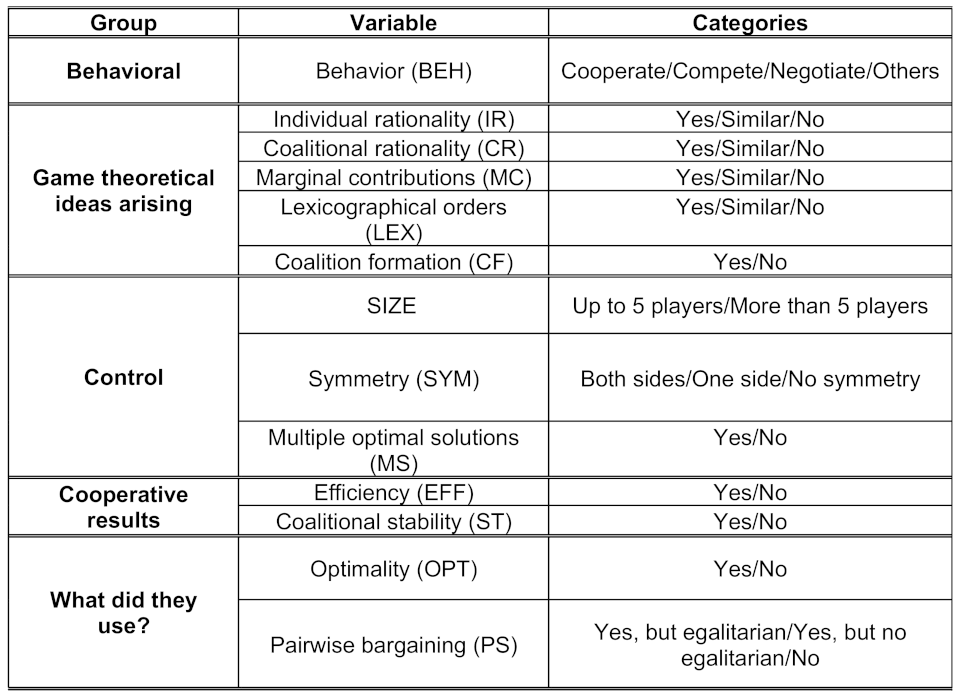
Table 2 summarizes the results. The most frequent process was a two-stage negotiation. It was followed by 10 groups. In a first stage, the pattern of trade was established, reaching in the majority of cases an optimal solution. In the second stage, negotiations took place within producer–retailer pairs to determine the split of the surplus generated from trade. The second and third most frequent patterns followed were the simultaneous determination of quantities traded and surplus sharing (four groups), or directly, a negotiation on the split of the surplus corresponding to the optimal solution (four groups). In fewer cases (three groups), coalitions were formed to decide collectively on the quantities and shares for a single player. Finally, two groups decided cooperatively on the quantity traded, although negotiation took place individually within producer–retailer pairs.
Relevant cooperative game-theoretic concepts, such as individual rationality, coalition rationality and marginal contributions, were totally absent from the reports submitted. Only in eight reports bargaining followed a lexicographic ordering of solutions, whereas in four cases, coalitions were explicitly mentioned. In 19 reports the outcome reached was an efficient solution. Moreover, in 11 groups, the split of profits satisfied the core of the underlying game.
Table 3 summarizes.
Regarding the emergence of cooperative results, in 19 groups ( of the cases) the final distribution of surplus was efficient. As we will argue below, the four cases where the distribution of surplus was inefficient relate to the nature of the transportation problem. Despite the fact that no reference was made in any of the reports to any concept analogous to coalition rationality, in 11 groups (), distributions were in the core of the corresponding cooperative game. It is also interesting to note the pervasive use of pairwise negotiations, observed in 20 groups ().
4.2. Analysis of Relations between Variables
In this subsection we explore the extent to which variables defined in the experiment are related with each other. To do so, we follow two measures. First, we present the Lambda Goodman and Kruskal analysis (Goodman and Kruskal [
18]), which reports the predictive capacity between variables. Second, we present the values of Cramèr’s V ([
19]), reporting the association (if any) between variables. Both techniques are presented in the symmetric and the asymmetric versions. The asymmetric version matches each explanatory variable (our control variables) and each response variable (the rest of the variables). In the symmetric version, cross-relations between response variables were measured.
Lambda values (see
Table 4 and
Table 5) account for the reduction in the prediction error when there is perfect knowledge of other variables involved in the study. It takes values on the unit interval, where
zero represents a null reduction and
one a full reduction. The values of Cramèr’s V (see
Table 6 and
Table 7) also lie between
zero (which means independence) and
one (which means full association). In brackets, the
p-values corresponding to the Chi-square tests. We also parametrized values inside the interval (according to the values obtained): values in
imply a low association; values between
an intermediate or moderate association; values in
imply a high association; finally values, in
imply a very high association.
Table 4 and
Table 6 contain the asymmetric analysis (i.e, the relation between control and other variables). First, it is interesting to note that when the transportation problem has multiple solutions, we can reduce the prediction error when pairwise bargaining takes place by 25% (see
Table 8). Therefore, multiple solutions and pairwise bargaining are somehow related. This is also confirmed when we look at
Table 6, where Cramèr’s V (
) reveals a statistically significant association between these two variables. Second, the relation between MS and LEX is also relevant. Although the Goodman and Kruskal’s asymmetric Lambda is zero (which means that ex ante knowledge of the MS category does not reduce the prediction error of the most likely result in variable LEX), Cramèr’s V (
) reveals a moderate statistically significant association between these two variables. The intuition behind this is that when there are multiple optimal solutions, agents try to sort them in order to reach an agreement.
Table 5 and
Table 7 include the descriptive analysis of the remaining variables. We can observe some ex ante predictable relations between variables EFF and OPT; EFF and ST; and OPT and ST. In particular, the intensity between CF and PS is somehow spurious, due to the fact that, when a coalition is formed, the split of profit is not negotiated by pairs, whereas when a coalition is not achieved we observe a negotiation by pairs. More interesting relations are observed between PS and LEX. This can be explained because players who used some lexicographic idea also were involved in a negotiation of profits within producer–retailer pairs. Finally, we point out the relation between OPT and PS. This fact arose because an optimal solution always yields a pairwise negotiation.
4.3. Students’ Behavior
We report here students’ behavior. In our context, behavior describes the types of strategies that a student (or a coalition of students) followed when they defined a trading plan in order to capture as much as profits they could. We focus on the most interesting markets to highlight two facts: (1) how students manage conflict situations; and (2) it was not an objective of students to achieve a stable result. From an economic perspective, the indication is that students were not rational (i.e., they were not strictly profit maximizing). They used rather weaker principles instead of rationality, such as equity, reasonableness and accessibility. Moreover, players did not provide a stable result in general (notice that students in two markets did not achieve any result of distribution of profit after several rounds of negotiations. Thus, we are not able to evaluate any idea related to coalition rationality in those markets).
![Axioms 11 00397 i001 Axioms 11 00397 i001]()
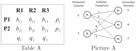
Students in Market 5 started by considering the four possible combinations of trading with an egalitarian distribution of profits:
| (x11, x12) | (7, 3) | (6, 4) | (5, 5) | (4, 6) |
| Distribution | (36.5;24.5,12) | (37;21,16) | (37.5;17.5,20) | (38;14,24) |
Secondly, they alternatively began to submit offers and counteroffers consisting on a trading plan and a profit distribution between producer–retailer pairs (this procedure was also used in three other markets). Only trading plans
and
were considered. After 23 bargaining rounds, they agreed to implement trading plan 4 with a distribution of profits
for
and
for
and
. However,
and
disagreed with the result; therefore,
offered to retailers half of their losses with respect to their best options. Finally, the distribution of profits was
and
for
; and for
was
and
; hence, there was a pie of
. This agreement corresponds to the equity principle in the following way:
| Player | ωi = Mi | ri = Mi − xi | ri/ωi |
| P1 | 47 | 9.75 | 0.21 |
| R1 | 24.5 | 5.25 | 0.21 |
| R2 | 24 | 4.5 | 0.19 |
where the standard of comparison is the best result obtained by each player throughout the negotiation process. Likewise, we observed that in the last step of the negotiation process, there were transference of profits (utility) from
to
and
. However, such a transfers were carried out through producer–retailer pairs.
Market 8 has only one optimal trading plan. Students took as a given this single plan, because it was the only way to obtain the maximum total profit. Hence, they negotiated between each producer–retailer pair under an optimal trading plan. This procedure was also used in another three markets. In this particular case, the final split of profit was the egalitarian distribution between each producer–retailer pair ().
Students in Market 15 agreed to cooperate and to distribute the total profit. As the total production was two units higher than the total demand, they implemented the trading plan symmetrically on both sides: , , and . However, lost out with it. Hence, they decided to divide the profit generated in each producer–retailer pair in an egalitarian way, except between pairs and ; in those cases, was endowed with , and was endowed with . Thus, the final distribution was (). This was done in order to compensate , and thus, students explicitly considered transference of utility (money). Something similar happened in another market with the same structure. However, in that case, students implemented the following trading plan in order to avoid complaints by the players: , and . The profit generated was 48. It was distributed in an egalitarian fashion. In order to maintain the structure of the problem, they divided the profit generated by each producer–retailer pair into . Once again, the players explicitly considered the possibility of transfer of utility (money) but respecting the matches given by the implemented trading plan.
In Market 16 students bargained for only one round. Then, retailers formed a coalition with a leader in order to negotiate with the producers. Finally, the retailers’ leader achieved a separate agreement with each producer, and the total profit obtained was split proportionally to their demands within the coalition. The final distribution of the total profit was (). Something similar happened in another two markets (in both cases with one producer and two retailers), but the total profit was first equally divided between the producer and the retailers, and thus split in the coalition proportionally to each demand.
Finally, the scheme in Market 18 had eight possible optimal trading plans. First, each student considered the eight optimal trading plans in terms of individual preferences according to their profit contributions in each optimal trading plan (the larger the contribution, the higher the opportunity of business). Thus, they obtained a system of preferences linked with the optimal solutions: the optimal solution minimizing the maximal loss (complaint). Therefore, they applied a lexicographic criterion to determine the implemented trading plan (something similar was also used in another 7 markets). Once the trading plan (in this case an optimal solution of the problem) was selected, they proceeded to negotiate the distribution of the profit by matching producer–retailer pairs in the selected trading. The following distribution of the total profit was obtained: (6.430, 4.445, 10.625; 9.000, 12.500). This procedure, selecting first the trading plan and then bargaining within each producer–retailer pair, was also used, in different ways, in another nine markets.


