A Stable Generalized Finite Element Method Coupled with Deep Neural Network for Interface Problems with Discontinuities

Abstract

The stable generalized finite element method (SGFEM) is an improved version of generalized or extended FEM (GFEM/XFEM), which (i) uses simple and unfitted meshes, (ii) reaches optimal convergence orders, and (iii) is stable and robust in the sense that conditioning is of the same order as that of FEM and does not get bad as interfaces approach boundaries of elements. This paper designs the SGFEM for the discontinuous interface problem (DIP) by coupling a deep neural network (DNN). The main idea is to construct a function using the DNN, which captures the discontinuous interface condition, and transform the DIP to an (approximately) equivalent continuous interface problem (CIP) based on the DNN function such that the SGFEM for CIPs can be applied. The SGFEM for the DIP is a conforming method that maintains the features (i)–(iii) of SGFEM and is free from penalty terms. The approximation error of the proposed SGFEM is analyzed mathematically, which is split into an error of SGFEM of the CIP and a learning error of the DNN. The learning dimension of DNN is one dimension less than that of the domain and can be implemented efficiently. It is known that the DNN enjoys advantages in nonlinear approximations and high-dimensional problems. Therefore, the proposed SGFEM coupled with the DNN has great potential in the high-dimensional interface problem with interfaces of complex geometries. Numerical experiments verify the efficiency and optimal convergence of the proposed method.

1. Introduction

Generalized or Extended Finite Element Methods (GFEM/XFEM) augment the standard FEM with special functions that mimic local features of exact solutions to solve complicated non-smooth engineering problems [1,2,3,4]. The applications of GFEM/XFEM to typical fields, such as crack problems, interface problems, and material failures are referred to [3,5,6,7,8,9,10,11,12,13]. Both GFEM and XFEM are based on a partition of unity [14,15,16] to “paste” the local special functions. We will use GFEM to represent the GFEM/XFEM below for simplicity. The GFEM has been extensively applied to the interface problem, including elliptic interface problems [11,17,18,19,20,21,22,23,24,25,26,27,28] and time-dependent interface problems [9,29,30,31,32,33,34]. Meshes used in the GFEM are simple, fixed, and independent of the location of interfaces so that remeshing or mesh refinement for the FEM are avoided in the GFEM.

It was realized quite early that the GFEM has a conditioning difficulty in that condition numbers of stiffness matrices may be much larger than those of the standard FEM, and the conditioning may get extremely bad as the interfaces approach the boundaries of elements. The bad conditioning is mainly caused by almost linear dependence between the FE functions and added special functions. Many interesting ideas have been proposed for the conditioning of GFEM, such as (a) locally adapting positions of either nodes or interface curves [32,35], preconditioning the stiffness matrices by employing domain decomposition [36], local Cholesky decomposition [5], condensing DOFs at certain nodes [37], and modifying the enriched functions based on orthogonalization [38]. Recently, a stable GFEM (SGFEM) was introduced in [1,6,39] to improve the conditioning of GFEM. The main idea of SGFEM is to modify enriched functions by subtracting its FE interpolant. The SGFEM has been applied to the crack problem [6,7,8] and interface problems [1,17,20,23,32,40]. The SGFEM for interface problems is proven to have the optimal convergence in [1,20], and the conditioning is of the same order as that of the FEM and does not deteriorate as the interfaces approach the boundaries of elements.

To the best of our knowledge, the SGFEM has been developed only for continuous interface problems. Interface problems can be categorized as continuous and discontinuous interface problems (CIPs/DIPs), characterized by ${\left[u\right]}_{\mathrm{\Gamma }}=0$ and ${\left[u\right]}_{\mathrm{\Gamma }}\ne 0$, respectively, where u is a solution to an interface problem with interface $\mathrm{\Gamma }$, and ${\left[u\right]}_{\mathrm{\Gamma }}$ is a jump of u across the interface $\mathrm{\Gamma }$. Both cases have many applications (see [11,22,23,32,34,41,42] for CIPs, [10,30,43,44,45,46] for DIPs). The shape functions in the SGFEM (also in some GFEM [3,9,11,17,20,23,25,31,32,34,41,42,47]) for the interface problem are continuous. Thus, the SGFEM can provide conforming approximations for CIPs. However, the continuous shape functions cannot be used directly for the DIP, and penalty techniques need to be employed typically [19,30,48]. We stress that many of the unfitted FEM or GFEM introduce penalty techniques and parameters to solve the CIP, such as [11,34,41,42]. It is possible to propose an SGFEM for DIPs by changing the enrichments and using the penalty technique above-mentioned. However, the penalty parameters are generally problem-dependent and difficult to choose in a uniform approach.

In this paper, we tend to design the SGFEM for DIPs free from penalty terms and parameters. The main idea is to transform a DIP into an equivalent CIP [45,46,49]. This can be achieved by deriving a function $\vartheta$ such that the modified solution $U=u-\vartheta$ satisfies the continuity condition ${\left[U\right]}_{\mathrm{\Gamma }}=0$. Unfortunately, such a $\vartheta$ is hard to construct, especially in the high dimensions where the interface has complex geometric shapes [45,49]. We construct such $\vartheta$ using the DNN. Then, the SGFEM for the CIP coupled with such $\vartheta$ is proposed for the DIP. This idea is motivated by recent pioneer research about solving partial differential equations (PDEs) using the DNN [50,51,52,53,54,55,56,57]. We mention that the DNN has also been applied to many engineering problems, for instance, energy approach [58], failure models and predictions [59,60,61]. We take a Poisson equation $-▵u=f$ in a domain $\Omega$, for example, which has an essential boundary condition $\overline{u}$ on $\partial \Omega$. The DNN for PDEs [53,54,55,57] is to minimize a loss function

$$\mathrm{Loss}=\frac{1}{2}{\int }_{\Omega }\nabla u·\nabla u-{\int }_{\Omega }fu+\beta {\int }_{\partial \Omega }{(u-\overline{u})}^2$$

(1)

using a certain DNN architecture, where $\beta$ is a parameter to balance the two terms in (1). The DNN method based on (1) is not convex, and does not show the convergence rate [53,55]. In addition, the essential boundary condition affects the accuracy DNN [53], and $\beta$ has to be selected carefully. To resolve the essential boundary condition, in [52,54,55], a small DNN is used to minimize the boundary term in (1), and then the PDE is transformed to an equivalent PDE with the (approximately) zero boundary condition, which is solved by another DNN. The small DNN function is defined in the whole domain $\Omega$, but only the values on $\partial \Omega$ are needed in the training process. Thus, such a DNN has a dimension number that is one dimension less than that of $\Omega$ and can approximate the boundary function efficiently, especially when the boundary $\partial \Omega$ has complex geometries [52,54,55]. This idea is adopted in this paper to address the discontinuous interface condition, i.e., ${\left[u\right]}_{\mathrm{\Gamma }}\ne 0$.

Specifically, we first use a small DNN to produce a function $\vartheta$ (defined in $\Omega$) by learning the discontinuous condition ${\left[u\right]}_{\mathrm{\Gamma }}$ such that ${\left[\vartheta \right]}_{\mathrm{\Gamma }}\approx {\left[u\right]}_{\mathrm{\Gamma }}$. As reported in [52,54,55], the jump ${\left[u\right]}_{\mathrm{\Gamma }}$ can be “learned” accurately and efficiently by the DNN. Then, the DIP is transformed to an (approximately) equivalent CIP based on $\vartheta$, which the SGFEM can solve for the CIP. The DNN function $\vartheta$ can be efficiently incorporated into the SGFEM framework because its differentiations are computed automatically. Since ${\left[\vartheta \right]}_{\mathrm{\Gamma }}$ does not equal ${\left[u\right]}_{\mathrm{\Gamma }}$ exactly, there is a conforming error in the SGFEM solution (combined with the DNN function $\vartheta$). This error is analyzed and proven mathematically, which indicates that the proposed SGFEM yields the optimal convergence for the DIP if the interface condition can be learned exactly enough. A set of numerical experiments verifies the theoretical results. It is known that the DNN possesses remarkable merits in solving high-dimensional problems and nonlinear approximations. Therefore, the proposed SGFEM in this paper has a great potential for the three-dimensional DIP with interfaces of complex geometries.

The paper is organized as follows. The model problem is described in Section 2. Conventional GFEM and SGFEM are reviewed in Section 3. The proposed SGFEM coupled with the DNN is proposed for the DIP in Section 4. In Section 5, we analyze the approximation error of the proposed method mathematically. The numerical experiments and concluding remarks are presented in Section 6 and Section 7, respectively.

2. Model Problem

For a domain $\Delta$ in ${\mathbb{R}}^2$, an integer m, and $1\le q\le \infty$, we denote the usual Sobolev spaces as $W^{m,q}(\Delta )$ with norm ${\parallel ·\parallel }_{W^{m,q}(\Delta )}$ and semi-norm ${|·|}_{W^{m,q}(\Delta )}$. The space $W^{m,q}(\Delta )$ will be represented by $H^m(\Delta )$ for $q=2$ and $L^q(\Delta )$ when $m=0$, respectively.

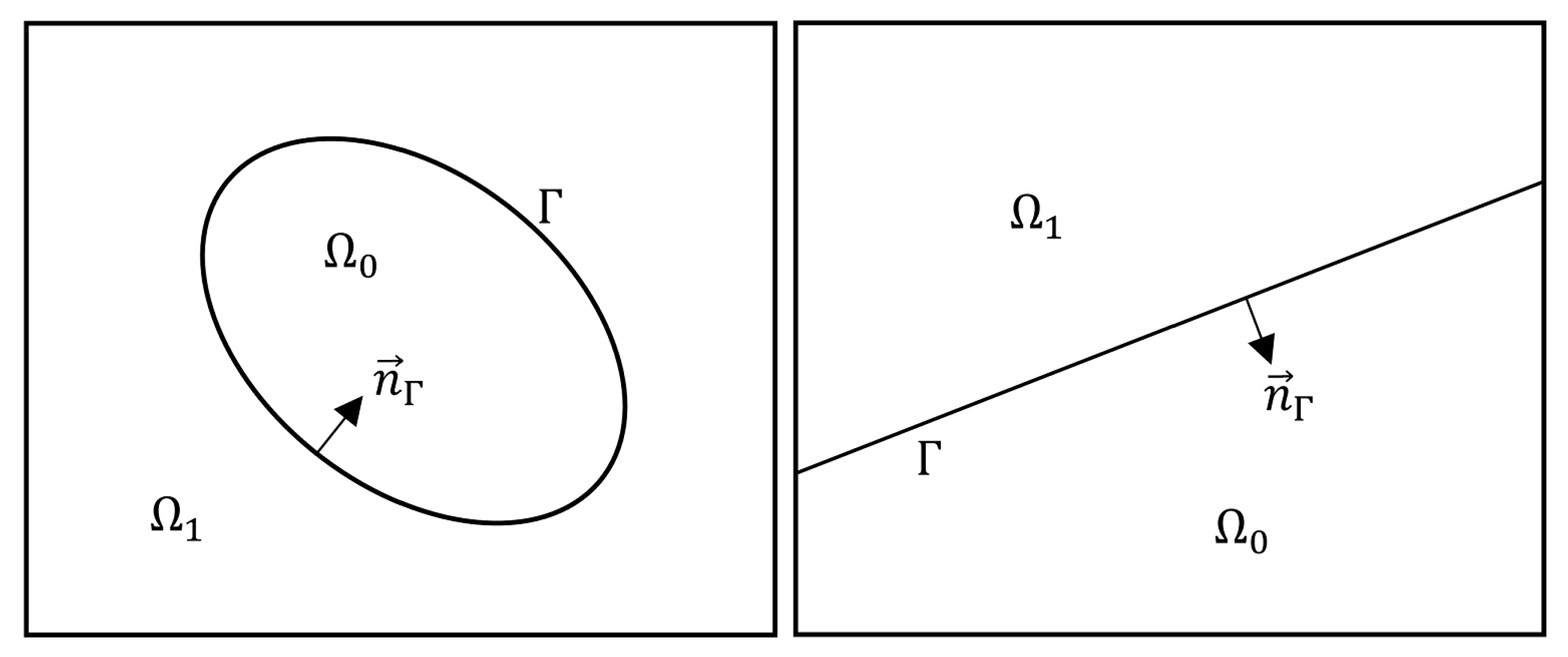
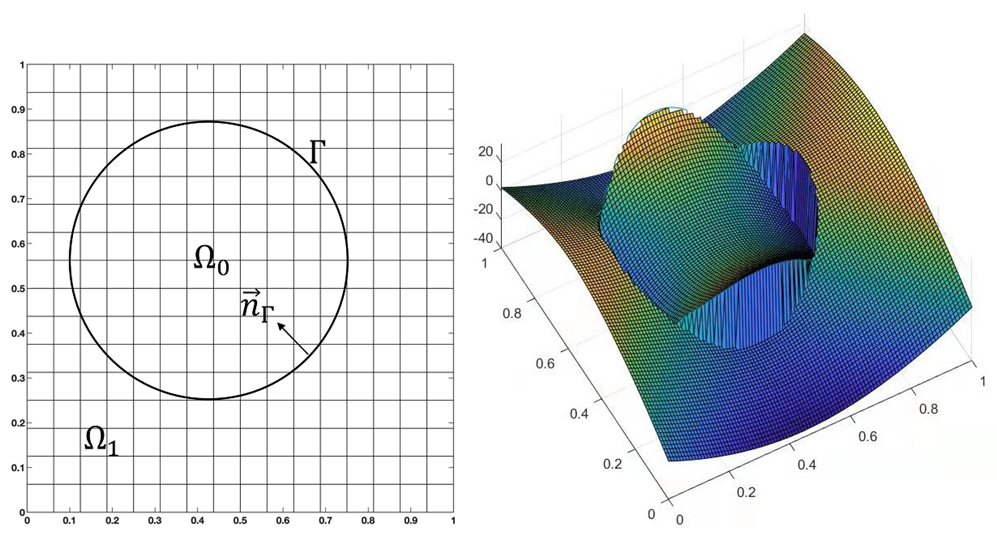
We consider a bounded and simply connected domain $\Omega \subset {\mathbb{R}}^2$ with a piecewise smooth boundary $\partial \Omega$. Let $\mathrm{\Gamma }$ be an interface that divides $\Omega$ into two domains ${\Omega }_0$ and ${\Omega }_1$ such that $\overline{\Omega }={\overline{\Omega }}_0\cup {\overline{\Omega }}_1$, ${\Omega }_0\cap {\Omega }_1=\varnothing$, and $\mathrm{\Gamma }={\overline{\Omega }}_0\cap {\overline{\Omega }}_1$. In this study, we consider smooth interfaces $\mathrm{\Gamma }$, as shown in Figure 1.

A point in the Cartesian coordinate system of ${\mathbb{R}}^2$ is denoted as $P=(x,y)$. Let a be a positive, piecewise-constant function given by

$$a\left(P\right)=\left\{\begin{array}{cc}{a}_0,\hfill & P\in {\Omega }_0,\\ a_1,\hfill & P\in {\Omega }_1,\end{array}\right.$$

(2)

where $a_0$ and $a_1$ are positive constants, $0<{\zeta }_0\le a_r\le {\zeta }_1<\infty ,r=0,1$, and ${\zeta }_0,{\zeta }_1\in \mathbb{R}$. Clearly, a is discontinuous along the interface $\mathrm{\Gamma }$.

We are interested in the solution u of the interface problem:

$$\begin{array}{ccc}\hfill -\nabla ·(a\nabla u)& =f,& \mathrm{in}\Omega ,\hfill \\ \hfill a\frac{\partial u}{\partial {\overrightarrow{n}}_b}& =g,& \mathrm{on}\partial \Omega ,\hfill \end{array}$$

(3)

subject to non-homogeneous jump conditions on the interface $\mathrm{\Gamma }$

$$\begin{array}{ccc}\hfill {\left[u\right]}_{\mathrm{\Gamma }}& =& \varphi ,\mathrm{on}\mathrm{\Gamma },\hfill \end{array}$$

(4)

$$\begin{array}{ccc}\hfill {\left[a\frac{\partial u}{\partial {\overrightarrow{n}}_{\mathrm{\Gamma }}}\right]}_{\mathrm{\Gamma }}& =& \psi ,\mathrm{on}\mathrm{\Gamma },\hfill \end{array}$$

(5)

where ${\overrightarrow{n}}_b$ and ${\overrightarrow{n}}_{\mathrm{\Gamma }}$ denote the unit outward normal to the boundary $\partial \Omega$ and the interface $\mathrm{\Gamma }$ directed towards ${\Omega }_0$, respectively. The notation ${\left[v\right]}_{\mathrm{\Gamma }}:=v_1-v_0$ defines the jump of a quantity v along the interface $\mathrm{\Gamma }$, where $v_r{:=v|}_{{\overline{\Omega }}_r},r=0,1$. We mention that if the boundary $\partial \Omega$ contains a re-entrant corner, u may be singular and may not belong to $H^2\left({\Omega }_r\right),r=0,1$. However, we do not discuss such a situation in this paper and limit the setting to the case $u\in H^2\left({\Omega }_r\right),r=0,1$, as in [42,45,47]. Therefore, we assume that the boundary $\partial \Omega$ and the data $f,g,\varphi$, $\psi$ are given such that the solution $u\in {\mathbb{M}}_2$, where ${\mathbb{M}}_2$ is defined by

$${\mathbb{M}}_2:={\{u:u|}_{{\Omega }_r}\in H^2\left({\Omega }_r\right),r=0,1\mathrm{and}\parallel {\partial }^{\alpha }{u\parallel }_{L^{\infty }\left(\mathrm{\Gamma }\right)}<\infty ,\left|\alpha \right|\le 1\}$$

(6)

with a norm

$${\parallel u\parallel }_{{\mathbb{M}}_2}=\parallel u_0{\parallel }_{H^2\left({\Omega }_0\right)}+\parallel u_1{\parallel }_{H^2\left({\Omega }_1\right)}+\sum _{\left|\alpha \right|\le 1}{\parallel {\partial }^{\alpha }u\parallel }_{L^{\infty }\left(\mathrm{\Gamma }\right)},\forall u\in {\mathbb{M}}_2.$$

The interface condition (4) has an essential effect on the features of the solution and constructions of numerical algorithms. The problem (3)–(5) is referred to as a CIP and a DIP if $\varphi$ in (4) is zero and nonzero, respectively. Both the CIP and DIP have many applications, see [11,22,23,32,34,41,42] for the CIP and [10,30,43,44,45,46] for the DIP. The SGFEM was proposed for the CIP to provide conforming approximations [17,20,23,27,40]. In this paper, the SGFEM is generalized to the DIP in a conforming approach that is free from any penalty terms.

3. Conventional Gfem and Sgfem for Interface Problems

We begin with a quasi-uniform finite element mesh ${\mathcal{T}}_h=\left\{e_s\right\}$ of the domain $\Omega$ with mesh size $0<h<1$, where the finite elements $e_s$ can be triangles or quadrilaterals. We note that the mesh ${\mathcal{T}}_h$ does not need to match the interface $\mathrm{\Gamma }$. Let ${\left\{P_i\right\}}_{i\in I_h}$ be the set of finite element nodes associated with the mesh ${\mathcal{T}}_h$, where $I_h$ is the index set of the nodes. For every $i\in I_h$, we consider the standard linear (bilinear for quadrilateral element) finite element hat function ${\varphi }_i$. The closure of support of ${\varphi }_i$ is denoted by ${\omega }_i$, which is called the patch associated with the node $P_i$. Since the mesh is quasi-uniform, we assume that

$$\parallel {\varphi }_i{\parallel }_{L^{\infty }(\Omega )}=\parallel {\varphi }_i{\parallel }_{L^{\infty }\left({\omega }_i\right)}\le 1,\parallel \nabla {\varphi }_i{\parallel }_{L^{\infty }(\Omega )}={\parallel \nabla {\varphi }_i\parallel }_{L^{\infty }\left({\omega }_i\right)}\le C{h}^{-1},$$

(7)

where the positive constant C is independent of h and i. It is well known that ${\left\{{\varphi }_i\right\}}_{i\in I_h}$ form a partition of unity (PU) [14,15,16] subordinate to the patches ${\left\{{\omega }_i\right\}}_{i\in I_h}$.

The standard FEM subspace to approximate the solution of (3) is given by

$$S_h:=S_{FEM}=\mathrm{span}\{{\varphi }_i\left(x\right):i\in I_h\}.$$

(8)

The FEM yields highly accurate approximations only if the underlying variational problem has a smooth solution. However, it is also well known that an FEM with a quasi-uniform mesh cannot approximate the solution of the interface problem efficiently [23,47].

The generalized or extended FEM (GFEM) [2,3] is a typical technique to approximate the non-smooth solutions to variational problems. The approximation space $S_h$ of GFEM is obtained by augmenting the finite element space $S_{FEM}$ by non-polynomial enrichment space $S_{ENR}$ using the enrichment functions ${\Pi }_i$ as follows:

$$S_h=S_{FEM}\oplus S_{ENR}\mathrm{and}{S}_{ENR}=\mathrm{span}\{{\varphi }_i{\Pi }_i:i\in I_{h,enr}\mathrm{and}{I}_{h,enr}\subset I_h\},$$

(9)

where the enrichment functions ${\Pi }_i$ are problem-dependent and mimic the non-smooth exact solutions of the underlying variational problem. The nodes indexed by $I_{h,enr}$, are called the enriched nodes. The choice of $I_{h,enr}\subset I_h$ can vary and may also be problem-dependent.

The enrichment functions ${\Pi }_i$ used in the GFEM to approximate the solution of a smooth interface problem are generally based on a distance function (or absolute of level set function) [3,18,23]

$$D\left(P\right)=\mathrm{dist}(P,\mathrm{\Gamma }).$$

In a conventional GFEM for the interface problems, the approximate subspace is

$$S_h=S_{FEM}\oplus S_{ENR}\mathrm{and}{S}_{ENR}=\mathrm{span}\{{\varphi }_{i}D:i\in I_{h,enr}=I_{h,enr}^{\mathrm{\Gamma }}\},$$

(10)

and

$$I_{h,enr}^{\mathrm{\Gamma }}=\{i\in I_h:P_i\in e_s\mathrm{where}{\mathring{e}}_s\cap \mathrm{\Gamma }\ne \varnothing \}.$$

It is easy to know that

$$\mathrm{Card}\left(I_{h,enr}^{\mathrm{\Gamma }}\right):=\mathrm{cardinality} \mathrm{of} I_{h,enr}^{\mathrm{\Gamma }}=O\left(h^{-1}\right).$$

(11)

The GFEM based on $I_{h,enr}^{\mathrm{\Gamma }}$ is referred to as a topological GFEM [3]. It was known early (e.g., [23]) that the topological GFEM only produces the convergence order $O\left(\sqrt{h}\right)$ in energy norm, which is not optimal $O\left(h\right)$. The optimal convergence can be attained by the geometric GFEM [3,23] and corrected GFEM [3,22]. However, the geometric GFEM introduces many more enriched degrees of freedom (DOFs) than the topological ones, and its conditioning is of $O\left(h^{-4}\right)$ [23] that is much higher than that of the FEM. Meanwhile, the conditioning of the corrected GFEM may not be stable because it may “blow up” as the interface $\mathrm{\Gamma }$ is close to the nodes of the mesh [27].

Recently, a simple local procedure of subtracting the interpolant was introduced in [1,6,17,20,23,39,40] to address the bad conditioning of GFEM, and the modified GFEM is referred to as a stable GFEM (SGFEM). Specifically, the approximate subspace of the SGFEM for the interface problems is given by

$$S_h=S_{FEM}\oplus S_{ENR}\mathrm{and}{S}_{ENR}=\mathrm{span}\{{\varphi }_i(D-{\mathcal{I}}_{h}D):i\in I_{h,enr}=I_{h,enr}^{\mathrm{\Gamma }}\},$$

(12)

where ${\mathcal{I}}_{h}f$ is the FEM interpolant of a continuous function f based on $S_{FEM}$. It was shown [17] that the SGFEM (12) for the elliptic interface (a) reaches the optimal convergence order $O\left(h\right)$ in energy norm, (b) has a scaled condition number (SCN) of stiffness matrices $O\left(h^{-2}\right)$ that is of the same order as the FEM, and (c) is robust in that the convergence and SCN do not depend on the relative positions of the mesh and interfaces.

Remark 1.

We mention that there are other options for the enrichments of the GFEM of the interface problems, such as [11,41,48], where

$${\mathrm{\Pi }}_i=H$$

is used as the enrichments, and H is the Heaviside function 1 in ${\Omega }_0$ and $-1$ in ${\Omega }_1$. This scheme leads to a non-conforming formulation because of the discontinuity of H. A penalty technique needs to be developed to deal with discontinuity. This paper presents conforming methods in which the variational formulations are standard without any penalty terms or parameters.

We next illustrate the scaled condition number (SCN) of the stiffness matrices of the GFEM or SGFEM. For simplicity, we re-arrange the order of the shape functions so that the stiffness or mass matrices $\mathbf{B}$ of GFEM have the form

$$\mathbf{B}=\left[\begin{array}{cc}{\mathbf{B}}_{11}& {\mathbf{B}}_{12}\\ {\mathbf{B}}_{12}^T& {\mathbf{B}}_{22}\end{array}\right],$$

(13)

where ${\mathbf{B}}_{11}$ and ${\mathbf{B}}_{22}$ are associated with the FE part and the enrichment part of GFEM or SGFEM, respectively. We note that ${\mathbf{B}}_{11}$ is the standard finite element matrix with respect to the standard finite element triangulation used to define the GFEM. Consider the matrix

$$\mathbf{D}=\left[\begin{array}{cc}{\mathbf{D}}_{11}& 0\\ 0& {\mathbf{D}}_{22}\end{array}\right],$$

where ${\mathbf{D}}_{11}$ and ${\mathbf{D}}_{22}$ are diagonal matrices with

$${\left({\mathbf{D}}_{11}\right)}_{ii}={\left({\mathbf{B}}_{11}\right)}_{ii}^{-1/2}\mathrm{and}{\left({\mathbf{D}}_{22}\right)}_{ii}={\left({\mathbf{B}}_{22}\right)}_{ii}^{-1/2}.$$

(14)

We define $\widehat{\mathbf{B}}:=\mathbf{D}\mathbf{B}\mathbf{D}$ and ${\widehat{\mathbf{B}}}_{11}:={\mathbf{D}}_{11}{\mathbf{B}}_{11}{\mathbf{D}}_{11}$. The SCNs of $\mathbf{B}$ and ${\mathbf{B}}_{11}$ are defined by

$$\mathcal{K}:=\kappa \left(\widehat{\mathbf{B}}\right),{\mathcal{K}}_{FEM}:=\kappa \left({\widehat{\mathbf{B}}}_{11}\right),$$

respectively, where $\kappa \left(\mathbf{B}\right)$ is a condition number of a matrix $\mathbf{B}$. It is known that ${\mathcal{K}}_{FEM}=O\left(h^{-2}\right)$ for the stiffness matrices of FEM.

The relevant difficulties of GFEM consist of (i) stability: $\mathcal{K}$ may be much bigger than ${\mathcal{K}}_{FEM}$, and (ii) robustness: $\mathcal{K}$ may blow up as the interfaces are close to the boundaries of elements [1,2,3,23]. These are caused by the almost linear dependence of subspaces $S_{FEM}$ and $S_{ENR}$. The SGFEM is the stable and robust GFEM, and has been applied to crack and interface problems successfully [1,6,17,20,23,39,40].

The convergence of SGFEM for the CIP

The SGFEM for the CIP has been studied in [17,23,27,40], and the associated variational formulation based on the SGFEM space (12) is as follows:

$$\mathrm{Find}{u}_{SG,h}\in S_h\mathrm{such} \mathrm{that}B(u_{SG,h},v_h)=L\left(v_h\right),\forall v_h\in S_h,$$

(15)

where

$$B(u,v):={\int }_{\Omega }a\nabla u·\nabla vdP,L\left(v\right)={\int }_{\Omega }fvdx+{\int }_{\partial \Omega }gvds+{\int }_{\mathrm{\Gamma }}\psi vds.$$

(16)

We define $\mathcal{E}(\Omega )$ to be the energy space with respect to the CIP given by

$$\mathcal{E}(\Omega ):=\{u\in H^1(\Omega ):\parallel u{\parallel }_{\mathcal{E}(\Omega )}^2:=B(u,u)<\infty \mathrm{and}{\left[u\right]}_{\mathrm{\Gamma }}=0on\mathrm{\Gamma }\}.$$

(17)

It is obvious that ${\mathbb{S}}_h$ (12) belongs to $\mathcal{E}(\Omega )$. The convergence of $u_{SG,h}$ to u was proven in [17,27,40], and we present it here without its proof.

Theorem 1.

Suppose that $u\in {\mathbb{M}}_2$ is the solution of the CIP ((3)–(5) with $\varphi =0$), and $u_{SG,h}$ is the SGFEM solution of (15) based on the finite-dimensional subspace $S_h$ (12), then there exists $C>0$ independent of h such that

$$\parallel u-u_{SG,h}{\parallel }_{\mathcal{E}(\Omega )}\le Ch{\parallel u\parallel }_{{\mathbb{M}}_2}.$$

(18)

In the next section, the SGFEM of the CIP is generalized to the DIP in a conforming approach that is free from any penalty terms by coupling a DNN.

4. Sgfem Coupled with Dnn for Dip

We first employ the DNN to learn a function that approximates the discontinuous interface condition. Then, by coupling with the DNN function, we reformulate the DIP into an (approximately) equivalent continuous model, which can be solved by SGFEM.

Let ${\vartheta }_0$ be a function in $H^2\left({\Omega }_0\right)$ with

$${\vartheta }_0{|}_{\mathrm{\Gamma }}=-\varphi .$$

(19)

Define $\tilde{u}$ to be a function on $\Omega$ as

$$\tilde{u}=\left\{\begin{array}{cc}{\vartheta }_0,\hfill & \mathrm{in}{\overline{\Omega }}_0,\hfill \\ 0,\hfill & \mathrm{in}{\Omega }_1,\hfill \end{array}\right.$$

(20)

then $\tilde{u}$ satisfies the interface problem (4) because ${\left[\tilde{u}\right]}_{\mathrm{\Gamma }}=0-{\vartheta }_0{|}_{\mathrm{\Gamma }}=0-(-\varphi )=\varphi$. Define a function $\tilde{U}=u-\tilde{u}$, then

$$\tilde{U}=\left\{\begin{array}{cc}{u}_0-{\vartheta }_0,\hfill & \mathrm{on}{\Omega }_0,\hfill \\ u_1,\hfill & \mathrm{on}{\Omega }_1.\hfill \end{array}\right.$$

(21)

It is easy to check that the $\tilde{U}$ satisfies the continuous interface problem, i.e., ${\left[\tilde{U}\right]}_{\mathrm{\Gamma }}={\left[u\right]}_{\mathrm{\Gamma }}-{\left[\tilde{u}\right]}_{\mathrm{\Gamma }}=0$. The model problem (3) with the discontinuous interface conditions (4) and (5) is transformed into an equivalent equation about $\tilde{U}$ with the continuous interface condition:

$$\begin{array}{ccc}\hfill -\nabla ·(a\nabla \tilde{U})& =& f+\nabla ·(a\nabla \tilde{u}),in\Omega ,\hfill \end{array}$$

(22)

$$\begin{array}{ccc}\hfill a\frac{\partial \tilde{U}}{\partial {\overrightarrow{n}}_b}& =& g-a\frac{\partial \tilde{u}}{\partial {\overrightarrow{n}}_b},on\partial \Omega ,\hfill \end{array}$$

(23)

$$\begin{array}{ccc}\hfill {\left[\tilde{U}\right]}_{\mathrm{\Gamma }}& =& 0,on\mathrm{\Gamma },\hfill \end{array}$$

(24)

$$\begin{array}{ccc}\hfill {\left[a\frac{\partial \tilde{U}}{\partial {\overrightarrow{n}}_{\mathrm{\Gamma }}}\right]}_{\mathrm{\Gamma }}& =& \psi -{\left[a\frac{\partial \tilde{u}}{\partial {\overrightarrow{n}}_{\mathrm{\Gamma }}}\right]}_{\mathrm{\Gamma }}=\psi +a_0\frac{\partial \tilde{u}}{\partial {\overrightarrow{n}}_{\mathrm{\Gamma }}},on\mathrm{\Gamma }.\hfill \end{array}$$

(25)

We note that the RHSs of (23)–(25) can be simplified because $\tilde{u}=0$ in ${\Omega }_1$, for instance, in the boundary condition (24) $g-a\frac{\partial \tilde{u}}{\partial {\overrightarrow{n}}_b}=g$ if $\mathrm{\Gamma }\subset \Omega$. The variational formula of (23)–(25) is the following:

$$\mathrm{Find}\tilde{U}\in \mathcal{E}(\Omega )\mathrm{such} \mathrm{that}B(\tilde{U},V)=\tilde{L}\left(V\right),\forall V\in \mathcal{E}(\Omega ),$$

(26)

where

$$\begin{array}{cc}\hfill \tilde{L}\left(V\right)& ={\int }_{\Omega }fVdP+{\int }_{{\Omega }_0}(a_0\Delta \tilde{u})VdP+{\int }_{\partial \Omega }gVds-{\int }_{\partial \Omega \cap \partial {\Omega }_0}{a}_0\frac{\partial \tilde{u}}{\partial {\overrightarrow{n}}_b}Vds+{\int }_{\mathrm{\Gamma }}\left(\psi -{\left[a_0\frac{\partial \tilde{u}}{\partial {\overrightarrow{n}}_{\mathrm{\Gamma }}}\right]}_{\mathrm{\Gamma }}\right)Vds\hfill \\ \hfill & ={\int }_{\Omega }fVdP+{\int }_{\partial \Omega }gV\mathrm{d}s+{\int }_{\mathrm{\Gamma }}\psi Vds+\left[{\int }_{{\Omega }_0}(a_0\Delta \tilde{u})VdP-{\int }_{\partial \Omega \cap \partial {\Omega }_0}{a}_0\frac{\partial \tilde{u}}{\partial {\overrightarrow{n}}_b}Vds+{\int }_{\mathrm{\Gamma }}{a}_0\frac{\partial \tilde{u}}{\partial {\overrightarrow{n}}_{\mathrm{\Gamma }}}Vds\right]\hfill \\ \hfill & ={\int }_{\Omega }fVdP+{\int }_{\partial \Omega }gV\mathrm{d}s+{\int }_{\mathrm{\Gamma }}\psi Vds-{\int }_{{\Omega }_0}{a}_0\nabla \tilde{u}·\nabla VdP,\hfill \end{array}$$

(27)

and $B(·,·)$ and $\mathcal{E}(\Omega )$ are defined in (16) and (17), respectively. Note that in the second equality of (27) ${\overrightarrow{n}}_{\mathrm{\Gamma }}$ is directed towards to ${\Omega }_0$.

We note that $\tilde{L}$ in variational formula (26) depends on the unknown $\tilde{u}$, and cannot be calculated. It is easy to see that the evaluations of $\tilde{u}$ on $\mathrm{\Gamma }$ (19) rather than in $\Omega$ are essential for the derivation of the equivalent CIP (23)–(25). This leads us to construct a function ${\tilde{u}}^{{\theta }_{\ast }}$ (defined in $\Omega$) using a DNN such that ${\tilde{u}}^{{\theta }_{\ast }}$ mimics the condition (19) with high precision, where ${\theta }_{\ast }$ are parameters in the DNN algorithm. Such a ${\tilde{u}}^{{\theta }_{\ast }}$ is available, and the associated variational formula is solvable.

To this end, we take $N_{\mathrm{\Gamma }}$ sampling points $Q_i$ uniformly distributed on $\mathrm{\Gamma }$. Let $X={\left[Q_i\right]}_{i=1}^{N_{\mathrm{\Gamma }}}$ and $Y={\left[\varphi \left(Q_i\right)\right]}_{i=1}^{N_{\mathrm{\Gamma }}}$ be the input and output sets, respectively, for training the DNN. The loss function for training the DNN is defined

$$\mathrm{Loss}(X;\theta )={\displaystyle \frac{1}{N_{\mathrm{\Gamma }}}}\sum _{i=1}^{N_{\mathrm{\Gamma }}}{\left[{\vartheta }^{\theta }\left(Q_i\right)-\left(-\varphi \left(Q_i\right)\right)\right]}^2,\forall {\vartheta }^{\theta }\in {\mathbb{S}}_{DNN},$$

(28)

where ${\mathbb{S}}_{DNN}$ is a subspace (defined in $\Omega$) generated by a DNN with parameters $\theta =\{W_i,b_i\}$; $W_i,b_i$ are the weights and bias in the DNN, respectively. A DNN function ${\vartheta }^{{\theta }_{\ast }}$ with certain parameter ${\theta }_{\ast }$ is obtained by solving the following minimization problem-based loss function (28):

$$\underset{{\vartheta }^{\theta }\in {\mathbb{S}}_{DNN}}{min}\mathrm{Loss}(X;\theta ).$$

(29)

${\vartheta }^{{\theta }_{\ast }}$ belongs to $C^2\left(\overline{\Omega }\right)$ if the aviation function is chosen as the Sigmoid function [62,63].

Similar with the definition of $\tilde{u}$ (20) we define a function on $\Omega$ as

$${\tilde{u}}^{{\theta }_{\ast }}=\left\{\begin{array}{cc}{\vartheta }^{{\theta }_{\ast }},\hfill & \mathrm{in}{\Omega }_0,\hfill \\ 0,\hfill & \mathrm{in}{\Omega }_1,\hfill \end{array}\right.$$

(30)

and the variational formula based on ${\tilde{u}}^{{\theta }_{\ast }}$ is proposed as follows:

$$\mathrm{Find}{\tilde{U}}^{{\theta }_{\ast }}\in \mathcal{E}(\Omega )\mathrm{such} \mathrm{that}B({\tilde{U}}^{{\theta }_{\ast }},V)={\tilde{L}}^{{\theta }_{\ast }}\left(V\right),\forall V\in \mathcal{E}(\Omega ),$$

(31)

where

$$\begin{array}{cc}\hfill {\tilde{L}}^{{\theta }_{\ast }}\left(V\right)& ={\int }_{\Omega }fVdP+{\int }_{{\Omega }_0}(a_0\Delta {\tilde{u}}^{{\theta }_{\ast }})VdP+{\int }_{\partial \Omega }gVds-{\int }_{\partial \Omega \cap \partial {\Omega }_0}{a}_0\frac{\partial {\tilde{u}}^{{\theta }_{\ast }}}{\partial {\overrightarrow{n}}_b}Vds+{\int }_{\mathrm{\Gamma }}\left(\psi -{\left[a_0\frac{\partial {\tilde{u}}^{{\theta }_{\ast }}}{\partial {\overrightarrow{n}}_{\mathrm{\Gamma }}}\right]}_{\mathrm{\Gamma }}\right)Vds\hfill \\ \hfill & ={\int }_{\Omega }fVdP+{\int }_{\partial \Omega }gV\mathrm{d}s+{\int }_{\mathrm{\Gamma }}\psi Vds-{\int }_{{\Omega }_0}{a}_0\nabla {\tilde{u}}^{{\theta }_{\ast }}·\nabla VdP,\hfill \end{array}$$

(32)

and the function $u^{{\theta }_{\ast }}:=U^{{\theta }_{\ast }}+{\tilde{u}}^{{\theta }_{\ast }}$ serves as the approximation solution to u. We stress that (31) is not equivalent to the initial problem (3) exactly because according to (28) and (29),

$${\left[{\tilde{u}}^{{\theta }_{\ast }}\right]}_{\mathrm{\Gamma }}=-{\vartheta }^{{\theta }_{\ast }}\approx (\ne )\varphi ,\mathrm{on}\mathrm{\Gamma }.$$

This conforming error will be analyzed in the next section.

Unlike the variational problem (26), the problem (31) is computable because ${\tilde{u}}^{{\theta }_{\ast }}$ is obtained using the DNN. The problem (31) is discretized using the SGFEM subspace for the CIP, and the associated variational problem is

$$\mathrm{Find}{\tilde{U}}_h^{{\theta }_{\ast }}\in {\mathbb{S}}_h\mathrm{such} \mathrm{that}B({\tilde{U}}_h^{{\theta }_{\ast }},V_h)={\tilde{L}}^{{\theta }_{\ast }}\left(V_h\right),\forall V\in {\mathbb{S}}_h.$$

(33)

Finally, $u_h^{{\theta }_{\ast }}:={\tilde{U}}_h^{{\theta }_{\ast }}+{\tilde{u}}^{{\theta }_{\ast }}$ serves as the approximation solution to the initial problem (3), and the approximation error of $u_h^{{\theta }_{\ast }}$ will be analyzed mathematically in the next section. The formula (33) is called the SGFEM coupled with the DNN for the DIP due to the introduction of the DNN function ${\tilde{u}}^{{\theta }_{\ast }}$.

Remark 2.

The idea to transform the DIP into a CIP using the DNN is motivated by [52,54,55]. In [52,54,55], non-homogeneous boundary conditions are transformed into homogeneous ones using a shallow DNN, and the associated (approximately) homogeneous equations are solved by another DNN. This approach has advantages over conventional methods (e.g., FEM, GFEM) in that it is meshless and can solve problems with boundaries of complex geometries, and is powerful for high-dimensional problems. We couple the SGFEM for the CIP with the shallow DNN to address the DIP in this paper. We achieve that (a) all the advantages of SGFEM are maintained for the DIP, (b) the proposed SGFEM for the DIP is a conforming method free from any penalty terms, and (c) the method has great potential for geometrically complex interfaces, especially in three dimensions (reported in a forthcoming study).

We analyze the computational costs of the proposed method (33). First, the stiffness matrices of (33) are exactly the same as those of SGFEM for the CIP, and only the RHS (32) of (33) needs to be treated. Therefore, the assembling of stiffness matrices and the construction of RHS can be implemented separately or in parallel. Second, the computational dimension of learning ${\vartheta }^{{\theta }_{\ast }}$ based on (29) is one dimension less than the space dimension because the sampling points are located in the interface curve, and the learning time is very little in comparison with the assembling of stiffness matrices. Moreover, automatic differentiations are available in the existing DNN frameworks to save computational time. Therefore the proposed SGFEM coupled with the DNN is computationally efficient.

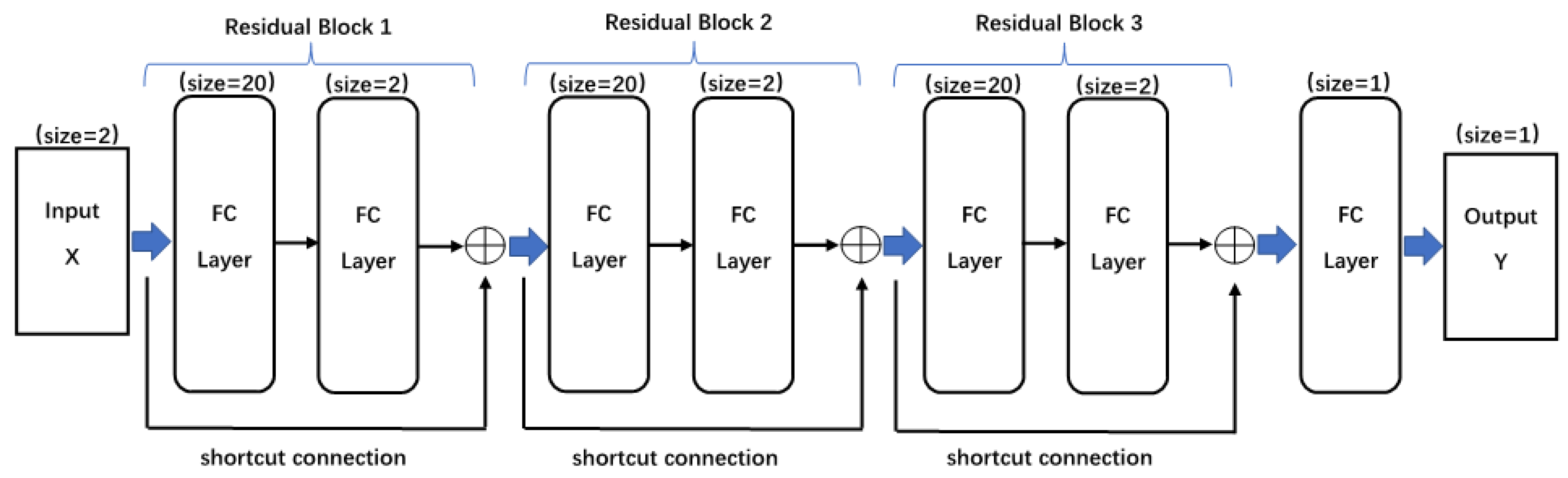
At the end of this section, we describe the structure of DNN used in (28) and (29). The DNN in this paper is a deep residual network (ResNet) [53,64,65] based on the full connection layers. Such a network structure was adopted in [53] to solve the PDEs. The ResNet is an improvement of the conventional DNN. The ResNet can fit high-dimensional functions better, and the fitting ability is not affected by network width. The ResNet can significantly speed training, increase pre-precision, reduce network degradation, and improve network characterization ability.

The ResNet was formally proposed in [64], which is obtained by stacking the residual blocks continuously. Each residual block has consisted of two fully connected layers, and its output is obtained by adding the output of the last layer and the input of the residual block. This structure leads to significant improvement in the training speed and approximation error. Let l be a positive integer. We set that there are l neurons in each layer of ResNet. Let $z_i\in {\mathbb{R}}^l$ be the vector consisted by excitation values of the l neurons in i-th layer, $W_i$ be a $l\times l$ weighted matrix, and $b_i\in {\mathbb{R}}^l$ be a real vector. Furthermore, let $\sigma$ be an activation function. In a ResNet, the vectors $z_{i+1}$ and $z_i$ satisfy

$$z_{i+1}=\sigma (W_i{z}_i+b_i),$$

where $b_i$ is called the bias term. Let ${\phi }_i\left(z\right):=\sigma (W_{i}z+b_i)$, $z\in {\mathbb{R}}^l$. Let $B_j$ be the output of j-th residual block, which satisfies that

$$B_{j+1}:=B_j+{\phi }_{2j}\circ {\phi }_{2j-1}\left(B_j\right).$$

Let ${\psi }_{j+1}\left(z\right):=z+{\phi }_{2j}\circ {\phi }_{2j-1}\left(z\right)$, $z\in {\mathbb{R}}^l$. The relationship between the input X and output Y of the ResNet with N residual blocks is

$$Y={\phi }_{2N+1}\circ {\psi }_N\circ \cdots {\psi }_2\circ {\psi }_1\left(X\right).$$

In our computations, we use a ResNet with three such blocks, see Figure 2. The parameters $W_i$ and $b_i$ for $i\in \{1,2,\dots ,2N+1\}$ are derived by solving the minimization problem (29) based on the loss function (28). These parameters are updated using the back propagation algorithm based on gradients of the loss function with respect to the parameters. In this paper, we use the stochastic gradient descent (SGD) method [66,67] for solving (29). The sigmoid function [62,63] serves as the activation function.

5. Convergence Analysis

We prove the convergence of the SGFEM solution coupled with the DNN, $u_h^{{\theta }_{\ast }}$, in this section. The approximation error of $u_h^{{\theta }_{\ast }}$ involves two parts: the SGFEM error and the learning error of DNN. For any $\vartheta \in {\mathbb{M}}_2$ (see (6)), let

$${\vartheta }_r:=\vartheta {|}_{{\Omega }_r},r=0,1,$$

then ${\vartheta }_r\in H^2\left({\Omega }_r\right),r=0,1$. Since we consider $\mathrm{\Gamma }$ is smooth, ${\vartheta }_0$ and ${\vartheta }_1$ can be continuously extended to the whole domain $\Omega$ to obtain functions ${\tilde{\vartheta }}_0$ and ${\tilde{\vartheta }}_1$ in $H^2(\Omega )$ such that

$${\tilde{\vartheta }}_r={\vartheta }_{r}on{\Omega }_r\mathrm{and}\parallel {\tilde{\vartheta }}_r{\parallel }_{H^2(\Omega )}\le C{\parallel {\vartheta }_r\parallel }_{H^2\left({\Omega }_k\right)},r=0,1,$$

(34)

where C is a positive constant independent of h (see Theorem 1.4.5 in [68]).

Let $\epsilon$ represent the learning error level of ${\tilde{u}}^{{\theta }_{\ast }}$, i.e.,

$$\parallel {\tilde{u}}^{{\theta }_{\ast }}-\tilde{u}{\parallel }_{L^{\infty }\left(\mathrm{\Gamma }\right)}={\parallel {\vartheta }^{{\theta }_{\ast }}-(-\varphi )\parallel }_{L^{\infty }\left(\mathrm{\Gamma }\right)}\le \epsilon .$$

(35)

We first establish a relevant approximation result.

Lemma 1.

Suppose $w\in H^{k+1}\left({\overline{\Omega }}_0\right),k\ge 1$ and ${\parallel w\parallel }_{L^{\infty }\left(\mathrm{\Gamma }\right)}\le \epsilon$, then there is $\widehat{w}\in H^1\left({\overline{\Omega }}_0\right)$ satisfying $\widehat{w}{|}_{\mathrm{\Gamma }}=0$ such that

$$\parallel w-\widehat{w}{\parallel }_{H^1\left({\overline{\Omega }}_0\right)}\le C{\epsilon }^{\frac{k}{k+1}}{\left|w\right|}_{H^{k+1}\left({\overline{\Omega }}_0\right)}^{\frac{1}{k+1}},$$

(36)

where C is a constant independent of ε and k.

Proof. 

We divide ${\Omega }_0$ using a quasi-uniform mesh fitting the interface $\mathrm{\Gamma }$. The mesh-size parameter is denoted by l. We note that such a mesh is used only for obtaining associated estimates, and not used for actual computation. Let $O_j$ and ${\psi }_j$, $j\in {\chi }_l$ be the FE nodes and FE functions of degree k associated with the mesh, respectively, and

$$I_{l}w=\sum _{j\in {\chi }_l}w\left(O_j\right){\psi }_j$$

be the standard FE interpolant of w. The index set ${\chi }_l$ is divided into ${\chi }_l^{\prime }$ and ${\chi }_l^{\prime \prime }$, which consist of indices of nodes on the interface $\mathrm{\Gamma }$ and in the interior of ${\Omega }_0$, respectively. It is easy to know that

$$I_l^{\prime \prime }w:=\sum _{j\in {\chi }_l^{\prime \prime }}w\left(O_j\right){\psi }_j$$

belongs to $H^1\left({\overline{\Omega }}_0\right)$ and satisfies $I_l^{\prime \prime }{w|}_{\mathrm{\Gamma }}=0$. Based on the error estimate of FEM interpolation [68] we have

$$\begin{array}{ccc}\hfill \parallel w-I_l^{\prime \prime }{w\parallel }_{H^1\left({\overline{\Omega }}_0\right)}& \le & \parallel w-I_l{w\parallel }_{H^1\left({\overline{\Omega }}_0\right)}+{∥\sum _{j\in {\chi }_l^{\prime }}w\left(O_j\right){\psi }_j∥}_{H^1\left({\overline{\Omega }}_0\right)}\hfill \\ & \le & C{l}^k{\left|w\right|}_{H^{k+1}\left({\overline{\Omega }}_0\right)}+\sum _{j\in {\chi }_l^{\prime }}|w\left(O_j\right)|\parallel {\psi }_j{\parallel }_{H^1\left({\overline{\Omega }}_0\right)}\hfill \\ & \le & C{l}^k{\left|w\right|}_{H^{k+1}\left({\overline{\Omega }}_0\right)}+\epsilon \sum _{j\in {\chi }_l^{\prime }}{\parallel {\psi }_j\parallel }_{H^1\left({\overline{\Omega }}_0\right)}\hfill \\ & \le & C{l}^k{\left|w\right|}_{H^{k+1}\left({\overline{\Omega }}_0\right)}+\epsilon \sum _{j\in {\chi }_l^{\prime }}{C}^{\prime }\le C{l}^k{\left|w\right|}_{H^{k+1}\left({\overline{\Omega }}_0\right)}+C^{\prime }\epsilon \frac{1}{l},\hfill \end{array}$$

(37)

where the last inequality is because the number of nodes on $\mathrm{\Gamma }$, $|{\chi }_l^{\prime }|$, is $O\left(\frac{1}{l}\right)$. Then letting $l={\left(\frac{\epsilon }{{\left|w\right|}_{H^{k+1}\left({\overline{\Omega }}_0\right)}}\right)}^{\frac{1}{k+1}}$ in (37) yields

$$\begin{array}{c}\hfill \parallel w-I_l^{\prime \prime }{w\parallel }_{H^1\left({\overline{\Omega }}_0\right)}\le C{\epsilon }^{\frac{k}{k+1}}{\left|w\right|}_{H^{k+1}\left({\overline{\Omega }}_0\right)}^{\frac{1}{k+1}}+C^{\prime }{\epsilon }^{\frac{k}{k+1}}{\left|w\right|}_{H^{k+1}\left({\overline{\Omega }}_0\right)}^{\frac{1}{k+1}}\le C{\epsilon }^{\frac{k}{k+1}}{\left|w\right|}_{H^{k+1}\left({\overline{\Omega }}_0\right)}^{\frac{1}{k+1}}.\end{array}$$

(38)

Let $\widehat{w}=I_l^{\prime \prime }w$, then we obtain the desired estimate (36) from (38). □

Theorem 2.

Suppose that $u\in {\mathbb{M}}_2\cap \mathcal{E}(\Omega )$ is the solution to (3)–(5), and $u_h^{{\theta }_{\ast }}:={\tilde{U}}_h^{{\theta }_{\ast }}+{\tilde{u}}^{{\theta }_{\ast }}$ is the SGFEM approximation of u, where $U_h^{{\theta }_{\ast }}$ is the solution of associated CIP (33), and ${\tilde{u}}^{{\theta }_{\ast }}$ is the DNN function (30) that approximates the discontinuous jump ϕ. The learning error level of ${\tilde{u}}^{{\theta }_{\ast }}$ is represented in (35). Let $\tilde{u}$ defined in (20) belongs to $H^{k+1}\left({\overline{\Omega }}_0\right)$. Then there is a constant C that is independent of h, k, and ε such that

$${∥u-u_h^{{\theta }_{\ast }}∥}_{\mathcal{E}(\Omega )}\le Ch{∥{\tilde{U}}^{{\theta }_{\ast }}∥}_{{\mathbb{M}}_2}+C{\epsilon }^{\frac{k}{k+1}}{\left|\tilde{u}-{\tilde{u}}^{{\theta }_{\ast }}\right|}_{H^{k+1}\left({\overline{\Omega }}_0\right)}^{\frac{1}{k+1}},$$

(39)

where ${\tilde{U}}^{{\theta }_{\ast }}$ is defined in (31).

Proof. 

Remembering that $\tilde{U}=u-\tilde{u}$ we have

$$\begin{array}{ccc}\hfill {∥u-u_h^{{\theta }_{\ast }}∥}_{\mathcal{E}(\Omega )}& =& {∥(\tilde{U}+\tilde{u}-{\tilde{U}}^{{\theta }_{\ast }}-{\tilde{u}}^{{\theta }_{\ast }})+({\tilde{U}}^{{\theta }_{\ast }}-{\tilde{U}}_h^{{\theta }_{\ast }})∥}_{\mathcal{E}(\Omega )}\hfill \\ & \le & {∥(\tilde{U}+\tilde{u}-{\tilde{U}}^{{\theta }_{\ast }}-{\tilde{u}}^{{\theta }_{\ast }})∥}_{\mathcal{E}(\Omega )}+{∥U^{{\theta }_{\ast }}-{\tilde{U}}_h^{{\theta }_{\ast }}∥}_{\mathcal{E}(\Omega )}.\hfill \end{array}$$

(40)

According to (26) and (31) we obtain

$$B(\tilde{U}+\tilde{u},V)=B({\tilde{U}}^{{\theta }_{\ast }}+{\tilde{u}}^{{\theta }_{\ast }},V)=0,\forall V\in \mathcal{E}(\Omega ),$$

and thus

$$B(\tilde{U}+\tilde{u}-{\tilde{U}}^{{\theta }_{\ast }}-{\tilde{u}}^{{\theta }_{\ast }},V)=0,\forall V\in \mathcal{E}(\Omega ).$$

Therefore, for arbitrary $V\in \mathcal{E}(\Omega )$

$$\begin{array}{ccc}\hfill {∥\tilde{U}+\tilde{u}-{\tilde{U}}^{{\theta }_{\ast }}-{\tilde{u}}^{{\theta }_{\ast }}∥}_{\mathcal{E}(\Omega )}^2& =& B(\tilde{U}+\tilde{u}-{\tilde{U}}^{{\theta }_{\ast }}-{\tilde{u}}^{{\theta }_{\ast }},\tilde{U}+\tilde{u}-{\tilde{U}}^{{\theta }_{\ast }}-{\tilde{u}}^{{\theta }_{\ast }})\hfill \\ & =& B(\tilde{U}+\tilde{u}-{\tilde{U}}^{{\theta }_{\ast }}-{\tilde{u}}^{{\theta }_{\ast }},\tilde{u}-{\tilde{u}}^{{\theta }_{\ast }}-V)\hfill \\ & \le & {∥\tilde{U}+\tilde{u}-{\tilde{U}}^{{\theta }_{\ast }}-{\tilde{u}}^{{\theta }_{\ast }}∥}_{\mathcal{E}(\Omega )}{∥\tilde{u}-{\tilde{u}}^{{\theta }_{\ast }}-V∥}_{\mathcal{E}(\Omega )}.\hfill \end{array}$$

(41)

Eliminating ${∥\tilde{U}+\tilde{u}-{\tilde{U}}^{{\theta }_{\ast }}-{\tilde{u}}^{{\theta }_{\ast }}∥}_{\mathcal{E}(\Omega )}$ on both sides of (41) we have

$${∥\tilde{U}+\tilde{u}-{\tilde{U}}^{{\theta }_{\ast }}-{\tilde{u}}^{{\theta }_{\ast }}∥}_{\mathcal{E}(\Omega )}\le {∥\tilde{u}-{\tilde{u}}^{{\theta }_{\ast }}-V∥}_{\mathcal{E}(\Omega )},\forall V\in \mathcal{E}(\Omega ).$$

(42)

Let

$$\widehat{V}=\left\{\begin{array}{cc}V,\hfill & \mathrm{in}{\overline{\Omega }}_0,\hfill \\ 0,\hfill & \mathrm{in}{\Omega }_1,\hfill \end{array}\right.$$

which also belongs to $\mathcal{E}(\Omega )$. Hence, we obtain from (42) that

$$\begin{array}{c}\hfill {∥\tilde{U}+\tilde{u}-{\tilde{U}}^{{\theta }_{\ast }}-{\tilde{u}}^{{\theta }_{\ast }}∥}_{\mathcal{E}(\Omega )}\le {∥\tilde{u}-{\tilde{u}}^{{\theta }_{\ast }}-\widehat{V}∥}_{\mathcal{E}(\Omega )}={∥\tilde{u}-{\tilde{u}}^{{\theta }_{\ast }}-\widehat{V}∥}_{\mathcal{E}\left({\overline{\Omega }}_0\right)}\le C{∥\tilde{u}-{\tilde{u}}^{{\theta }_{\ast }}-\widehat{V}∥}_{H^1\left({\overline{\Omega }}_0\right)}.\end{array}$$

(43)

Based on the learning error (35) and Lemma 1, there is a $\widehat{V}$ such that

$${∥\tilde{U}+\tilde{u}-{\tilde{U}}^{{\theta }_{\ast }}-{\tilde{u}}^{{\theta }_{\ast }}∥}_{\mathcal{E}(\Omega )}\le C{\epsilon }^{\frac{k}{k+1}}{\left|\tilde{u}-{\tilde{u}}^{{\theta }_{\ast }}\right|}_{H^{k+1}\left({\overline{\Omega }}_0\right)}^{\frac{1}{k+1}}.$$

(44)

On the other hand, it is noted that ${\tilde{U}}_h^{{\theta }_{\ast }}$ in (33) is the SGFEM solution to the CIP (31). Then according to the approximation result (18) for the CIP in Theorem 1 we have

$${∥{\tilde{U}}^{{\theta }_{\ast }}-{\tilde{U}}_h^{{\theta }_{\ast }}∥}_{\mathcal{E}(\Omega )}\le Ch{∥{\tilde{U}}^{{\theta }_{\ast }}∥}_{{\mathbb{M}}_2}.$$

(45)

Finally, we obtain from the estimates (40), (44), and (45)

$${∥u-u_h^{{\theta }_{\ast }}∥}_{\mathcal{E}(\Omega )}\le Ch{∥{\tilde{U}}^{{\theta }_{\ast }}∥}_{{\mathbb{M}}_2}+C{\epsilon }^{\frac{k}{k+1}}{\left|\tilde{u}-{\tilde{u}}^{{\theta }_{\ast }}\right|}_{H^{k+1}\left({\Omega }_0\right)}^{\frac{1}{k+1}},$$

which is the desired result (39). □

In (39) $\tilde{u}$ only needs the evaluations on $\mathrm{\Gamma }$, i.e., $\tilde{u}{|}_{\mathrm{\Gamma }}=-\varphi$, while its evaluations on ${\Omega }_0$ are not required specifically. Therefore, the term ${\left|\tilde{u}-{\tilde{u}}^{{\theta }_{\ast }}\right|}_{H^{k+1}\left({\Omega }_0\right)}$ in (39) can be replaced by

$$\underset{\tilde{u}\in H^{k+1}\left({\overline{\Omega }}_0\right),\tilde{u}{|}_{\mathrm{\Gamma }}=-\varphi }{min}{\left|\tilde{u}-{\tilde{u}}^{{\theta }_{\ast }}\right|}_{H^{k+1}\left({\Omega }_0\right)},$$

which could be small. In (39) k at least equals to 1, i.e., $\tilde{u}\in H^2\left({\overline{\Omega }}_0\right)$. In fact, let $\tilde{u}{{|}_{{\overline{\Omega }}_0}=[{\tilde{u}}_0-{\tilde{u}}_1]|}_{{\overline{\Omega }}_0}$, where ${\tilde{u}}_0$ and ${\tilde{u}}_1$ are the extensions of $u_0$ and $u_1$ (34), respectively, then $\tilde{u}\in H^2\left({\overline{\Omega }}_0\right)$ and $\tilde{u}{|}_{\mathrm{\Gamma }}=-\varphi$. We mention that for the interface problem where $\mathrm{\Gamma }$ and $\varphi$ are relatively smooth, $\tilde{u}$ could have higher smoothness in ${\overline{\Omega }}_0$, i.e, $\tilde{u}\in H^{k+1}\left({\overline{\Omega }}_0\right),k>1$. Theorem 2 means that the proposed SGFEM coupled with the DNN can obtain the optimal energy error $O\left(h\right)$ if the DNN function ${\tilde{u}}^{{\theta }_{\ast }}$ learns $\tilde{u}$ ($\varphi$) on the interface $\mathrm{\Gamma }$ (not in the domains ${\Omega }_0$ and ${\Omega }_1$) accurately sufficiently, see (35). In the numerical experiments below, the optimal errors $O\left(h\right)$ are observed for the same discretization parameters h as those in the SGFEM for the CIP.

6. Numerical Results

We consider the model problem (3) in a domain $\Omega ={(0,1)}^2$ with straight and curved interfaces $\mathrm{\Gamma }$ for the numerical experiments. We test two cases of coefficients $a\left(P\right)$: (i) $a_0=1$ and $a_1=10$, and (ii) $a_0=1$ and $a_1=100$. Their contrasts are $c=10$ and $c=100$, respectively. The manufactured exact solution u of (3) will be employed in the tests. The loading functions $f,g$ of (3), the jump $\varphi$ (4), and the flux $\psi$ (5) can be calculated by using Equation (3) and the manufactured exact solution u.

The uniform $n\times n$ square FE mesh is used to discretize the domain $\Omega ={(0,1)}^2$ with the mesh parameter $h=1/n$. The nodes associated with the mesh are denoted by ${\left\{P_i\right\}}_{i\in I_h}$, where $I_h$ is the index set. Let ${\left\{{\varphi }_i\right\}}_{i\in I_h}$ be the bilinear FE functions associated with the nodes ${\left\{P_i\right\}}_{i\in I_h}$.

We will test the standard FEM (8) and SGFEM (12) on the square mesh for the DIP, based on the variational formulation (31) incorporating the DNN function (20). We do not present the results of other GFEMs, such as the geometric and corrected GFEM. In the geometric GFEM, the SCN is of order $O\left(h^{-4}\right)$[23], which is much bigger than that of SGFEM. The corrected GFEM is not robust in the sense that the SCN gets bad as interface curves approach boundaries of elements [27]. We compute and compare the relative error of these methods in the energy norm (EE). The SCN of SGFEM has been shown to be of order $O\left(h^{-2}\right)$ in [27], and we do not repeat it in this paper because the stiffness matrices for the DIP are the same as those for the CIP.

Setting for ResNet. As described at the end of Section 4, we use the ResNet for the DNN coupling in the tests. The ResNet structure consists of three residual blocks, each of which contains two full connection layers and one residual item, where each layer contains 20 neurons, see Figure 2. The sigmoid function [62,63] serves as the activation function. We use the stochastic gradient descent (SGD) method [66,67] for solving (29) in the learning process. The learning rate, the batch number, the number $N_{\mathrm{\Gamma }}$ of sampling points on $\mathrm{\Gamma }$ for training the ResNet will be specified in the following Subsections.

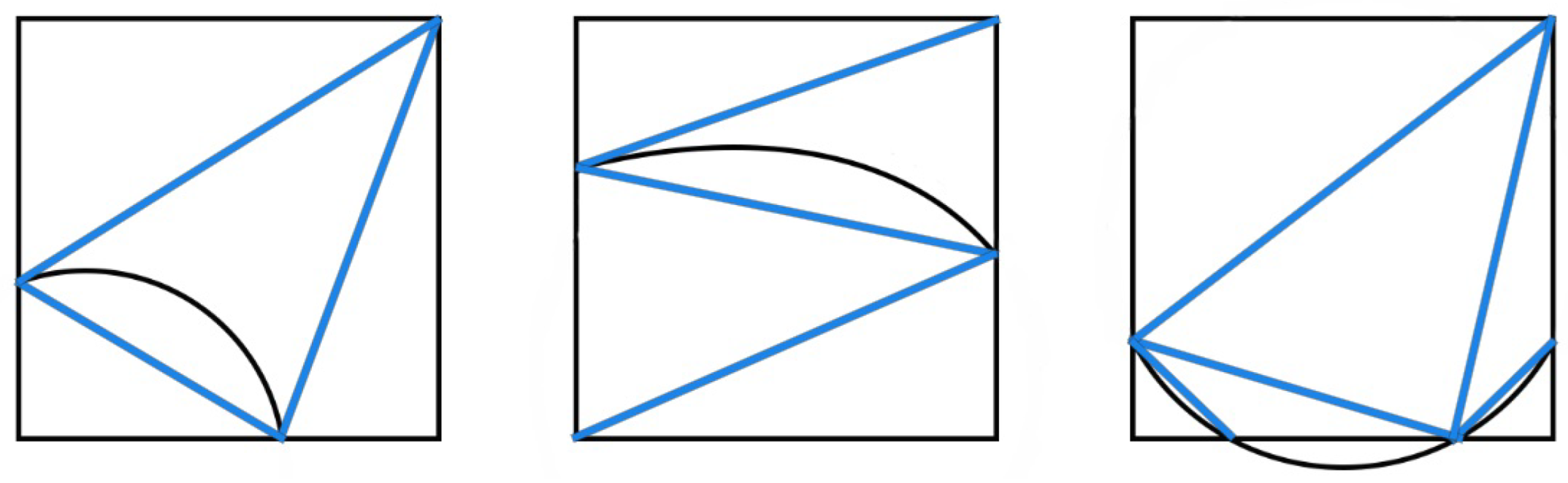
Integration for discontinuous enrichments. We describe the numerical integration formula used in the computations. For elements that do not intersect the interface, we employ the standard $4\times 4$ Gaussian rule. For elements cut by the interface, we connect the intersection points of the interface and the boundaries of an element by a straight line, and decompose the element into 4 to 6 sub-triangles, on each of which the standard 12-point Gaussian rule for triangles is employed. See Figure 3 for an example. We mention that a systematic study of the effect of numerical integration is not the objective of this work. We refer to for more details about the numerical integrations for the interface problems [3,5,22,69].

We now present our numerical results in the following sub-sections.

6.1. A Straight Interface Situation

We first consider a straight interface $\mathrm{\Gamma }$, which has an equation $y=tan\left({\theta }_0\right)(x-1-d)+1$ with ${\theta }_0=\frac{\pi }{6}$ and $d=\frac{1}{\pi }$. The manufactured solution of (3) is as follows:

$$u=\left\{\begin{array}{cc}M{r}^{{\alpha }_0}cos\left({\alpha }_0(\theta +\pi -{\theta }_0)\right)+N\frac{a_0}{a_1}{r}^{{\alpha }_0}sin\left({\alpha }_0(\theta +\pi -{\theta }_0)\right)+sin\left(xy\right),\hfill & y>tan\left({\theta }_0\right)(x-1-d)+1\left({\Omega }_1\right),\hfill \\ r^{{\alpha }_0}cos\left({\alpha }_0(\theta +\pi -{\theta }_0)\right)+r^{{\alpha }_0}sin\left({\alpha }_0(\theta +\pi -{\theta }_0)\right)+sin\left(xy\right),\hfill & y\le tan\left({\theta }_0\right)(x-1-d)+1\left({\Omega }_0\right),\hfill \end{array}\right.$$

where ${\alpha }_0=\frac{4}{3}$, and $(r,\theta )$ is the polar coordinate at the center $(1+d,1)$. It can be checked that u is continuous across the interface $\mathrm{\Gamma }$ when $M=N=1$. In this example we take $M=100$ and $N=100$, and u is discontinuous across $\mathrm{\Gamma }$, i.e., ${\left[u\right]}_{\mathrm{\Gamma }}=\varphi \ne 0$ (see (4)) and also the jump of flux $\psi \ne 0$ (5). The mesh on the domain $[0,1]\times [0,1]$ is refined with $h^{-1}=n=2^{j+1},j=1,2,\cdots ,7$. The interface $\mathrm{\Gamma }$ and a mesh with $n=16$ are shown in Figure 4 Left, and the exact solution u with $a_0=1$ and $a_1=100$ is drawn in Figure 4 Right.

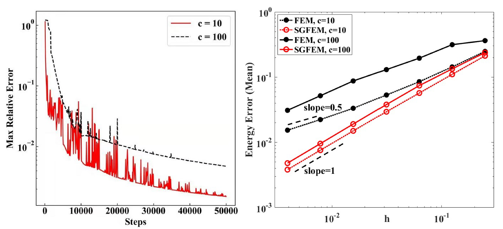
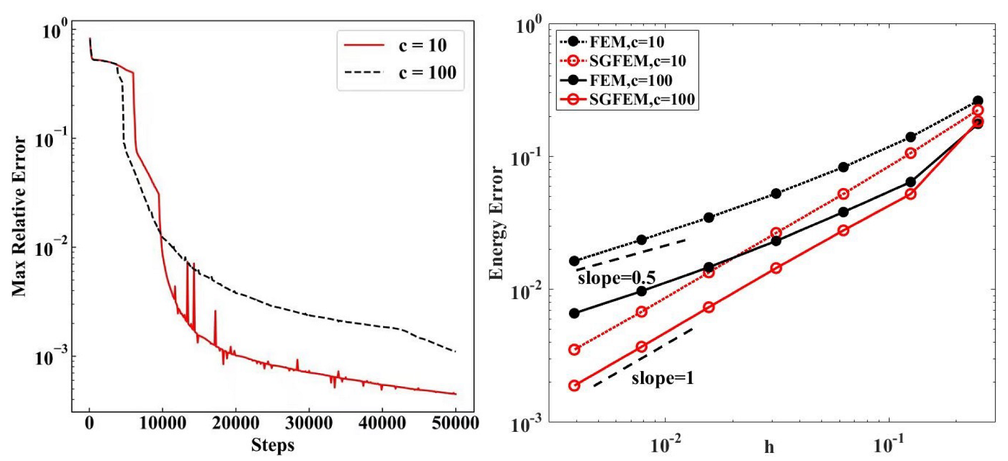
The number of sampling points uniformly for training the ResNet, $N_{\mathrm{\Gamma }}$, is taken as 200 in this situation. The learning rate $\eta =0.05$, and the batch number is 4096. The maximum relative error of DNN function ${\tilde{u}}^{{\theta }_{\ast }}$ (30) to the jump $\varphi$ on $\mathrm{\Gamma }$, defined as

$$\frac{\parallel {\tilde{u}}^{{\theta }_{\ast }}{-\varphi \parallel }_{L^{\infty }\left(\mathrm{\Gamma }\right)}}{{\parallel \varphi \parallel }_{L^{\infty }\left(\mathrm{\Gamma }\right)}},$$

(46)

with respect to the iteration steps of SGD, is shown in Figure 5 Left. It shows that the error of the DNN function ${\tilde{u}}^{{\theta }_{\ast }}$ is reduced by increasing the iteration steps of SGD. We also observed this by testing the different learning rates and batch numbers, and we do not exhibit them here. Therefore, it is easy to learn a DNN function ${\tilde{u}}^{{\theta }_{\ast }}$ to reach the desired error level $\epsilon$ (35) in the Theorem 2 (39). Such an $\epsilon$ is small enough for the SGFEM to obtain the optimal energy error convergence order $O\left(h\right)$, see below for the energy errors.

The energy errors with respect to h of the FEM and SGFEM coupled with the DNN, are presented in Figure 5 Right for different contrasts c (10 and 100), where $h^{-1}=n=2^{j+1},j=1,2,\cdots ,7$. It is shown in Figure 5 Right that the convergence orders of the FEM and SGFEM are $O\left(h^{0.5}\right)$ and $O\left(h\right)$, respectively. Therefore, it is concluded from this set of numerical experiments that the proposed SGFEM reaches the optimal convergence order for such a DIP, as predicted in the Theorem 2 (when $\epsilon$ is small).

6.2. A Curved Interface Situation

We next consider a curved interface $\mathrm{\Gamma }$ with an equation ${(x-x_0)}^2+{(y-y_0)}^2=r_0^2$, where $x_0=\frac{1}{\sqrt{5}},y_0=\frac{1}{\sqrt{3}},r_0=\frac{1}{\sqrt{10}}$. In this case we consider the manufactured solution of (3) as follows:

$$u=\left\{\begin{array}{cc}\frac{2a_1-a_1\rho r_0^2}{(a1-a0)r_0^4}{r}^{2}cos\left(2\theta \right),\hfill & r<r_0\left({\Omega }_0\right),\hfill \\ \frac{a_1+a_0-a_0\rho r_0^2}{(a1-a0)r_0^4}{r}^{2}cos\left(2\theta \right)+r^{-2}cos\left(2\theta \right),\hfill & r\ge r_0\left({\Omega }_1\right),\hfill \end{array}\right.$$

where $(r,\theta )$ is the polar coordinate at the center $(x_0,y_0)$. It can be verified that u is continuous across $\mathrm{\Gamma }$ for $\rho =0$. In this test, we take $\rho =(a_0+a_1)/2$, and ${\left[u\right]}_{\mathrm{\Gamma }}=\varphi$ is non-zero. The interface $\mathrm{\Gamma }$ and a mesh with $n=16$ are shown in Figure 6 Left, and the exact solution u with $a_0=1$ and $a_1=100$ is drawn in Figure 6 Right. The mesh on the domain $[0,1]\times [0,1]$ is refined with $h^{-1}=n=2^{j+1},j=1,2,\cdots ,7$.

The number of sampling points uniformly for training the ResNet, $N_{\mathrm{\Gamma }}$, is taken as 500 in this situation. The learning rate $\eta =0.08$, and the batch number is 4096. The maximum relative error (46) of DNN function ${\tilde{u}}^{{\theta }_{\ast }}$ (30) to the jump $\varphi$ on $\mathrm{\Gamma }$ with respect to the iteration steps of SGD, is shown in Figure 7 Left. It shows that the error of the DNN function is reduced by increasing the iteration steps of SGD. We also observe this by testing the different learning rates and batch numbers, and we do not exhibit them here. Therefore, it is easy to obtain a DNN function ${\tilde{u}}^{{\theta }_{\ast }}$ to reach the small error level $\epsilon$ in the Theorem 2.

We note that the DNN used in this paper is a stochastic method due to the SGD. In this example, to test the robustness of proposed method, we implement the learning algorithm (29) five times to generate the DNN functions ${\tilde{u}}_i^{{\theta }_{\ast }}$ (30), $i=1,2,\cdots ,5$. For each ${\tilde{u}}_i^{{\theta }_{\ast }}$, the energy errors ${EE}_{i,h}$ with respect to h of the coupled FEM and SGFEM are computed from (33). The means and standard deviations (STD) of these errors are defined by

$${\overline{\mathrm{EE}}}_h:=\frac{1}{5}\sum _{i=1}^5{\mathrm{EE}}_{i,h},\mathrm{and}{STD}_h:=\sqrt{\frac{1}{5}{\sum }_{i=1}^5{({EE}_{i,h}-{\overline{EE}}_h)}^2}.$$

${\overline{\mathrm{EE}}}_h$ with respect to h of the FEM and SGFEM are presented in Figure 7 Right for different contrasts c (10 and 100). ${\overline{\mathrm{EE}}}_h$ and ${STD}_h$ with respect to h of SGFEM are listed in

Table 1. The means and STDs of errors with respect to h of SGFEM: the curved interface situation.

h	$\mathit{c}=10$		$\mathit{c}=100$
	Mean	STD	Mean	STD
$2.5000\times {10}^{-01}$	$2.1241\times {10}^{-01}$	$4.0512\times {10}^{-04}$	$2.3789\times {10}^{-01}$	$7.9756\times {10}^{-03}$
$1.2500\times {10}^{-01}$	$1.1036\times {10}^{-01}$	$3.0925\times {10}^{-04}$	$1.3384\times {10}^{-01}$	$8.4100\times {10}^{-03}$
$6.2500\times {10}^{-02}$	$5.7113\times {10}^{-02}$	$1.4862\times {10}^{-04}$	$7.4277\times {10}^{-02}$	$5.5238\times {10}^{-03}$
$3.1250\times {10}^{-02}$	$2.9479\times {10}^{-02}$	$8.1748\times {10}^{-05}$	$3.8006\times {10}^{-02}$	$2.9354\times {10}^{-03}$
$1.5625\times {10}^{-02}$	$1.5016\times {10}^{-02}$	$4.3178\times {10}^{-05}$	$1.9107\times {10}^{-02}$	$1.4815\times {10}^{-03}$
$7.8125\times {10}^{-03}$	$7.5967\times {10}^{-03}$	$2.0323\times {10}^{-05}$	$9.5761\times {10}^{-03}$	$7.4419\times {10}^{-04}$
$3.9063\times {10}^{-03}$	$3.8242\times {10}^{-03}$	$1.0329\times {10}^{-05}$	$4.8098\times {10}^{-03}$	$3.7257\times {10}^{-04}$

.

Figure 7 Right clearly shows that the convergence orders of the error means of FEM and SGFEM are still $O\left(h^{0.5}\right)$ and $O\left(h\right)$, respectively, as predicted. It is observed in Table 1 that the STDs of ${EE}_{i,h}$ are at relatively low levels. These mean that the optimal convergence order, in this case, can also be obtained by the proposed SGFEM, and moreover, the proposed SGFEM exhibits nice robustness with respect to the randomness of the DNN method. We also obtained similar results by testing the different curved interfaces with discontinuous solutions, and we do not present them here.

7. Conclusions and Comments

This paper proposed an SGFEM coupled with the DNN for solving elliptic interface problems with a discontinuous interface condition. In this scheme, the DNN is used to learn a function (approximately) satisfying the interface condition, which helps us formulate the original problems with a discontinuous interface condition into the one with a continuous interface condition. Based on this, the SGFEM for the CIP is applied to the DIP straightforwardly, and no penalty terms are needed. All the merits of SGFEM for the CIP are maintained, such as the optimal convergence, stability, and robustness. The approximation error of the proposed SGFEM coupled with the DNN was analyzed mathematically. For comparison, we performed numerical experiments with the FEM and SGFEM. The FEM converges with an order $O\left(h^{0.5}\right)$ only, while the SGFEM converges with the optimal order $O\left(h\right)$. The proposed method has great potential for the DIP with interfaces of complex geometries due to the meshless features of DNN. The extension of the results in this paper to the three-dimensional and parabolic interface problems will be investigated in future studies.