Using Covering Reduction to Identify Reducts for Object-Oriented Concept Lattices

Abstract

An object-oriented concept lattice, as an important generalization of classic concept lattices, is a bridge between formal concept analysis and rough set theory. This paper presents an application of covering reduction in formal concept analysis. It studies attribute reduction, object reduction, and bireduction for object-oriented concept lattices. We show that attribute and object reductions for object-oriented concept lattices are equivalent to covering reductions. Using a Boolean matrix transformation, we derive the corresponding algorithms to identify all reducts. In contrast to existing discernibility matrix-based reduction algorithms for object-oriented concept lattices, our algorithms omit the calculation of concept lattices, discernibility matrices, and discernibility functions. The algorithms save substantial time and are a significant improvement over discernibility matrix-based techniques.

1. Introduction

Formal concept analysis (FCA) [1,2] is a useful model for the mathematization of concept and conceptual hierarchy. It has become a useful method for knowledge discovery, and the method plays an important role in information retrieval, cognitive analytics, and many other applications. The set of formal concepts may be interpreted as a concept lattice. The lattice has been extensively studied [3,4,5,6,7,8,9], for instance, Aragon, Medina and Poussa [10] studied the impact of applying a local congruence on a concept lattice associated with a reduced context. Particularly, much research has been conducted on attribute reduction for such a lattice [11,12,13,14,15].

Rough set theory (RST) [16,17] serves as an efficient data analysis technique to deal with vagueness and uncertainty. The theory has been extensively used for classification, feature extraction, pattern recognition, and data science. FCA and RST are closely related, for example, object-oriented concept lattices connect FCA and RST. Wei and Qi [18] considered the relationship between FCA and RST. Many papers study concept lattices [19,20,21,22] in FCA by means of rough set approaches. Yao [23,24] gave a comparative study of two theories from a viewpoint of data science. Jose et al. [25] introduced a new attribute reduction method in FCA considering the reduction philosophy given in RST. The method allows to carry out a deeper study of the relation between FCA and RST.

A rough approximation can induce many different lattices, for thorough comprehension of data processing using concept lattices, Gediga and Duntsch [26] introduced attribute-oriented concept lattices (AOCL) based on RST. As a dual concept, Yao [23] defined object-oriented concept lattices (OOCL). Both AOCL and OOCL are important generalizations of the classic concept lattices, they establish the connection between FCA and RST. Generally, a concept lattice may contain superfluous attributes and objects. This leads to the study of attribute or object reduction. The aims of attribute or object reduction for concept lattices are to remove these superfluous attributes or objects. Attribute reduction for concept lattices was proposed by Ganter and Wille [2] and Zhang, Wei, and Qi [27]. According to Konecny [5], the clarification and reduction method can be derived from their book [2]. Zhang, Wei, and Qi [27] used discernibility matrix-based methods to identify all attribute reducts in classic concept lattices. Later, Qi [28] improved their own reduction methods by defining a new discernibility matrix. Using binary integer programming, Li and Zhang [29] proposed a reduction method that does not depend on the discernibility matrices for classic concept lattices.

Attribute reduction is helpful for construction of clear data-based classification and knowledge representation models. It is also a difficult problem in concept lattices. Liu et al. [30] considered the reduction problem of AOCL and OOCL by means of RST. They proposed a discernibility matrix-based reduction algorithm and checked the algorithm by numerical computational results. A discernibility matrix-based algorithm [31] has been standardized for identifying all reducts. The method comes from RST [17] and a similar approach [32] is used to bicluster continuous matrices on the basis of Boolean function analysis. Generally, both concept lattices and discernibility matrices must be calculated. Moreover, a discernibility function must be transformed into its minimal disjunctive normal form. Since it contains several short terms, the method can be used in general; however, it is inefficient and, for large formal contexts, prohibitively costly. For instance, an experimental evaluation by Konecny and Krajča [6] that compared four different reduction algorithms found that the method is inefficient. Shao, Liu, and Guo [33] proposed a Boolean vector-based reduction algorithm that is efficient; however, the algorithm can only identify one reduct rather than all reducts. So we need to set up an efficient reduction algorithm to identify all reducts.

Covering is widely studied in rough sets [34]. Covering reduction is a powerful problem-solving technique, and this paper presents a new covering reduction perspective for solving attribute reduction problems. Fortunately, we have already obtained a simple covering reduction algorithm in [20]. This paper studies the reduction problems in OOCLs and the aim of the paper is to design a simple reduction algorithm to identify all reducts. Specifically, we consider attribute reduction, object reduction and bireduction for OOCLs in formal contexts. We first transform the reduction problem for OOCLs into the reduction problem in coverings and then obtain the corresponding algorithms with the help of the covering reduction algorithm in [20]. All reducts can be directly identified by a Boolean matrix transformation. In particular, our algorithms are simpler than the algorithms given by Liu et al. [30]. This paper can be seen as an application of the covering reduction in reduction theory in formal contexts.

The paper is structured as follows. Section 2 briefly reviews some basic concepts and properties of rough sets, concept lattices and coverings. We show an isomorphic relationship between AOCLs and OOCLs. Section 3 studies the attribute reduction problem for OOCLs and gives an algorithm to identify all reducts with the help of the covering reduction. In Section 4, as a dual of attribute reduction, we consider the object reduction problem in OOCLs and give its reduction algorithm. In Section 5, we discuss the bireduction problem in OOCLs and derive a simple bireduction algorithm. Finally, Section 6 concludes the paper.

2. Preliminaries

We briefly recall basic definitions and properties of rough sets, formal contexts and two types of concept lattices. The detailed definitions can be found in [30]. An isomorphic relationship between AOCLs and OOCLs are established.

We assume that O is a finite object set and A is a finite attribute set. $P\left(O\right)=\left\{P\right|P\subseteq O\}$ is the power set of O. I is called a relation from O to A if $I\subseteq O\times A$. We write $pIq$ for $(p,q)\in I$. A triplet $(O,A,I)$ [2] is called a formal context (for short, context) if I is a relation from O to A. Inverse relation of I is denoted by $I^{-1}$ and $q{I}^{-1}p\iff pIq$. Let $\overline{I}=O\times A-I$ be the complementary relation of I. $\overline{I}$ is also a relation from O to A that can be expressed simple in terms of I: $p\overline{I}q\iff (p,q)\notin I$. Recall that I is called regular [35] if I satisfies, for any $(p,q)\in O\times A$, (1) there exist $q_1,q_2\in A$ such that $(p,q_1)\in I$ and $(p,q_2)\notin I$, and (2) there exist $p_1,p_2\in O$ such that $(p_1,q)\in I$ and $(p_2,q)\notin I$. Clearly, if I is regular, then $I^{-1}$ and $\overline{I}$ are also regular. Suppose $X\times Y\subseteq O\times A$, the restriction of I to $X\times Y$, denoted by $I_{X\times Y}$, is $I\cap (X\times Y)$. Let $p\in O$, the right I-related set of p is

$$r_I\left(p\right)=\left\{q\right|q\in A,pIq\}.$$

Similarly, for $q\in A$, the left I-related set of q is

$$l_I\left(q\right)=\left\{p\right|p\in O,pIq\}.$$

Clearly, for $p\in O$, $l_{I^{-1}}\left(p\right)=r_I\left(p\right)$ and for $q\in A$, $r_{I^{-1}}\left(q\right)=l_I\left(q\right)$. The lower and upper approximations $\underline{I},\overline{I}:P\left(A\right)\to P\left(O\right)$ is given by [36], $Q\subseteq A$

$$\underline{I}\left(Q\right)=\left\{p\right|p\in O,r_I\left(p\right)\subseteq Q\},$$

$$\overline{I}\left(Q\right)=\left\{p\right|p\in O,r_I\left(p\right)\cap Q\ne \varnothing \}$$

respectively. Because $I^{-1}$ is a relation from A to O, for $P\in P\left(O\right)$, using $I^{-1}$ instead of I, we also have the lower and upper approximations $\underline{I^{-1}}\left(P\right)$ and $\overline{I^{-1}}\left(P\right)$. Let $P\subseteq O$, we denote [23]

$$P^{\square }=\underline{I^{-1}}\left(P\right)\mathrm{and}{P}^{◊}=\overline{I^{-1}}\left(P\right),$$

respectively. Similarly, for $Q\subseteq A$, we denote [23]

$$Q^{\square }=\underline{I}\left(Q\right)\mathrm{and}{Q}^{◊}=\overline{I}\left(Q\right).$$

Proposition 1

([23,30]). Let S be a context,

(1) $P^{\square ◊}\subseteq P\subseteq P^{◊\square }$ for $P\in P\left(O\right)$ and $Q^{\square ◊}\subseteq Q\subseteq Q^{◊\square }$ for $Q\in P\left(A\right)$.

(2) $P^{\square ◊\square }=P^{\square }$ and $P^{◊\square ◊}=P^{◊}$ for $P\in P\left(O\right)$. Similarly, $Q^{\square ◊\square }=Q^{\square }$ and $Q^{◊\square ◊}=Q^{◊}$ for $Q\in P\left(A\right)$.

Definition 1

([2,23,27]). Let S be a context.

(1) Assume that $\mathbb{O}(O,A,I)=\left\{(P,Q)\right|P\in P\left(O\right),Q\in P\left(A\right),P^{\square }=Q,Q^{◊}=P\}$, define the meet and join operations on $\mathbb{O}(O,A,I)$ as follows.

$$(P_1,Q_1)\wedge (P_2,Q_2)=({(P_1\cap P_2)}^{\square ◊},Q_1\cap Q_2),and$$

$$(P_1,Q_1)\vee (P_2,Q_2)=(P_1\cup P_2,{(Q_1\cup Q_2)}^{◊\square }),$$

respectively.

(2) Assume that $\mathbb{A}(O,A,I)=\left\{(P,Q)\right|P\in P\left(O\right),Q\in P\left(A\right),P^{◊}=Q,Q^{\square }=P\}$, define the meet and join operations on $\mathbb{A}(O,A,I)$ as follows.

$$(P_1,Q_1)\wedge (P_2,Q_2)=(P_1\cap P_2,{(Q_1\cap Q_2)}^{\square ◊},and$$

$$(P_1,Q_1)\vee (P_2,Q_2)=({(P_1\cup P_2)}^{◊\square },Q_1\cup Q_2),$$

respectively.

$\left(\mathbb{O}\right(O,A,I),\wedge ,\vee )$ is a lattice [2,23,27] and called the object-oriented concept lattice (OOCL) of S. Similarly, $\left(\mathbb{A}\right(O,A,I),\wedge ,\vee )$ is also a lattice and called the attribute-oriented concept lattice (AOCL) of S. As Yao points out in [23], the OOCL and AOCL of S are anti-isomorphic. The following theorem reflects the isomorphic relationship between $\mathbb{A}(O,A,I)$ and $\mathbb{O}(A,O,I^{-1})$.

Theorem 1

([30]). Let S be a context.

(1) $(P,Q)\in \mathbb{A}(O,A,I)\iff (Q,P)\in \mathbb{O}(A,O,I^{-1})$.

(2) $\mathbb{A}(O,A,I)$ is isomorphic to $\mathbb{O}(A,O,I^{-1})$.

By Theorem 1, the reduction problems in AOCLs can be transformed into the reduction problems in OOCLs. Thus, we only consider the reduction problems in OOCLs. We denote

$${\mathbb{O}}_{\mathrm{L}}(O,A,I)=\left\{P\right|P\subseteq O,\exists Q\subseteq A,(P,Q)\in \mathbb{O}(O,A,I)\},\mathrm{and}$$

$${\mathbb{O}}_{\mathrm{R}}(O,A,I)=\left\{Q\right|Q\subseteq A,\exists P\subseteq O,(P,Q)\in \mathbb{O}(O,A,I)\}.$$

$({\mathbb{O}}_{\mathrm{L}}(O,A,I),\wedge ,\vee )$ is a lattice, its meet and join operations are given by

$$P_1\wedge P_2={(P_1\cap P_2)}^{\square ◊}\mathrm{and}{P}_1\vee P_2=P_1\cup P_2\mathrm{for}{P}_1,P_2\in {\mathbb{O}}_{\mathrm{L}}(O,A,I),$$

respectively. Clearly, ${\mathrm{l}}_I\left(p\right)\in {\mathbb{O}}_{\mathrm{L}}(O,A,I)$ for each $p\in A$ and each set of ${\mathbb{O}}_{\mathrm{L}}(O,A,I)$ is a union of some ${\mathrm{l}}_I\left(p\right),p\in A$.

Similarly, $({\mathbb{O}}_{\mathrm{R}}(O,A,I),\wedge ,\vee )$ is also a lattice, and its meet and join operations are

$$Q_1\wedge Q_2=Q_1\cap Q_2\mathrm{and}{Q}_1\vee Q_2={(Q_1\cup Q_2)}^{◊\square }\mathrm{for}{Q}_1,Q_2\in {\mathbb{O}}_{\mathrm{R}}(O,A,I),$$

respectively.

Theorem 2.

Let S be a context, three lattices $\mathbb{O}(O,A,I)$, ${\mathbb{O}}_{\mathrm{L}}(O,A,I)$ and ${\mathbb{O}}_{\mathrm{R}}(O,A,I)$ are isomorphic.

Definition 2.

Let S be a context. S is row clarified if $p_1\ne p_2$ implies ${\mathrm{r}}_I\left(p_1\right)\ne {\mathrm{r}}_I\left(p_2\right)$ for each $p_1,p_2\in O$; S is column clarified if $q_1\ne q_2$ implies ${\mathrm{l}}_I\left(q_1\right)\ne {\mathrm{l}}_I\left(q_2\right)$ for each $q_1,q_2\in A$; S is clarified [2] if S is row and column clarified.

Clearly, in a row clarified context, different objects have different intents, similarly, in a column clarified context, different attributes have different extents. The clarification process is as below. Let $S=(O,A,I)$ be a context, we define an equivalence relation ${\alpha }_I$ on A as follows. $q_1{\alpha }_I{q}_2\iff {\mathrm{l}}_I\left(q_1\right)={\mathrm{l}}_I\left(q_2\right)$ for $q_1,q_2\in A$. The equivalence class containing q is denoted by $\left[q\right]$ and the corresponding quotient set is denoted by $A/{\alpha }_I$. This induces a relation $I_{\alpha }$ from O to $A/{\alpha }_I$ as follows. $p\in O,q\in A,p{I}_{\alpha }\left[q\right]\iff pIt$ for some $t\in \left[q\right]$. It is easy to check that $(O,A/{\alpha }_I,I_{\alpha })$ is a column clarified context. Similarly, if we define an equivalence relation ${\beta }_I$ on O as follows. $p_1{\beta }_I{p}_2\iff {\mathrm{r}}_I\left(p_1\right)={\mathrm{r}}_I\left(p_2\right)$ for $p_1,p_2\in O$. Let $\left[p\right]$ denote the equivalence class containing $p\in O$ and $O/{\beta }_I$ denote the corresponding quotient set, a relation $I_{\beta }$ from $O/{\beta }_I$ to A is given by $p\in O,q\in A,\left[p\right]I_{\beta }q\iff sIq$ for some $s\in \left[p\right]$. Then, $(O/{\beta }_I,A,I_{\beta })$ is a row clarified context. Using similar techniques, we can construct a clarified context $(O/{\beta }_I,A/{\alpha }_I,I_{\alpha ,\beta })$.

Example 1.

Let a context S be given in

Table 1. A formal context.

I	${\mathit{q}}_1$	${\mathit{q}}_2$	${\mathit{q}}_3$	${\mathit{q}}_4$	${\mathit{q}}_5$	${\mathit{q}}_6$	${\mathit{q}}_7$
$p_1$	*		*	*	*	*	*
$p_2$		*	*		*	*	*
$p_3$	*			*	*	*	*
$p_4$		*			*
$p_5$		*			*
$p_6$			*			*	*

, where $O=\{p_1,p_2,p_3,p_4,p_5,p_6\}$ is the object set and $A=\{q_1,q_2,q_3,q_4,q_5,q_6,q_7\}$ is the attribute set. A star * in $(i,j)$ position of the table means that the object $p_i$ has the attribute $q_j$. That is, $p_{i}I{q}_j$. By direct computation, ${\mathrm{l}}_I\left(q_1\right)={\mathrm{l}}_I\left(q_4\right)=\{p_1,p_3\},{\mathrm{l}}_I\left(q_2\right)=\{p_2,p_4,p_5\},{\mathrm{l}}_I\left(q_3\right)=\{p_1,p_2,p_6\}$, ${\mathrm{l}}_I\left(q_5\right)=\{p_1,p_2,p_3,p_4,p_5\}$ and ${\mathrm{l}}_I\left(q_6\right)=l_I\left(q_7\right)=\{p_1,p_2,p_3,p_6\}$. Thus $A/{\alpha }_I=\{\left[q_1\right],\left[q_2\right],\left[q_3\right],\left[q_5\right]$, $\left[q_6\right]\}$, where $\left[q_1\right]=\{q_1,q_4\}=\left[q_4\right]$ and $\left[q_6\right]=\{q_6,q_7\}=\left[q_7\right]$.

1. The column clarified context $(O,A/{\alpha }_I,I_{\alpha })$ is given as in

Table 2. A column clarified context.

${\mathit{I}}_{\mathit{\alpha }}$	$\left[{\mathit{q}}_1\right]=\left[{\mathit{q}}_4\right]$	$\left[{\mathit{q}}_2\right]$	$\left[{\mathit{q}}_3\right]$	$\left[{\mathit{q}}_5\right]$	$\left[{\mathit{q}}_6\right]=\left[{\mathit{q}}_7\right]$
$p_1$	*		*	*	*
$p_2$		*	*	*	*
$p_3$	*			*	*
$p_4$		*		*
$p_5$		*		*
$p_6$			*		*

.

2. The row clarified context $(O/{\beta }_I,A,I_{\beta })$ is given as in

Table 3. A row clarified context.

${\mathit{I}}_{\mathit{\beta }}$	${\mathit{q}}_1$	${\mathit{q}}_2$	${\mathit{q}}_3$	${\mathit{q}}_4$	${\mathit{q}}_5$	${\mathit{q}}_6$	${\mathit{q}}_7$
$\left[p_1\right]$	*		*	*	*	*	*
$\left[p_2\right]$		*	*		*	*	*
$\left[p_3\right]$	*			*	*	*	*
$\left[p_4\right]=\left[p_5\right]$		*			*
$\left[p_6\right]$			*			*	*

.

3. The clarified context $(O/{\beta }_I,A/{\alpha }_I,I_{\beta ,\alpha })$ is given as in

Table 4. A clarified context.

${\mathit{I}}_{\mathit{\alpha },\mathit{\beta }}$	$\left[{\mathit{q}}_1\right]=\left[{\mathit{q}}_4\right]$	$\left[{\mathit{q}}_2\right]$	$\left[{\mathit{q}}_3\right]$	$\left[{\mathit{q}}_5\right]$	$\left[{\mathit{q}}_6\right]=\left[{\mathit{q}}_7\right]$
$\left[p_1\right]$	*		*	*	*
$\left[p_2\right]$		*	*	*	*
$\left[p_3\right]$	*			*	*
$\left[p_4\right]=\left[p_5\right]$		*		*
$\left[p_6\right]$			*		*

.

Definition 3

([34]). A covering Γ of O is a family of nonempty subsets of O such that ${\bigcup }_{X\in \Gamma }X=O$. Assume $Z\in \Gamma$, Z is called reducible if $\exists \varnothing \ne {\Gamma }^{\prime }\subseteq \Gamma$ such that $Z\notin {\Gamma }^{\prime }$ and $Z={\bigcup }_{X\in {\Gamma }^{\prime }}X$; otherwise, Z is irreducible. If ${\Gamma }^{\prime }\subseteq \Gamma$, ${\Gamma }^{\prime }$ is a covering of O and ${\Gamma }^{\prime }$ consists of irreducible elements in Γ, then ${\Gamma }^{\prime }$ is called a reduct of Γ. Each covering has a unique reduct [34].

Coverings and column clarified contexts are closely related. Let $O=\{p_1,p_2$, $\dots ,p_n\}$, if $\Gamma =\{K_1,K_2,\dots ,K_m\}$ is a covering of O, we define $A=\{q_1,q_2,\dots ,q_m\}$ and a relation I from O to A via ${\mathrm{l}}_I\left(q_i\right)=K_i$ for $i\in \{1,2,\dots ,m\}$. Clearly, $(O,A,I)$ is a column clarified context. Conversely, $(O,A,I)$ is a column clarified context with ${\mathrm{l}}_I\left(a\right)\ne \varnothing$ for $a\in A$, then $\left\{{\mathrm{l}}_I\left(a\right)\right|a\in A\}$ is a covering of ${\bigcup }_{a\in A}{\mathrm{l}}_I\left(a\right)$. We [20] proposed a covering reduction algorithm to identify the reduct. We will use the covering reduction algorithm [20] to identify all reducts for OOCLs.

3. Attribute Reduction in Object-Oriented Concept Lattices

Liu et al. [30] considered attribute reduction for OOCLs in contexts. We continue to consider the same reduction problem and provide an attribute reduction algorithm for such a concept lattice in contexts. However, our algorithm is much simpler than that of Liu et al. [30]. In fact, this is an application of covering reduction to attribute reduction in OOCLs. The following are the definitions of attribute and object reductions for OOCLs.

Definition 4

([27]). Let S be a context and B be a nonempty subset of A. If B satisfies the following axioms:

(1) $\mathbb{O}(O,A,I)\cong \mathbb{O}(O,B,I_{O\times B})$ (lattice isomorphism), and 

(2) $\varnothing \ne C\subset B$, $\mathbb{O}(O,A,I)$ is not lattice isomorphic to $\mathbb{O}(O,C,I_{O\times C})$.

Then, B is called an attribute reduct of S.

Note that in Definition 4, (1) guarantees that $\mathbb{O}(O,A,I)$ is invariant under lattice isomorphism and (2) requires B to be minimal.

Definition 5.

Let S be a context and V be a nonempty subset of O. If V satisfies the following axioms:

(1) $\mathbb{O}(O,A,I)\cong \mathbb{O}(V,A,I_{V\times A})$ (lattice isomorphism), and 

(2) for $\varnothing \ne W\subset V$, $\mathbb{O}(O,A,I)$ is not lattice isomorphic to $\mathbb{O}(W,A,I_{W\times A})$.

Then V is called an object reduct of S.

Similarly, in Definition 5, (1) guarantees that $\mathbb{O}(O,A,I)$ is invariant under lattice isomorphism and (2) requires V to be minimal. For an AOCL, we can define the attribute and object reductions, respectively. Let $E\subseteq P\left(O\right)$, we use Span$\left(E\right)$ to denote the family spanned by E, that is, each element in Span$\left(E\right)$ can be written as a union of subsets in E. For example, if $O=\{1,2,3,4\}$ and $E=\left\{\right\{1,2\},\{1,3\left\}\right\}$, then Span$\left(E\right)=\{\varnothing ,\{1,2\},\{1,3\},\{1,2,3\left\}\right\}$. Recall that each covering [34] has a unique reduct. We obtained a covering reduction algorithm in [20].

Theorem 3.

Let S be a context and C be a nonempty subset of A.

(1) For $q\in A$, $({\mathrm{l}}_I\left(q\right),{\mathrm{l}}_I{\left(q\right)}^{\square })\in \mathbb{O}(O,A,I)$.

(2) For $Q\subseteq A$, $(\overline{I}\left(Q\right),\overline{I}{\left(Q\right)}^{\square })\in \mathbb{O}(O,A,I)$.

(3) $\mathbb{O}(O,A,I)\cong \mathbb{O}(O,C,I_{O\times C})$ if and only if Span$\left(\left\{{\mathrm{l}}_I\left(q\right)\right|q\in A\}\right)$=Span$\left(\left\{{\mathrm{l}}_I\left(q\right)\right|q\in C\}\right)$.

(4) Let S be column clarified, C is an attribute reduct of S if and only if $\left\{{\mathrm{l}}_I\left(q\right)\right|q\in C\}$ is a covering reduct of $\left\{{\mathrm{l}}_I\left(q\right)\right|q\in A\}$. In particular, S has a unique attribute reduct.

Proof. 

(1) For $q\in A$, $\overline{I}\left(\left\{q\right\}\right)={\mathrm{l}}_I\left(q\right)={\left\{q\right\}}^{◊}$, $({\left\{q\right\}}^{◊},{\left\{q\right\}}^{◊\square })=({\mathrm{l}}_I\left(q\right),{\mathrm{l}}_I{\left(q\right)}^{\square })\in \mathbb{O}(O,A,I)$.

(2) $\overline{I}\left(Q\right)={\bigcup }_{q\in Q}{\mathrm{l}}_I\left(q\right)$, by part (1),

$(\overline{I}\left(Q\right),\overline{I}{\left(Q\right)}^{\square })=({\bigcup }_{q\in Q}{\mathrm{l}}_I\left(q\right),\overline{I}{\left(Q\right)}^{\square })$$={\bigvee }_{a\in Q}({\mathrm{l}}_I\left(q\right),{\mathrm{l}}_I{\left(q\right)}^{\square })\in \mathbb{O}(O,A,I)$.

(3) Suppose that $(P,Q)\in \mathbb{O}(O,A,I)$, then $P=\overline{I}\left(Q\right)={\bigcup }_{q\in Q}{\mathrm{l}}_I\left(q\right)$. Thus, ${\mathbb{O}}_{\mathrm{L}}(O,A,I)$ and ${\mathbb{O}}_{\mathrm{L}}(O,C,I)$ are spanned by $\left\{{\mathrm{l}}_I\left(q\right)\right|q\in A\}$ and $\left\{{\mathrm{l}}_I\left(q\right)\right|q\in C\}$, respectively. Hence,

$$\mathbb{O}(O,A,I)\cong \mathbb{O}(O,C,I_{O\times B})$$

$$\iff {\mathbb{O}}_{\mathrm{L}}(O,A,I)={\mathbb{O}}_{\mathrm{L}}(O,C,I)$$

$$\iff \mathrm{Span}\left(\left\{{\mathrm{l}}_I\left(q\right)\right|q\in A\}\right)=\mathrm{Span}\left(\left\{{\mathrm{l}}_I\left(q\right)\right|q\in C\}\right).$$

This proves the theorem.

(4) $\left\{{\mathrm{l}}_I\left(q\right)\right|q\in A\}$ is always a covering of ${\bigcup }_{q\in A}{\mathrm{l}}_I\left(q\right)$. In this situation, C is an attribute reduct of S, then $\left\{{\mathrm{l}}_I\left(q\right)\right|q\in C\}$ is a covering reduct of $\left\{{\mathrm{l}}_I\left(q\right)\right|q\in A\}$ and vice versa. S has a unique attribute reduct because each covering has unique reducts.    □

We always have ${\mathbb{O}}_{\mathrm{L}}(O,A,I)=\mathrm{Span}\left(\left\{{\mathrm{l}}_I\left(q\right)\right|q\in A\}\right)$ for any context S. For a column clarified context, by Theorem 3, to identify an attribute reduct of S is equivalent to identifying the covering reduct of $\left\{{\mathrm{l}}_I\left(q\right)\right|q\in A\}$. If S is not column clarified, we use a column clarified context $(O,A/{\alpha }_I,I_{\alpha })$ to replace $(O,A,I)$. Let $\{\left[q_{j_1}\right],\left[q_{j_2}\right],\dots ,\left[q_{j_t}\right]\}$ be the unique attribute reduct of $(O,A/{\alpha }_I,I_{\alpha })$, then each attribute reduct of $(O,A,I)$ has the form $\{q_{i_1},q_{i_2},\dots ,q_{i_t}|q_{i_l}\in \left[q_{j_l}\right],l\in \{1,2,\dots ,t\}\}$. Thus, there are $|\left[q_{j_1}\right]\left|\right|\left[q_{j_2}\right]|\dots |\left[q_{j_t}\right]|$ different attribute reducts, where $\left|X\right|$ is the cardinality of X. Therefore, we only need to give a reduction algorithm for column clarified contexts.

Let $S=(O,A,I)$ be column clarified, where $O=\{p_1,p_2,\dots ,p_m\}$ and $A=\{q_1,q_2,\dots$, $q_n\}$. $M_I$ is the relation matrix of I. Suppose that $\left\{{\mathrm{l}}_I\left(q\right)\right|q\in A\}=\{{\mathrm{l}}_I\left(q_1\right),{\mathrm{l}}_I\left(q_2\right),\dots ,{\mathrm{l}}_I\left(q_n\right)\}$ and $|{\mathrm{l}}_I\left(q_i\right)|\le |{\mathrm{l}}_I\left(q_j\right)|$ for $i<j$. By characteristic function of sets, we write ${\mathrm{l}}_I\left(q_i\right)$ as an n-Boolean column vector ${(a_{1i},a_{2i},\dots ,a_{mi})}^{\mathrm{T}}$ and Boolean matrix $W=(l_I\left(q_1\right),l_I\left(q_2\right),\dots ,l_I\left(q_n\right))$, where $\mathrm{T}$ is transpose. A combination of Theorem 3 and the covering reduction algorithm [20] derives the following Algorithm 1.

Algorithm 1: An attribute reduction algorithm for OOCL.

Input: A column clarified context S. Output: A unique attribute reduct of S. 1. For $i=1$ to $n-1$       a. For $j=i+1$ to n          1. If ${\mathrm{l}}_I\left(q_i\right)\subseteq {\mathrm{l}}_I\left(q_j\right)$, then $-1$ times the ith column is added to the jth column. That is, ${(-a_{1i},-a_{2i},\dots ,-a_{mi})}^T$ is added to ${(a_{1j},a_{2j},\dots ,a_{mj})}^T$ (denoted by $C_j-C_i)$. The family of all attributes, whose columns contain at least one 1, forms the reduct.

Algorithm 1 follows from Theorem 3(4) and the reduction algorithm of coverings [20]. We now analyze the number of steps required by Algorithm 1. We require n steps to finish the calculation of the last step in Algorithm 1; thus, this algorithm requires at most $\left(\right(m-1)+(m-2)+\dots +2+1)n=0.5m(m-1)n$ steps. Hence, its computational complexity is $\mathrm{O}\left(0.5m(m-1)n\right)=\mathrm{O}\left(n{m}^2\right)$.

If we compare with the existing reduction algorithm in [30], the advantages of our algorithm are as follows.

(1) Omit the computation of $\mathbb{O}(O,A,I)$.

(2) Omit the calculation of discernibility matrix and discernibility function.

As we know, the computation of $\mathbb{O}(O,A,I)$, discernibility matrix and discernibility function are difficult and time-consuming. Our reduction algorithms save substantial time and are a significant improvement over discernibility matrix-based techniques. Compared with the clarification and reduction method [6], our algorithms are also more intuitive and easy to understand. We present its reduction algorithm via the following example.

Example 2.

Let a context S be given in Example 1, S is not column clarified. Now we identify the unique reduct of covering $\{{\mathrm{l}}_I\left(q_1\right)(={\mathrm{l}}_I\left(q_4\right)),{\mathrm{l}}_I\left(q_2\right),{\mathrm{l}}_I\left(q_3\right),{\mathrm{l}}_I\left(q_5\right),{\mathrm{l}}_I\left(q_6\right)(={\mathrm{l}}_I\left(q_7\right))\}$ of O by our algorithm.

Step 1. We obtain a column clarified context and construct a Boolean matrix W.

$\left(\begin{array}{cccccc}& q_{1,4}& q_2& q_3& q_5& q_{6,7}\\ p_1& 1& & 1& 1& 1\\ p_2& & 1& 1& 1& 1\\ p_3& 1& & & 1& 1\\ p_4& & 1& & 1& \\ p_5& & 1& & 1& \\ p_6& & & 1& & 1\end{array}\right)$, where $q_{1,4}=\{q_1,q_4\}$ and $q_{6,7}=\{q_6,q_7\}$.

Step 2. According to Algorithm 1, we do the column transformation for W.

$\left(\begin{array}{ccccc}1& & 1& 1& 1\\ & 1& 1& 1& 1\\ 1& & & 1& 1\\ & 1& & 1& \\ & 1& & 1& \\ & & 1& & 1\end{array}\right)$$\overrightarrow{\frac{C_4-C_1}{C_5-C_1}}$$\left(\begin{array}{ccccc}1& & 1& 0& 0\\ & 1& 1& 1& 1\\ 1& & & 0& 0\\ & 1& & 1& \\ & 1& & 1& \\ & & 1& & 1\end{array}\right)$$\overrightarrow{C_4-C_2}$

$\left(\begin{array}{ccccc}1& & 1& 0& 0\\ & 1& 1& 0& 1\\ 1& & & 0& 0\\ & 1& & 0& \\ & 1& & 0& \\ & & 1& & 1\end{array}\right)$$\overrightarrow{C_5-C_3}$$\left(\begin{array}{ccccc}1& & 1& 0& -1\\ & 1& 1& 0& 0\\ 1& & & 0& 0\\ & 1& & 0& \\ & 1& & 0& \\ & & 1& & 0\end{array}\right)$, where$C_j-C_i$means that$-1$multiplying the ith column is added to the jth column.

Step 3. Obtain all reducts.

$\{{\mathrm{l}}_I\left(q_1\right)(={\mathrm{l}}_I\left(q_4\right)),{\mathrm{l}}_I\left(q_2\right),{\mathrm{l}}_I\left(q_3\right)\}$ is the unique reduct of covering $\left\{{\mathrm{l}}_I\left(q\right)\right|q\in A\}$ of O. Since $\left|\right[q_1\left]\right|=2$, $\left|\right[q_2\left]\right|=1$ and $\left|\right[q_3\left]\right|=1$, there are two different attribute reducts. Hence, $\{q_1,q_2,q_3\}$ and $\{q_2,q_3,q_4\}$ are all attribute reducts of S.

In fact, $\mathbb{O}(O,A,I)=$ $\{(\varnothing ,\varnothing ),(p_1{p}_3,q_1{q}_4),(p_2{p}_4{p}_5,q_2),(p_1{p}_2{p}_6,q_3),(p_1{p}_2{p}_3{p}_4{p}_5,$ $q_1{q}_2{q}_4{q}_5),(p_1{p}_2{p}_3{p}_6,q_1{q}_3{q}_4{q}_6),(p_1{p}_2{p}_4{p}_5{p}_6,q_2{q}_3),(O,A)\left\}\right\}.$ Figure 1 shows the Hasse diagram of $\mathbb{O}(O,A,I)$.

By Theorem 1, we can induce an object reduction algorithm for $\mathbb{A}(O,A,I)$.

Corollary 1.

Let S be a context and V be a nonempty subset of O, then $\mathbb{A}(O,A,I)\cong \mathbb{A}(V,A,I_{V\times A})$ if and only if Span$\left\{{\mathrm{r}}_I\left(p\right)\right|p\in O\}=Span\left\{{\mathrm{r}}_I\left(p\right)\right|p\in V\}$. In particular, V is an object reduct for $\mathbb{A}(O,A,I)$ if and only if $\left\{{\mathrm{r}}_I\left(p\right)\right|p\in V\}$ is a covering reduct of $\left\{{\mathrm{r}}_I\left(y\right)\right|y\in O\}$. Moreover, if S is row clarified, then S has a unique object reduct.

Proof. 

By duality principle, the proof is straightforward. □

Example 3.

Let S be given in Example 1, $C=\left\{{\mathrm{r}}_I\left(p\right)\right|p\in O\}=\{\{q_1,q_3,q_4,q_5,q_6,q_7\},\{q_2,q_3,$$q_5,q_6,q_7\},\{q_1,q_4,q_5,q_6,q_7\},\{q_2,q_5\},\{q_3,q_6,q_7\}\}$. C is a covering of A. $\{{\mathrm{r}}_I\left(p_3\right)=\{q_1,q_4,q_5,$$q_6,q_7\},{\mathrm{r}}_I\left(p_4\right)={\mathrm{r}}_I\left(p_5\right)=\{q_2,q_5\},{\mathrm{r}}_I\left(p_6\right)=\{q_3,q_6,q_7\}\}$ is the unique reduct of C. Thus, $\{p_3,p_4,p_6\}$ and $\{p_3,p_5,p_6\}$ are all object reducts for $\mathbb{A}(O,A,I)$.

4. Object Reduction in Object-Oriented Concept Lattices

The dual concept of attribute reduction is object reduction. We will set up an object reduction algorithm for OOCLs. Let A be a finite set and $F\subseteq P\left(A\right)$, we denote $F^{\prime }=\left\{P\right|A-P\in F\}$ and $P^{\prime }=A-P$ for $P\subseteq A$.

Theorem 4.

Let S be a context and V be a nonempty subset of O, then:

(1) For each $p\in O$, $({\left({\mathrm{r}}_I^{\prime }\left(p\right)\right)}^{◊},{\mathrm{r}}_I^{\prime }\left(p\right))\in \mathbb{O}(O,A,I)$.

(2) $\mathbb{O}(O,A,I)\cong \mathbb{O}(V,A,I_{V\times A})$ if and only if Span$\left\{{\mathrm{r}}_I\left(p\right)\right|p\in O\}=Span\left\{{\mathrm{r}}_I\left(p\right)\right|p\in V\}$.

(3) Let S be row clarified, then V is an object reduct of S if and only if $\left\{{\mathrm{r}}_I\left(p\right)\right|p\in V\}$ is a covering reduct of $\left\{{\mathrm{r}}_I\left(p\right)\right|p\in O\}$. In particular, a row clarified context has a unique reduct.

Proof. 

(1) By Proposition 1(2), $(P^{\square ◊},P^{\square })\in \mathbb{O}(O,A,I)$. In particular, for $P=O-\left\{p\right\}=\{p{\}}^{\prime }$, we have $\left(\right\{p{{\}}^{\prime }}^{\square ◊},\left\{p{{\}}^{\prime }}^{\square }\right)\in \mathbb{O}(O,A,I)$. Since $\{p{{\}}^{\prime }}^{\square }=\underline{I^{-1}}\left({\left\{p\right\}}^{\prime }\right)={\left(\overline{I^{-1}}\left(\left\{p\right\}\right)\right)}^{\prime }=r_I^{\prime }\left(p\right)$, we obtain $({\left(r_I^{\prime }\left(p\right)\right)}^{◊},r_I^{\prime }\left(p\right))\in \mathbb{O}(O,A,I)$ for each $p\in O$.

(2)

$$\mathbb{O}(O,A,I)\cong \mathbb{O}(V,A,I_{V\times A})$$

$$\iff {\mathbb{O}}_{\mathrm{R}}(O,A,I)={\mathbb{O}}_{\mathrm{R}}(V,A,I_{V\times A})$$

$$\iff {\left({\mathbb{O}}_{\mathrm{R}}(O,A,I)\right)}^{\prime }={\left({\mathbb{O}}_{\mathrm{R}}(V,A,I_{V\times A})\right)}^{\prime }.$$

By part (1), ${\left({\mathbb{O}}_{\mathrm{R}}(O,A,I)\right)}^{\prime }=P\left(A\right)-{\mathbb{O}}_{\mathrm{R}}(O,A,I)$ is spanned by $\left\{{\mathrm{r}}_I\left(p\right)\right|p\in O\}$. Similarly, ${\left({\mathbb{O}}_{\mathrm{R}}(V,A,I)\right)}^{\prime }$ is spanned by $\left\{{\mathrm{r}}_I\left(p\right)\right|p\in V\}$. Thus, $\mathbb{O}(O,A,I)\cong \mathbb{O}(V,A,I_{V\times A})$ if and only if Span$\left\{{\mathrm{r}}_I\left(p\right)\right|p\in O\}=\mathrm{Span}\left\{{\mathrm{r}}_I\left(p\right)\right|p\in V\}$.

(3) $\left\{{\mathrm{r}}_I\left(p\right)\right|p\in O\}$ and $\left\{{\mathrm{r}}_I^{\prime }\left(p\right)\right|p\in O\}$ are coverings of A because I is regular. By part (2), if V is an object reduct of S, then $\left\{{\mathrm{r}}_I\left(p\right)\right|p\in V\}$ is a covering reduct of $\left\{{\mathrm{r}}_I\left(p\right)\right|p\in O\}$ and vice versa. □

If $S=(O,A,I)$ is not a row clarified, we use a row clarified context $(O/{\beta }_I,A,I_{\beta })$ to replace S. Let $\{\left[p_{j_1}\right],\left[p_{j_2}\right],\dots ,\left[p_{j_t}\right]\}$ be the unique object reduct of $(O/{\beta }_I,A,I_{\beta })$, then each object reduct has the form $\{p_{k_1},p_{k_2},\dots ,p_{k_t}\}$, where $p_{k_i}\in \left[p_{j_i}\right]$ for $i\in \{1,2,\dots ,t\}$. Thus, there are $|\left[p_{j_1}\right]\left|\right|\left[p_{j_2}\right]|\dots |\left[p_{j_t}\right]|$ different object reducts of S.

Example 4.

Let S be a context defined in Example 1. By direct computation, ${\mathrm{r}}_I\left(p_1\right)=\{q_1,q_3,q_4,$$q_5,q_6,q_7\}$, ${\mathrm{r}}_I\left(p_2\right)=\{q_2,q_3,q_5,q_6,q_7\}$, ${\mathrm{r}}_I\left(p_3\right)=\{q_1,q_4,q_5,q_6,q_7\}$, ${\mathrm{r}}_I\left(p_4\right)=r_I\left(p_5\right)=\{q_2,q_5\}$ and ${\mathrm{r}}_I\left(p_6\right)=\{q_3,q_6,q_7\}$. $\left\{{\mathrm{r}}_I\left(p\right)\right|p\in O\}$ is a covering of A. $\{{\mathrm{r}}_I\left(p_3\right),{\mathrm{r}}_I\left(p_4\right)(={\mathrm{r}}_I\left(p_5\right)),{\mathrm{r}}_I\left(p_6\right)\}$ is the unique reduct of covering $\left\{{\mathrm{r}}_I\left(p\right)\right|p\in O\}$. Thus $\{p_3,p_4,p_6\}$ and $\{p_3,p_5,p_6\}$ are all object reducts of S.

By Theorem 1, $\mathbb{A}(O,A,I)\cong \mathbb{O}(A,O,I^{-1})$, C is an attribute reduct for $\mathbb{A}(O,A,I)$ if and only if C is an object reduct for $\mathbb{O}(A,O,I^{-1})$. Thus, we derive an attribute reduction algorithm for $\mathbb{A}(O,A,I)$, however, we omit it.

5. A Bireduction in Object-Oriented Concept Lattices

Bireduction for decision tables was first proposed by Slezak and Janusz [37] and its aim is to remove superfluous condition attributes and objects. Jose et al. [38] considered bireducts in a general framework in which attributes induce tolerance relations over the available objects. Jose et al. [39] applied the philosophy of RST to reduce formal context in the environment of FCA. Here, we consider the bireduction in an OOCL. Bireduction considers not only attribute reduction but also object reduction for a given context. Let S be a context, if V and C are non-empty subsets of O and A, respectively, we have a subcontext $(V,C,I_{V\times C})$.

Definition 6.

Let $S=(O,A,I)$ be a context and $(V,C,I_{V\times C})$ be a subcontext of S. If

(1) $\mathbb{O}(O,A,I)\cong \mathbb{O}(V,C,I_{V\times C})$ (lattice isomorphism), and

(2) for $\varnothing \ne W\subset V$ or $\varnothing \ne B\subset C$, $\mathbb{O}(O,A,I)$ is not lattice isomorphic to $\mathbb{O}(W,B,I_{W\times B})$.

The pair $(V,C)$ is called a bireduct of S.

A bireduction needs to remove superfluous objects and attributes for a given context. Clearly, to identify a bireduct is to find a minimal subcontext $(V,C,I_{V\times C})$ such that $\mathbb{O}(O,A,I)$ and $\mathbb{O}(V,C,I_{V\times C})$ are isomorphic. Now let us set up a bireduction algorithm.

Lemma 1.

Let S be a context and V be a nonempty subset of O, if $(P,Q)\in \mathbb{O}(V,A,I_{V\times A})$, then $(Q^{◊},Q)\in \mathbb{O}(O,A,I)$.

Proof. 

$(P,Q)\in \mathbb{O}(V,A,I_{V\times A})$ means that $\overline{I_{V\times A}}\left(Q\right)=P$ and $\underline{I_{V\times A}^{-1}}\left(P\right)=Q$. We show that $Q^{◊\square }=Q$. By Proposition 1(2), $Q\subseteq Q^{◊\square }$. Now we show that $Q^{◊\square }\subseteq Q$.

Let $q\in C^{◊\square }$, then ${\mathrm{l}}_I\left(q\right)\subseteq Q^{◊}$. For $p\in {\mathrm{l}}_I\left(q\right)$, we have $p\in Q^{◊}$, thus, $\varnothing \ne {\mathrm{r}}_I\left(p\right)\cap Q={\mathrm{r}}_{I_{V\times A}}\left(p\right)\cap Q$ and $p\in \overline{I_{V\times A}}\left(Q\right)=P$. Hence, ${\mathrm{l}}_I\left(q\right)\subseteq P$. Moreover, ${\mathrm{l}}_I\left(q\right)\subseteq P$ implies ${\mathrm{l}}_I\left(p\right)\cap V\subseteq P\cap V\subseteq P$ and $q\in \underline{I_{V\times A}^{-1}}\left(P\right)=Q$. This proves that $Q^{◊\square }\subseteq Q$ and $Q^{◊\square }=Q$. Therefore, $(Q^{◊},Q)\in \mathbb{O}(O,A,I)$. □

Lemma 2.

Let S be a context and C be a nonempty subset of A, if $(P,Q)\in \mathbb{O}(O,C,I_{O\times C})$, then $(P,P^{\square })\in \mathbb{O}(O,A,I)$.

Proof. 

Since $(P,Q)\in \mathbb{O}(O,C,I_{O\times C})$, we have $\underline{I_{O\times C}^{-1}}\left(P\right)=Q$ and $\overline{I_{O\times C}}\left(Q\right)=P$. Clearly, $P^{\square ◊}\subseteq P$. We show that $P\subseteq P^{\square ◊}$. In fact, $p\in P=\overline{I_{O\times C}}\left(Q\right)\Rightarrow {\mathrm{r}}_{I_{O\times C}}\left(p\right)\cap Q\ne \varnothing$, because of ${\mathrm{r}}_{I_{O\times C}}\left(p\right)={\mathrm{r}}_I\left(p\right)\cap C$ and $Q\subseteq C$, this implies ${\mathrm{r}}_I\left(p\right)\cap Q\ne \varnothing$. Thus, $\exists q\in {\mathrm{r}}_I\left(p\right)\cap Q$, that is, $pIq$ and $q\in Q=\underline{I_{O\times C}^{-1}}\left(P\right)$. Hence, $pIq$ and ${\mathrm{l}}_{I_{O\times C}}\left(q\right)={\mathrm{l}}_I\left(q\right)\subseteq P$. We obtain $pIq$ and $q\in \underline{I^{-1}}\left(P\right)$, thus, $q\in {\mathrm{r}}_I\left(p\right)\cap \underline{I^{-1}}\left(X\right)$ and ${\mathrm{r}}_I\left(x\right)\cap \underline{I^{-1}}\left(X\right)\ne \varnothing$. Therefore, $x\in \overline{I}\left(\underline{I^{-1}}\left(X\right)\right)=X^{\square ◊}$ and $P\subseteq P^{\square ◊}$. We obtain $P^{\square ◊}=P$ and $(P,P^{\square })\in \mathbb{O}(O,A,I)$. □

Theorem 5.

Let S be a context and $(V,C,I_{V\times C})$ be a subcontext of S. If $\mathbb{O}(O,A,I)\cong \mathbb{O}(V,C,I_{V\times C})$, then $\mathbb{O}(V,A,I_{V\times A})\cong \mathbb{O}(O,A,I)\cong \mathbb{O}(O,C,I_{O\times C})$.

Proof. 

By Lemma 2, $|\mathbb{O}(V,C,I_{V\times C})|\le |\mathbb{O}(V,A,I_{V\times A})|$. By Lemma 1, $|\mathbb{O}(V,A,I_{V\times A})|\le |\mathbb{O}(O,A,I)|$. Thus, $|\mathbb{O}(V,C,I_{V\times C})|\le |\mathbb{O}(V,A,I_{V\times A})|\le |\mathbb{O}(O,A,I)|$. If $\mathbb{O}(O,A,I)\cong \mathbb{O}(V,C,I_{V\times C})$, then $|\mathbb{O}(V,C,I_{V\times C})|=|\mathbb{O}(V,A,I_{V\times A})|=|\mathbb{O}(O,A,I)|$, we define a mapping

$$f:\mathbb{O}(O,C,I_{O\times C})\to \mathbb{O}(O,A,I)\mathrm{by}$$

$$f\left((P,Q)\right)=(P,P^{\square })\mathrm{for}(P,Q)\in \mathbb{O}(O,C,I_{O\times C}).$$

Clearly, f is a bijection. Now we show that f is a lattice isomorphism. For $(P,Q),(S,T)\in \mathbb{O}(O,C,I_{O\times C})$, we denote $(P,P^{\square })=(P,Q_0)$ and $(S,S^{\square })=(S,T_0)$, thus, $Q_0^{◊}=P$ and $T_0^{◊}=S$. Moreover,

$$f((P,Q)\wedge (S,T))=f\left(({(P\cap S)}^{\square ◊},Q\cap T)\right)$$

$$=({(P\cap S)}^{\square ◊},{(P\cap S)}^{\square ◊\square })$$

$$=({(P\cap S)}^{\square ◊},{(P\cap S)}^{\square })$$

$$=(P,P^{\square })\wedge (S,S^{\square })$$

$$=f\left(\right(P,Q\left)\right)\wedge f\left(\right(S\wedge T\left)\right),\mathrm{and}$$

$$f\left((P,Q)\right)\vee f\left((S,T)\right)=(P,P^{\square })\vee (S,S^{\square })$$

$$=(P\cup S,{(P^{\square }\cup S^{\square })}^{◊\square })$$

$$=(P\cup S,{(Q_0\cup T_0)}^{◊\square })(\mathrm{since}{P}^{\square }=Q_0,S^{\square }=T_0)$$

$$=(P\cup S,{({\left(Q_0\right)}^{◊}\cup {\left(T_0\right)}^{◊})}^{\square })$$

$$=(P\cup S,{(P\cup S)}^{\square })$$

$$=f((P\cup S,{(Q\cup T)}^{◊\square })$$

$$=f\left(\right(P,Q)\vee (S,T\left)\right).$$

This shows that f is a lattice isomorphism. Hence, $\mathbb{O}(O,C,I_{O\times C})\cong \mathbb{O}(O,A,I)$. Similarly, $\mathbb{O}(V,A,I_{V\times A})\cong \mathbb{O}(O,A,I)$. □

Theorem 6.

Let S be a context and $(V,C,I_{V\times C})$ be a subcontext of S. If $\mathbb{O}(V,A,I_{V\times A})\cong \mathbb{O}(O,A,I)\cong \mathbb{O}(O,C,I_{O\times C})$, then $\mathbb{O}(O,A,I)\cong \mathbb{O}(V,C,I_{V\times C})$.

Proof. 

If $\mathbb{O}(V,A,I_{V\times A})\cong \mathbb{O}(O,A,I)$, by Theorem 4(2),

$$\mathrm{Span}\left(\left\{r_I\left(p\right)\right|p\in O\}\right)=\mathrm{Span}\left(\left\{r_I\left(p\right)\right|p\in V\}\right),$$

thus Span$\left(\{{\mathrm{r}}_I\left(p\right)\cap C|p\in O\}\right)=\mathrm{Span}\left(\{{\mathrm{r}}_I\left(p\right)\cap C|p\in V\}\right)$, that is, Span$\left(\left\{{\mathrm{r}}_{I_{O\times C}}\left(p\right)\right|p\in O\}\right)=\mathrm{Span}\left(\left\{{\mathrm{r}}_{I_{O\times C}}\left(p\right)\right|p\in V\}\right)$. By using Theorem 4(2) again, we have $\mathbb{O}(V,C,I_{V\times C})\cong \mathbb{O}(O,C,I_{O\times C})$. Since $\mathbb{O}(O,A,I)\cong \mathbb{O}(O,C,I_{O\times C})$, we have $\mathbb{O}(V,C,I_{V\times C})\cong \mathbb{O}(O,C,I_{O\times C})\cong \mathbb{O}(O,A,I)$. □

Corollary 2.

Let S be a context and $(V,C,I_{V\times C})$ be a subcontext of S.

(1) $\mathbb{O}(O,A,I)\cong \mathbb{O}(V,C,I_{V\times C})\iff \mathbb{O}(V,A,I_{V\times A})\cong \mathbb{O}(O,A,I)\cong \mathbb{O}(O,C,I_{O\times C})$.

(2) $(P,Q)$ is a bireduct of S if and only if P is an object reduct and Q is an attribute reduct of S.

Proof. 

By Theorems 5 and 6, The proof is straightforward. □

Corollary 3.

A clarified context has a unique bireduct.

Proof. 

By Theorems 3 and 4, the proof is straightforward. □

The computation process of identifying bireducts can be divided into the following two steps:

(1) identify object reducts for $\mathbb{O}(O,A,I)$, and

(2) identify attribute reducts for $\mathbb{O}(O,A,I)$.

Let $S=(O,A,I)$ be a context, then $(O/{\beta }_I,A/{\alpha }_I,I_{\alpha ,\beta })$ is clarified. By Corollary 3, let $(\{\left[p_{i_1}\right],\left[p_{i_2}\right],\dots ,\left[p_{i_r}\right]\},\{\left[q_{j_1}\right],\left[q_{j_2}\right],\dots ,\left[q_{j_s}\right]\})$ be the unique bireduct of $(O/{\beta }_I,A/{\alpha }_I,I_{\alpha ,\beta })$, then there are $|\left[p_{i_1}\right]\left|\right|\left[p_{i_2}\right]|\dots |\left[p_{i_r}\right]\left|\right|\left[q_{j_1}\right]\left|\right|\left[q_{j_2}\right]|\dots |\left[q_{j_s}\right]|$ different bireducts of S.

Example 5.

Let S be a context given in Example 1. By Example 4, $\{p_3,p_4,p_6\}$ and $\{p_3,p_5,p_6\}$ are all object reducts of S. By Example 2, $\{q_1,q_2,q_3\}$ and $\{q_2,q_3,q_4\}$ are all attribute reducts of S. Thus, all bireducts of S are as follows. $(\{p_3,p_4,p_6\},\{q_1,q_2,q_3\})$, $(\{p_3,p_5,p_6\},\{q_1,q_2,q_3\})$, $(\{p_3,p_4,p_6\},\{q_2,q_3,q_4\})$ and $(\{p_3,p_5,p_6\},\{q_2,q_3,q_4\})$.

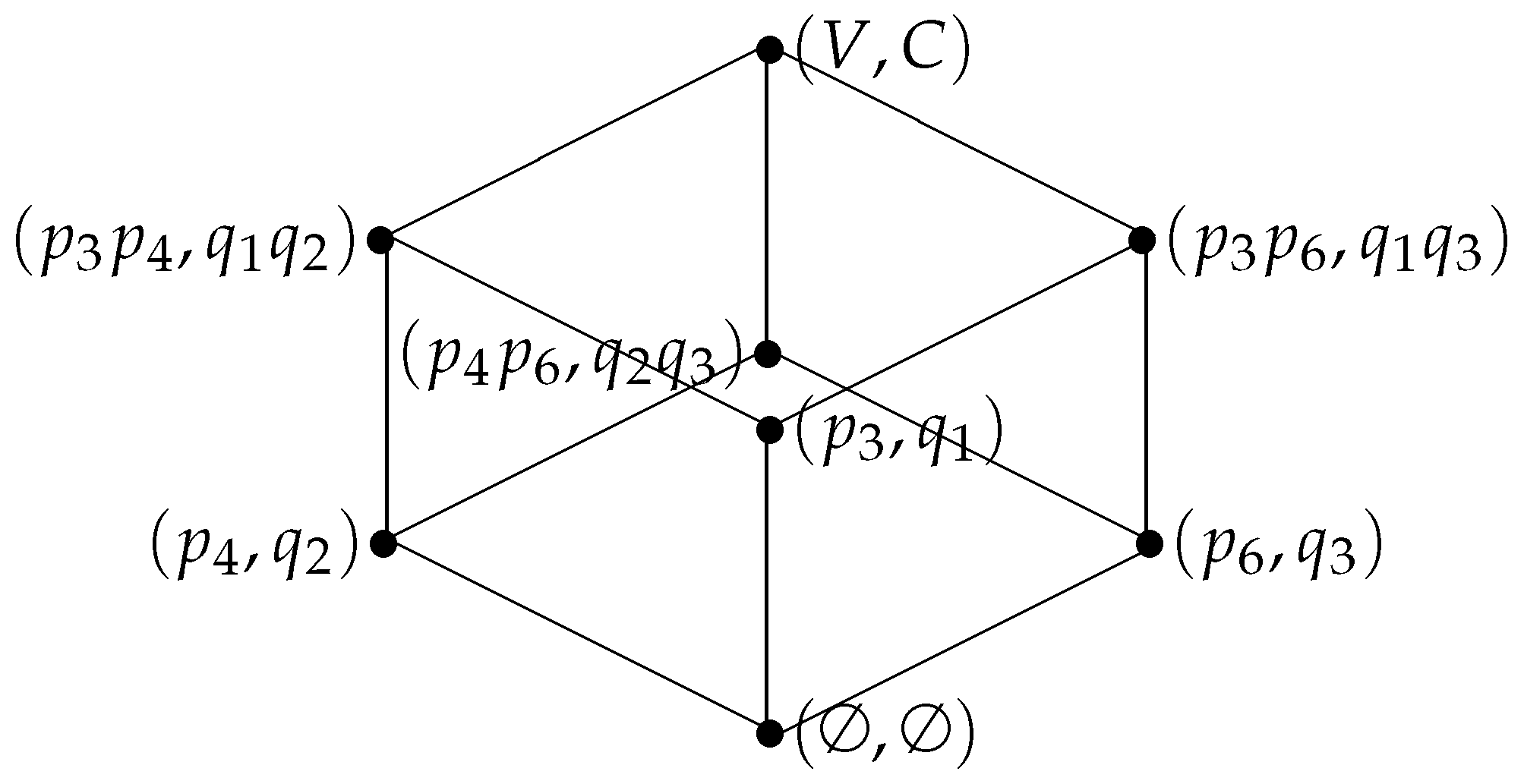
Let $V=\{p_3,p_4,p_6\}$ and $C=\{q_1,q_2,q_3\}$, then $(V,C,I_{V\times C})$ is a subcontext. Moreover, $\mathbb{O}(V,C,I_{V\times C})$= $\{(\varnothing ,\varnothing ),(p_3,q_1),(p_4,q_2),(p_6,q_3),(p_3{p}_4,q_1{q}_2),(p_3{p}_6,q_1{q}_3),(p_4{p}_6,q_2{q}_3),(V,C)\}\}.$ Figure 2 shows the Hasse diagram of $\mathbb{O}(V,C,I_{V\times C})$. Clearly, $\mathbb{O}(O,A,I)\cong \mathbb{O}(V,C,I_{V\times C})$.

The bireduction process is as follows.

$$\begin{array}{c}\left(\begin{array}{cccccc}& q_{1,4}& q_2& q_3& q_5& q_{6,7}\\ p_1& 1& & 1& 1& 1\\ p_2& & 1& 1& 1& 1\\ p_3& 1& & & 1& 1\\ p_{4,5}& & 1& & 1& \\ p_6& & & 1& & 1\end{array}\right)\overrightarrow{\frac{R_1-R_5}{R_2-R_5}}\left(\begin{array}{cccccc}& q_{1,4}& q_2& q_3& q_5& q_{6,7}\\ p_1& 1& & 0& 1& 0\\ p_2& & 1& 0& 1& 0\\ p_3& 1& & & 1& 1\\ p_{4,5}& & 1& & 1& \\ p_6& & & 1& & 1\end{array}\right)\overrightarrow{R_2-R_4}\\ \left(\begin{array}{cccccc}& q_{1,4}& q_2& q_3& q_5& q_{6,7}\\ p_1& 1& & 0& 1& 0\\ p_2& & 0& 0& 0& 0\\ p_3& 1& & & 1& 1\\ p_{4,5}& & 1& & 1& \\ p_6& & & 1& & 1\end{array}\right)\overrightarrow{R_1-R_3}\left(\begin{array}{cccccc}& q_{1,4}& q_2& q_3& q_5& q_{6,7}\\ p_1& 0& & 0& 0& -1\\ p_2& & 0& 0& 0& 0\\ p_3& 1& & & 1& 1\\ p_{4,5}& & 1& & 1& \\ p_6& & & 1& & 1\end{array}\right),\end{array}$$

where $p_{4,5}=\{p_4,p_5\}$. We obtain all object reducts $\{p_3,p_4,p_6\}$ and $\{p_3,p_5,p_6\}$.

We continue the reduction process with the following column operations.

$$\begin{array}{c}\left(\begin{array}{cccccc}& q_{1,4}& q_2& q_3& q_5& q_{6,7}\\ p_3& 1& & & 1& 1\\ p_{4,5}& & 1& & 1& \\ p_6& & & 1& & 1\end{array}\right)\overrightarrow{\frac{C_4-C_1}{C_5-C_1}}\left(\begin{array}{cccccc}& q_{1,4}& q_2& q_3& q_5& q_{6,7}\\ p_3& 1& & & 0& 0\\ p_{4,5}& & 1& & 1& \\ p_6& & & 1& & 1\end{array}\right)\overrightarrow{C_4-C_2}\\ \left(\begin{array}{cccccc}& q_{1,4}& q_2& q_3& q_5& q_{6,7}\\ p_3& 1& & & 0& 0\\ p_{4,5}& & 1& & 0& \\ p_6& & & 1& & 1\end{array}\right)\overrightarrow{C_5-C_3}\left(\begin{array}{cccccc}& q_{1,4}& q_2& q_3& q_5& q_{6,7}\\ p_3& 1& & & 0& 0\\ p_{4,5}& & 1& & 0& \\ p_6& & & 1& & 0\end{array}\right).\end{array}$$

We obtain all attribute reducts $\{q_1,q_2,q_3\}$ and $\{q_2,q_3,q_4\}$. Hence, we can derive all bireducts of S. As we can see from this example, identifying all bireducts of a context is just matrix transformation processes.

For a given context S, Theorem 1 tells us that $(Y,C)\in \mathbb{A}(O,A,I)\iff (C,Y)\in \mathbb{O}(A,O,I^{-1})$. Thus, attribute reduction, object reduction and bireduction for $\mathbb{A}(O,A,I)$ can be turned into object reduction, attribute reduction and bireduction for $\mathbb{O}(A,O,I^{-1})$, respectively.

(1) Attribute reduction for $\mathbb{A}(O,A,I)$ coincides with object reduction for $\mathbb{O}(A,O,I^{-1})$.

(2) Object reduction for $\mathbb{A}(O,A,I)$ coincides with attribute reduction for $\mathbb{O}(A,O,I^{-1})$.

(3) $(X,B)$ is a bireduct of $\mathbb{A}(O,A,I)$ if and only if $(B,X)$ is a bireduct of $\mathbb{O}(A,O,I^{-1})$.

Therefore, our proposed bireduction algorithm for OOCLs can be used to identify bireducts for AOCLs.

6. Conclusions

AOCL was proposed by Gediga and Duntsch, and OOCL was defined by Yao. The two types of concept lattices are an important bridge between FCA and RST. This paper has shown that the two types of lattices can be converted into each other. The reduction problem is an important topic in FCA, Liu et al. [30] considered the reduction problem in OOCLs and AOCLs and gave the corresponding reduction algorithms. However, their reduction algorithms are based on discernibility matrices and algorithm complexity is high. Virtually all contexts of practical importance are too large to be explored by hand. Thus, the algorithmic reduction implementation of the methods for exploring them is of great importance. In order to obtain simple reduction algorithms, we consider attribute reduction, object reduction and bireduction for OOCLs, respectively. The corresponding reduction algorithms are obtained and our proposed algorithms are much simpler than that of paper [30]. Moreover, our algorithms do not require calculating the concept lattice and corresponding discernibility matrix. In the future, we will extend our method to other types of reduction and consider the real-world applications of the proposed algorithm.