
Hybrid Fuzzy C-Means Clustering Algorithm Oriented to Big Data Realms

 , ,
, ,  , and
, and
Abstract
:1. Introduction
2. Related Work
3. Materials and Methods
3.1. K-Means Algorithm
| Algorithm 1: Standard K-Means | |
| 1 | Initialization: |
| 2 | X: = {x1, …, xn}; |
| 3 | V: = {v1, …, vk}; |
| 4 | Classification: |
| 5 | For xi ϵ X and vk ϵ V{ |
| 6 | Calculate the Euclidean distance from each xi to the k centroids; |
| 7 | Assign the xi object to the nearest vk centroid;} |
| 8 | Calculate centroids: |
| 9 | Calculate the centroid vk; |
| 10 | Convergence: |
| 11 | If V: = {v1, …, vk} does not change in two consecutive iterations: |
| 12 | Stop the algorithm; |
| 13 | Otherwise: |
| 14 | Go to Classification |
| 15 | End of algorithm |
3.2. K++ Algorithm
| Algorithm 2: K++ | |
| 1 | Initialization: |
| 2 | X: = {x1, …, xn}; |
| 3 | Assign the value for k; |
| 4 | V: = Ø; |
| 5 | Select the first randomly uniform k1 centroid V: = V U {v1} ; |
| 6 | For i = 2 to k: |
| 7 | Select the i-th centroid vi of X with probability D(xi, vj)/∑xϵX D(xi, vj); |
| 8 | V: = V U {vi} ; |
| 9 | End of for |
| 10 | Return V |
| 11 | End of algorithm |
3.3. O-K-Means Algorithm
| Algorithm 3: O-K-Means | |
| 1 | Initialization: |
| 2 | X: = {x1, …, xn}; |
| 3 | V: = {v1, …, vk}; |
| 4 | εok: = Threshold value for determining O-K-Means convergence; |
| 5 | Classification: |
| 6 | For xi ϵ X and vk ϵ V{ |
| 7 | Calculate the Euclidean distance from each xi to the k centroids; |
| 8 | Assign the xi object to the nearest vk centroid; |
| 9 | Compute γ}; |
| 10 | Calculate centroids: |
| 11 | Calculate the centroid vk; |
| 12 | Convergence: |
| 13 | If (γ ≤ εok): |
| 14 | Stop the algorithm; |
| 15 | Otherwise: |
| 16 | Go to Classification |
| 17 | End of algorithm |
3.4. FCM Algorithm
| Algorithm 4: Standard FCM | |
| 1 | Initialization: |
| 2 | Assign the value for c y m; |
| 3 | Determine the value of the threshold ε for convergence; |
| 4 | t: = 0, TMAX: = 50; |
| 5 | X: = {x1, …, xn}; |
| 6 | U(t): = {µ11, …, µij}; is randomly generated |
| 7 | Calculate centroids: |
| 8 | Calculate the centroid vk; |
| 9 | Classification: |
| 10 | Calculate and update the membership matrix U(t+1): = {µij} |
| 11 | Convergence: |
| 12 | If max [abs(µij(t) − µij(t+1))] < ε or t ≤ TMAX: |
| 13 | Stop the algorithm; |
| 14 | Otherwise: |
| 15 | U(t): = U(t+1) y t: = t + 1; |
| 16 | Go to Classification |
| 17 | End of algorithm |
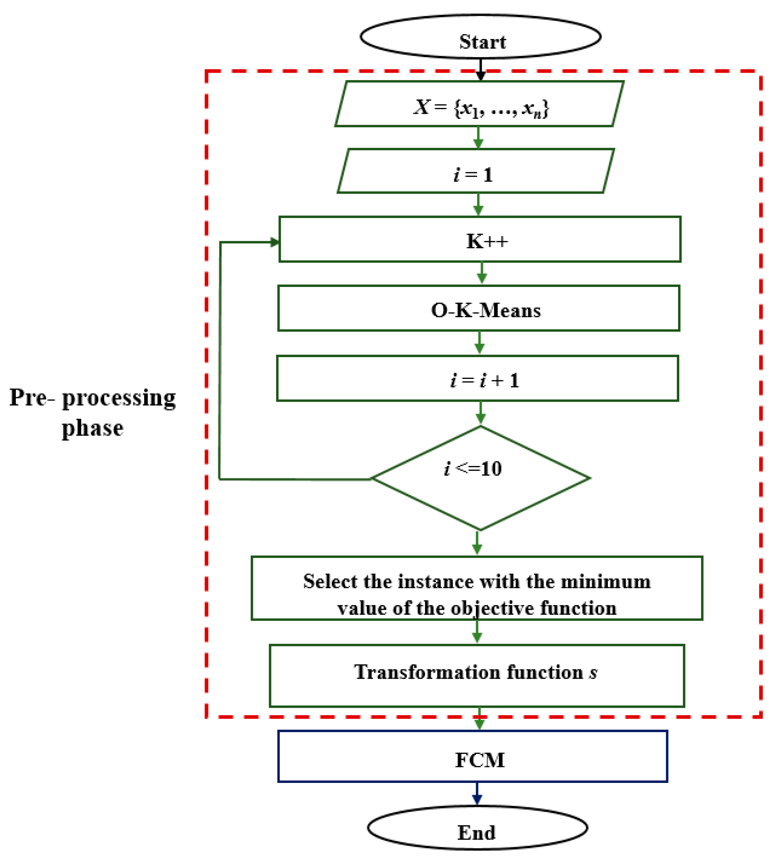
4. Proposal for Improvement
4.1. Transformation Functions
| Algorithm 5: HOFCM | |
| 1 | Initialization: |
| 2 | X: = {x1, …, xn}; |
| 3 | V: = {v1, …, vc}; |
| 4 | εok: = Threshold value for determining O-K-Means convergence; |
| 5 | Assign the value for c; |
| 6 | i: = 1; |
| 7 | Repeat |
| 8 | Function K++ (X, c): |
| 9 | Return V’; |
| 10 | Function O-K-Means (X, V″, εok, c): |
| 11 | Return V’’; |
| 12 | i = i + 1; |
| 13 | While i <=10; |
| 14 | Select V’’ for the value of i at which the objective function obtained the minimum value; |
| 15 | Transformation function s; |
| 16 | Determine the value of the threshold ε to determine the convergence of the algorithm; |
| 17 | Assign the value for m; |
| 18 | t: = 1; |
| 19 | Calculate centroids: |
| 20 | Calculate the centroid vj; |
| 21 | Classification: |
| 22 | Calculate and update the membership matrix U(t+1): = {µij}; |
| 23 | Convergence: |
| 24 | If max [abs(µij(t) − µij(t+1))] < ε: |
| 25 | Stop the algorithm; |
| 26 | Otherwise: |
| 27 | U(t): = U(t+1) y t: = t + 1; |
| 28 | Go to Classification |
| 29 | End of algorithm |
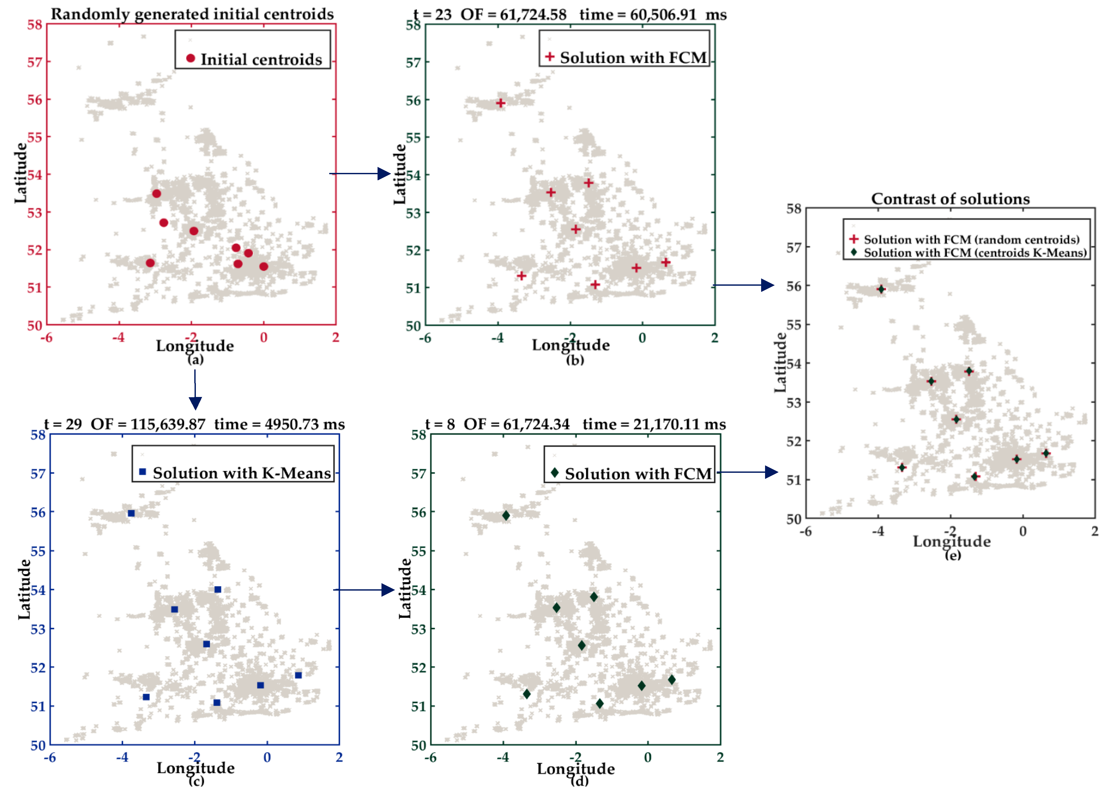
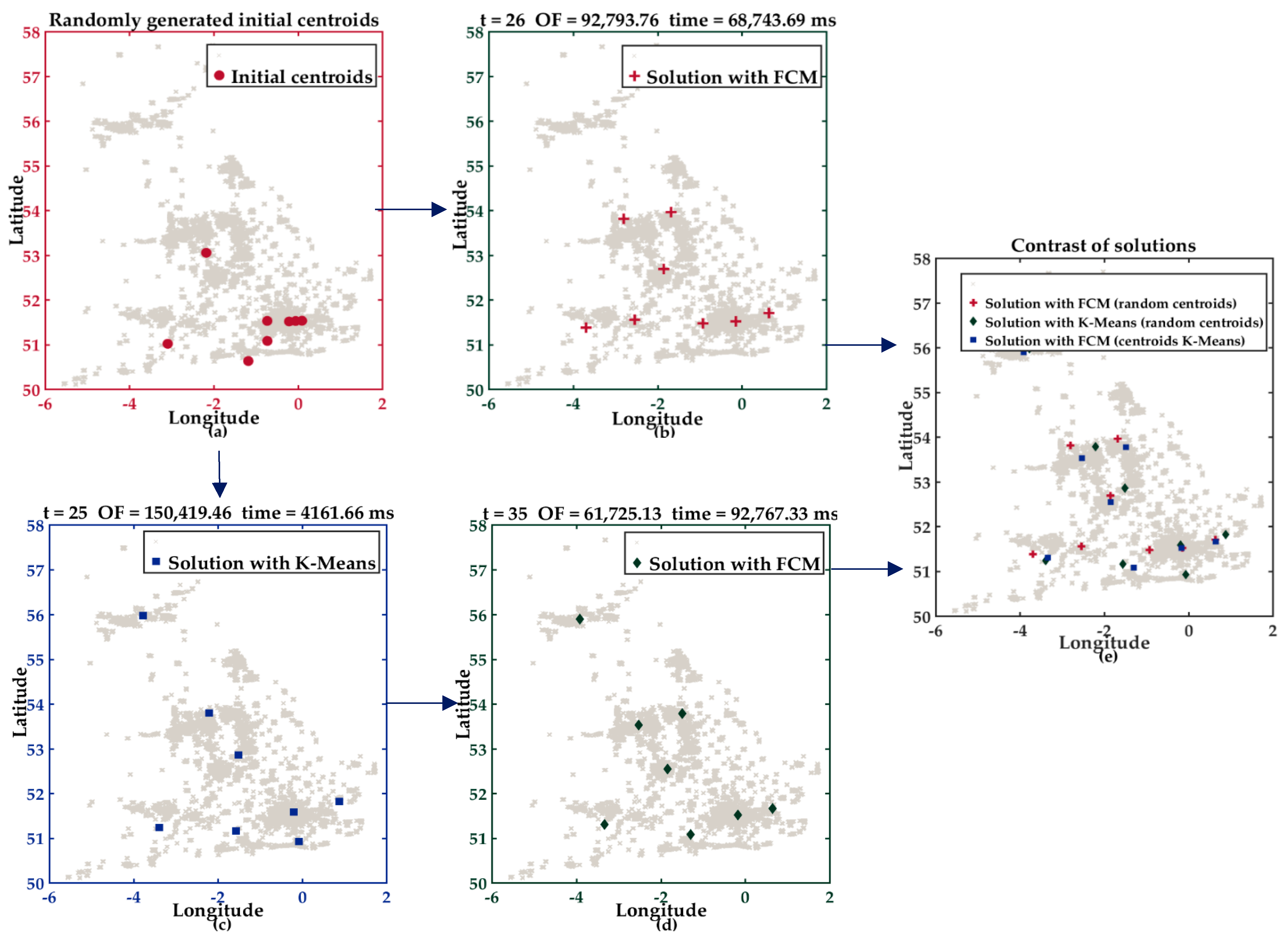
5. Results
5.1. Experiment Environment
5.2. Description of Test Cases
5.2.1. Description of Experiment I
5.2.2. Description of Experiment II
5.3. Analysis of Experiments
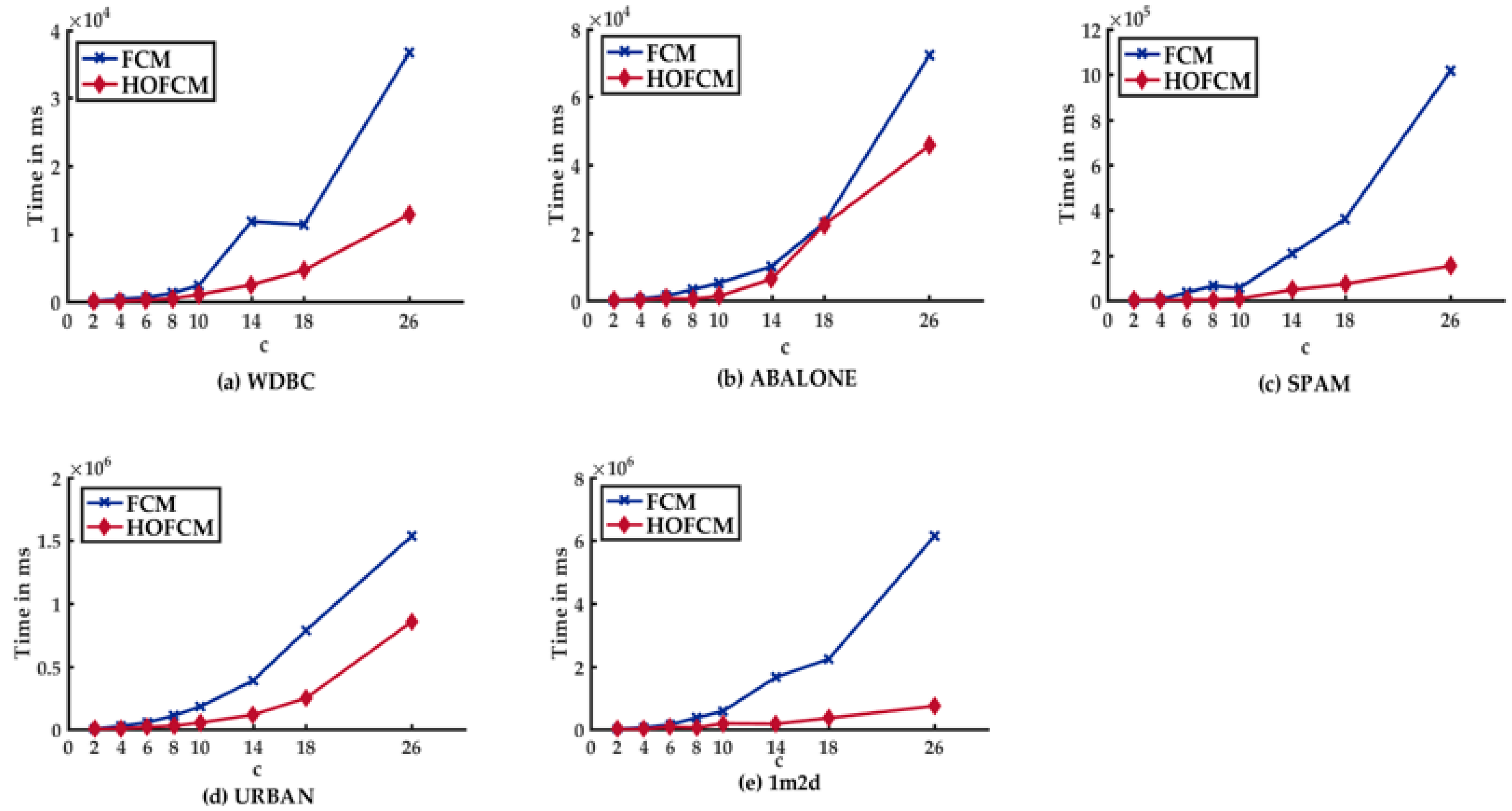
5.3.1. Analysis of the Results of Experiment I
- In the case of HOFCM, for all datasets, time was reduced in all test cases. In the best case, it was reduced by up to 93.94%. This percentage is highlighted in bold in column seven. Notably, this percentage was achieved with the SPAM dataset, which has high dimensionality.
- HOFCM improved the quality of the solution in large datasets in 20 of 24 cases. In the best case, the quality of the solution was enhanced by 68.31%. This percentage is highlighted in bold in column eight. In the worst case, a quality loss of 2.19% was identified, as can be seen in column four. Regarding the small datasets, a solution quality of 62.5% was obtained in all cases, that is, in 10 of the 16 test cases.
- In general, based on the results obtained, it is possible to affirm that the HOFCM proposal performs better than the standard FCM algorithm.
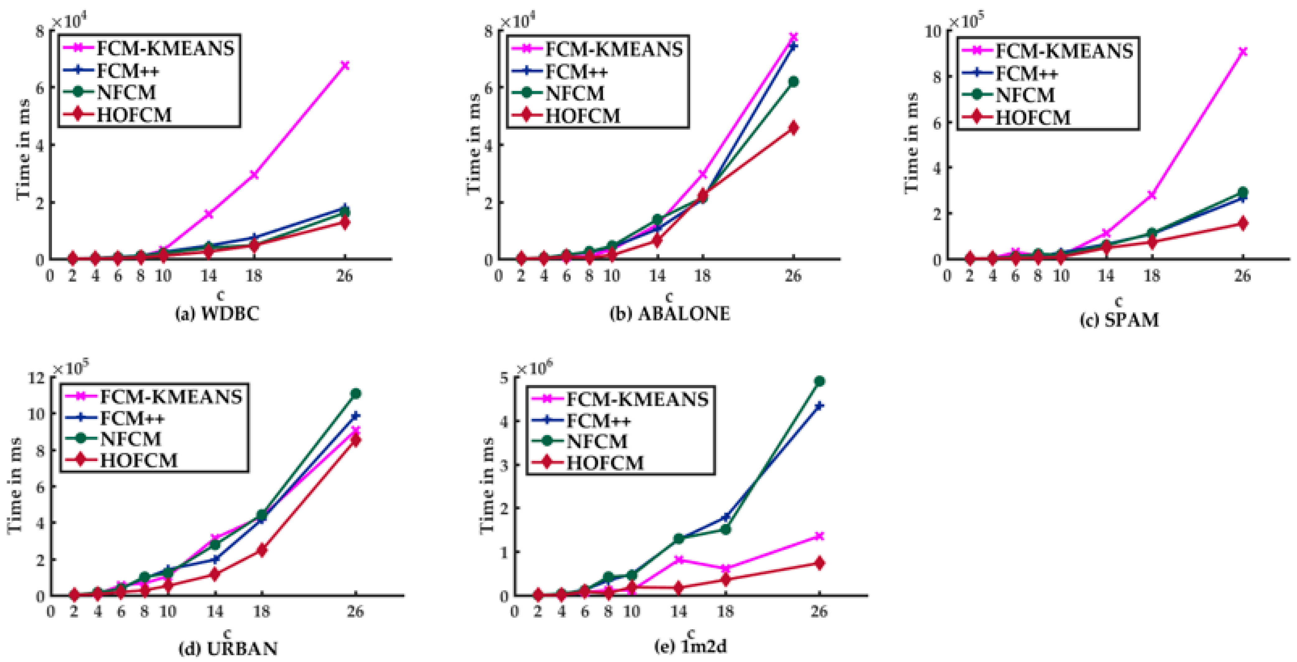
5.3.2. Analysis of the Results of Experiment II
- HOFCM outperformed the FCM++ algorithm in terms of solution time in all test cases with large datasets. In the small datasets, only in one case was it not higher. Regarding the quality of the solution in large datasets, in the best case, an average gain of 5.48% was obtained, and in the worst case, there was a loss of 2.33%. Both percentages are in bold in column eight in Table 3. It can be stated that HOFCM was higher in terms of solution quality in 75% of all cases.
- HOFCM outperformed the FCM-KMeans algorithm in solution quality in 82.5% of all test cases. Regarding the solution time, HOFCM was better in the large and real datasets.
- HOFCM outperformed the NFCM algorithm in solution quality in 85% of all test cases. Regarding the solution time, HOFCM was better in the large datasets.
- In all three comparisons, HOFCM obtained the greatest time reductions and the greatest gains in solution quality when dealing with large and real datasets.
- In general, based on the results obtained, it is possible to affirm that the HOFCM proposal performs better than the FCM++, FCM-KMeans, and NFCM algorithms.
6. Discussion
7. Conclusions
Author Contributions
Funding
Institutional Review Board Statement
Informed Consent Statement
Data Availability Statement
Conflicts of Interest
References
- Yang, M.S. A survey of fuzzy clustering. Math. Comput. Model. 1993, 18, 1–16. [Google Scholar] [CrossRef]
- Nayak, J.; Naik, B.; Behera, H.S. Fuzzy C-Means (FCM) Clustering Algorithm: A Decade Review from 2000 to 2014. In Proceedings of the Comput Intell Data Mining, Odisha, India, 20–21 December 2014. [Google Scholar]
- Shirkhorshidi, A.S.; Aghabozorgi, S.; Wah, T.Y.; Herawan, T. Big Data Clustering: A Review. In Proceedings of the International Conference on Computational Science and Its Applications—ICCSA 2014, Guimaraes, Portugal, 30 June–3 July 2014. [Google Scholar]
- Ajin, V.W.; Kumar, L.D. Big data and clustering algorithms. In Proceedings of the 2016 International Conference on Research Advances in Integrated Navigation Systems (RAINS), Bangalore, India, 6–7 April 2016. [Google Scholar]
- MacQueen, J. Some methods for classification and analysis of multivariate observations. In Proceedings of the 5th Berkeley Symp Math Statis and Probability, Berkeley, CA, USA, 21 June–18 July 1965. [Google Scholar]
- Ruspini, E.H.; Bezdek, J.C.; Keller, J.M. Fuzzy Clustering: A Historical Perspective. IEEE Comput. Intell. Mag. 2019, 14, 45–55. [Google Scholar] [CrossRef]
- Lee, G.M.; Gao, X. A Hybrid Approach Combining Fuzzy c-Means-Based Genetic Algorithm and Machine Learning for Predicting Job Cycle Times for Semiconductor Manufacturing. Appl. Sci. 2021, 11, 7428. [Google Scholar] [CrossRef]
- Lee, S.J.; Song, D.H.; Kim, K.B.; Park, H.J. Efficient Fuzzy Image Stretching for Automatic Ganglion Cyst Extraction Using Fuzzy C-Means Quantization. Appl. Sci. 2021, 11, 12094. [Google Scholar] [CrossRef]
- Ghosh, S.; Kumar, S. Comparative Analysis of K-Means and Fuzzy C-Means Algorithms. Int. J. Adv. Comput. Sci. Appl. 2013, 4, 35–39. [Google Scholar] [CrossRef] [Green Version]
- Garey, M.R.; Johnson, D.S. Computers and Intractability: A Guide to the Theory of NP-Completeness; W. H. Freeman & Co.: New York, NY, USA, 1979; pp. 109–120. [Google Scholar]
- Bezdek, J.C. Pattern Recognition with Fuzzy Objective Function Algorithms; Plenum Press: New York, NY, USA, 1981; pp. 43–93. [Google Scholar]
- Stetco, A.; Zeng, X.J.; Keane, J. Fuzzy C-means++: Fuzzy C-means with effective seeding initialization. Expert Syst. Appl. 2015, 42, 7541–7548. [Google Scholar] [CrossRef]
- Wu, Z.; Chen, G.; Yao, J. The Stock Classification Based on Entropy Weight Method and Improved Fuzzy C-means Algorithm. In Proceedings of the 2019 4th International Conference on Big Data and Computing, Guangzhou, China, 10–12 May 2019. [Google Scholar]
- Liu, Q.; Liu, J.; Li, M.; Zhou, Y. Approximation algorithms for fuzzy C-means problem based on seeding method. Theor. Comput. Sci. 2021, 885, 146–158. [Google Scholar] [CrossRef]
- Arthur, D.; Vassilvitskii, S. k-means++: The Advantages of Careful Seeding. In Proceedings of the Eighteenth Annual ACM-SIAM Symposium on Discrete Algorithms, New Orleans, LA, USA, 7–9 January 2007. [Google Scholar]
- Cai, W.; Chen, S.; Zhang, D. Fast and robust fuzzy c-means clustering algorithms incorporating local information for image segmentation. Pattern Recognit. 2007, 40, 825–838. [Google Scholar] [CrossRef] [Green Version]
- Al-Ayyoub, M.; Al-andoli, M.; Jararweh, Y.; Smadi, M.; Gupta, B.B. Improving fuzzy C-mean-based community detection in social networks using dynamic parallelism. Comput Elect. Eng. 2018, 74, 533–546. [Google Scholar] [CrossRef]
- Hashemzadeh, M.; Oskouei, A.G.; Farajzadeh, N. New fuzzy C-means clustering method based on feature-weight and cluster-weight learning. Appl. Soft. Comput. 2019, 78, 324–345. [Google Scholar] [CrossRef]
- Khang, T.D.; Vuong, N.D.; Tran, M.-K.; Fowler, M. Fuzzy C-Means Clustering Algorithm with Multiple Fuzzification Coefficients. Algorithms 2020, 13, 158. [Google Scholar] [CrossRef]
- Khang, T.D.; Tran, M.-K.; Fowler, M. A Novel Semi-Supervised Fuzzy C-Means Clustering Algorithm Using Multiple Fuzzification Coefficients. Algorithms 2021, 14, 258. [Google Scholar] [CrossRef]
- Naldi, M.C.; Campello, R.J.G.B. Comparison of distributed evolutionary k-means clustering algorithms. Neurocomputing 2015, 163, 78–93. [Google Scholar] [CrossRef]
- Pérez, J.; Almanza, N.N.; Romero, D. Balancing effort and benefit of K-means clustering algorithms in Big Data realms. PLoS ONE. 2018, 13, e0201874. [Google Scholar]
- Selim, S.Z.; Ismail, M.A. K-Means-Type Algorithms: A Generalized Convergence Theorem and Characterization of Local Optimality. IEEE Trans. Pattern Anal. Mach. Intell. 1984, PAMI-6, 81–87. [Google Scholar] [CrossRef]
- Jancey, R.C. Multidimensional group analysis. Aust. J. Bot. 1966, 14, 127–130. [Google Scholar] [CrossRef]
- Zadeh, L.A. Fuzzy sets. Inf. Control 1965, 8, 338–353. [Google Scholar] [CrossRef] [Green Version]
- Bellman, R.; Kalaba, R.; Zadeh, L.A. Abstraction and pattern classification. J. Math. Anal. Appl. 1966, 13, 1–7. [Google Scholar] [CrossRef]
- Ruspini, E.H. A new approach to clustering. Inf. Control 1969, 15, 22–32. [Google Scholar] [CrossRef] [Green Version]
- Dunn, J.C. A Fuzzy Relative of the ISODATA Process and Its Use in Detecting Compact Well-Separated Clusters. J. Cybern. 1974, 3, 32–57. [Google Scholar] [CrossRef]
- UCI Machine Learning Repository, University of California. Available online: https://archive.ics.uci.edu/ml/index.php (accessed on 26 January 2022).
- Rosen, K.H. Discrete Mathematics and Its Applications; McGraw-Hill Education: New York, NY, USA, 2018; pp. 90–98. [Google Scholar]
- McGeoch, C.C. A Guide to Experimental Algorithmics; Cambridge University Press: Cambridge, UK, 2012; pp. 17–114. [Google Scholar]


| Id | Name | Type | n | d | Size Indicator n*d |
|---|---|---|---|---|---|
| 1 | WDBC | Real | 569 | 30 | 17,070 |
| 2 | ABALONE | Real | 4177 | 7 | 29,239 |
| 3 | SPAM | Real | 4601 | 57 | 262,257 |
| 4 | URBAN | Real | 360,177 | 2 | 720,354 |
| 5 | 1m2d | Synthetic | 1,000,000 | 2 | 2,000,000 |
| Standard FCM versus HOFCM | |||||||||||
|---|---|---|---|---|---|---|---|---|---|---|---|
| WDBC | ABALONE | SPAM | URBAN | ||||||||
| P | c | % time | % Jm | % time | % Jm | % time | % Jm | % time | % Jm | % time | % Jm |
| 1 | 2 | 80.88 | 0.00 | 64.14 | 0.0035 | 54.37 | −0.001 | 46.12 | 4.12 | 74.95 | 0.03 |
| 2 | 4 | 87.12 | 0.02 | 56.15 | −0.02 | 75.36 | 6.53 | 76.33 | −0.001 | 87.81 | 0.03 |
| 3 | 6 | 67.83 | −2.19 | 52.59 | 0.00 | 92.58 | 22.75 | 68.18 | 0.07 | 45.26 | 0.36 |
| 4 | 8 | 64.30 | −1.17 | 86.60 | 0.08 | 93.94 | 36.90 | 74.60 | 1.42 | 85.56 | 0.22 |
| 5 | 10 | 57.55 | 3.03 | 75.61 | 0.09 | 86.22 | 50.69 | 70.98 | 1.85 | 67.75 | −0.05 |
| 6 | 14 | 78.99 | 4.50 | 37.00 | −0.11 | 77.20 | 49.30 | 70.38 | 4.26 | 89.65 | −0.27 |
| 7 | 18 | 59.04 | 12.39 | 2.71 | −0.60 | 79.80 | 56.24 | 68.45 | 7.81 | 84.07 | 0.05 |
| 8 | 26 | 64.99 | 27.31 | 36.78 | −2.05 | 84.88 | 68.31 | 44.38 | 10.73 | 88.00 | 0.02 |
| HOFCM versus FCM++ | |||||||||||
|---|---|---|---|---|---|---|---|---|---|---|---|
| WDBC | ABALONE | SPAM | URBAN | 1m2d | |||||||
| P | c | % time | % Jm | % time | % Jm | % time | % Jm | % time | % Jm | % time | % Jm |
| 1 | 2 | 66.87 | 0.00 | 59.38 | 0.00 | 41.67 | 0.00 | 18.19 | 0.00 | 32.08 | 0.03 |
| 2 | 4 | 78.59 | 0.02 | 36.47 | −0.02 | 53.08 | 0.01 | 52.36 | 0.00 | 73.61 | 0.03 |
| 3 | 6 | 69.42 | −0.52 | 54.03 | 0.04 | 54.04 | 5.48 | 54.83 | 1.86 | 37.78 | −0.01 |
| 4 | 8 | 57.86 | −0.20 | 80.64 | 0.05 | 60.42 | 1.97 | 70.42 | 2.20 | 84.36 | 0.02 |
| 5 | 10 | 57.29 | 1.76 | 68.80 | 0.09 | 71.62 | −2.33 | 63.27 | 1.70 | 62.20 | −0.07 |
| 6 | 14 | 45.97 | 0.43 | 39.00 | 0.04 | 25.56 | 2.77 | 41.40 | 2.10 | 86.60 | −0.19 |
| 7 | 18 | 37.01 | 0.18 | −7.22 | −0.06 | 32.72 | 0.94 | 40.44 | 3.57 | 80.08 | −0.03 |
| 8 | 26 | 27.58 | 2.92 | 38.48 | −0.71 | 42.08 | 2.24 | 13.33 | 0.62 | 82.99 | 0.09 |
| HOFCM versus FCM-KMeans | |||||||||||
|---|---|---|---|---|---|---|---|---|---|---|---|
| WDBC | ABALONE | SPAM | URBAN | 1m2d | |||||||
| P | c | % time | % Jm | % time | % Jm | % time | % Jm | % time | % Jm | % time | % Jm |
| 1 | 2 | 20.05 | 0.00 | 15.52 | 0.00 | 33.95 | 0.00 | 30.15 | 0.00 | 55.79 | 0.03 |
| 2 | 4 | 23.74 | 0.00 | 9.72 | 0.01 | 58.11 | 6.53 | 28.55 | 0.00 | 47.73 | 0.00 |
| 3 | 6 | 32.29 | −2.51 | −10.98 | 0.00 | 90.88 | 22.75 | 68.57 | 0.97 | −13.94 | 0.42 |
| 4 | 8 | 47.87 | −1.28 | 50.98 | −0.02 | 72.58 | 14.66 | 58.99 | 0.14 | 53.89 | −0.02 |
| 5 | 10 | 66.05 | 3.09 | 60.49 | 0.12 | 41.19 | 33.65 | 49.89 | 3.56 | −63.13 | 0.05 |
| 6 | 14 | 84.13 | 4.52 | 46.83 | 0.69 | 57.67 | 50.13 | 63.45 | 2.17 | 78.87 | 0.06 |
| 7 | 18 | 84.21 | 11.99 | 24.45 | −0.06 | 73.88 | 57.61 | 42.56 | 9.40 | 41.81 | 0.02 |
| 8 | 26 | 80.98 | 29.01 | 41.00 | −0.81 | 83.03 | 66.86 | 5.55 | 3.99 | 45.48 | −0.01 |
| HOFCM versus NFCM | |||||||||||
|---|---|---|---|---|---|---|---|---|---|---|---|
| WDBC | ABALONE | SPAM | URBAN | 1m2d | |||||||
| P | c | % time | % Jm | % time | % Jm | % time | % Jm | % time | % Jm | % time | % Jm |
| 1 | 2 | 74.65 | 0.01 | 61.84 | 0.00 | 47.58 | 0.00 | 18.43 | 0.00 | 19.79 | 0.03 |
| 2 | 4 | 76.70 | 3.74 | 44.02 | −0.02 | 55.53 | 4.66 | 60.83 | 0.00 | 82.07 | 0.03 |
| 3 | 6 | 61.78 | −1.09 | 51.07 | 0.02 | 75.69 | 4.77 | 54.85 | 2.34 | 30.90 | 0.13 |
| 4 | 8 | 55.55 | −0.30 | 82.67 | 0.76 | 81.25 | 9.07 | 72.68 | 1.81 | 87.45 | 0.01 |
| 5 | 10 | 48.54 | 3.21 | 71.65 | 0.46 | 55.00 | 20.87 | 56.78 | 3.77 | 59.43 | 0.16 |
| 6 | 14 | 35.87 | 1.15 | 53.76 | 0.17 | 19.88 | 12.98 | 58.73 | 2.38 | 86.76 | −0.15 |
| 7 | 18 | 1.49 | 2.63 | −4.36 | −0.40 | 34.42 | 1.35 | 44.02 | 3.29 | 76.42 | 0.12 |
| 8 | 26 | 20.09 | 4.98 | 26.10 | −2.02 | 47.18 | 5.33 | 22.79 | 3.47 | 84.93 | 0.14 |
| Algorithm Dataset Name | Standard FCM | FCM-KMeans | FCM++ | NFCM | HOFCM |
|---|---|---|---|---|---|
| WDBC | 64,516.85 | 116,784.57 | 34,037.94 | 28,395.16 | 21,689.84 |
| ABALONE | 115,702.20 | 123,930.39 | 113,680.29 | 105,730.07 | 76,996.63 |
| SPAM | 1,746,301.34 | 1,355,655.16 | 482,874.71 | 513,205.42 | 289,610.79 |
| URBAN | 3,080,009.70 | 1,886,664.03 | 1,885,697.60 | 2,104,360.89 | 1,321,799.74 |
| 1m2d | 11,181,675.94 | 3,091,877.12 | 8,385,299.13 | 8,729,514.14 | 1,592,132.11 |
| The total sum of solution time | 16,188,206.03 | 6,574,911.27 | 10,901,589.67 | 11,481,205.68 | 3,302,229.11 * |
| The number of times by which the HOFCM algorithm is faster | 4.90 | 1.99 | 3.30 | 3.48 |
Publisher’s Note: MDPI stays neutral with regard to jurisdictional claims in published maps and institutional affiliations. |
© 2022 by the authors. Licensee MDPI, Basel, Switzerland. This article is an open access article distributed under the terms and conditions of the Creative Commons Attribution (CC BY) license (https://creativecommons.org/licenses/by/4.0/).
Share and Cite
Pérez-Ortega, J.; Roblero-Aguilar, S.S.; Almanza-Ortega, N.N.; Frausto Solís, J.; Zavala-Díaz, C.; Hernández, Y.; Landero-Nájera, V. Hybrid Fuzzy C-Means Clustering Algorithm Oriented to Big Data Realms. Axioms 2022, 11, 377. https://doi.org/10.3390/axioms11080377
Pérez-Ortega J, Roblero-Aguilar SS, Almanza-Ortega NN, Frausto Solís J, Zavala-Díaz C, Hernández Y, Landero-Nájera V. Hybrid Fuzzy C-Means Clustering Algorithm Oriented to Big Data Realms. Axioms. 2022; 11(8):377. https://doi.org/10.3390/axioms11080377
Chicago/Turabian StylePérez-Ortega, Joaquín, Sandra Silvia Roblero-Aguilar, Nelva Nely Almanza-Ortega, Juan Frausto Solís, Crispín Zavala-Díaz, Yasmín Hernández, and Vanesa Landero-Nájera. 2022. "Hybrid Fuzzy C-Means Clustering Algorithm Oriented to Big Data Realms" Axioms 11, no. 8: 377. https://doi.org/10.3390/axioms11080377
APA StylePérez-Ortega, J., Roblero-Aguilar, S. S., Almanza-Ortega, N. N., Frausto Solís, J., Zavala-Díaz, C., Hernández, Y., & Landero-Nájera, V. (2022). Hybrid Fuzzy C-Means Clustering Algorithm Oriented to Big Data Realms. Axioms, 11(8), 377. https://doi.org/10.3390/axioms11080377