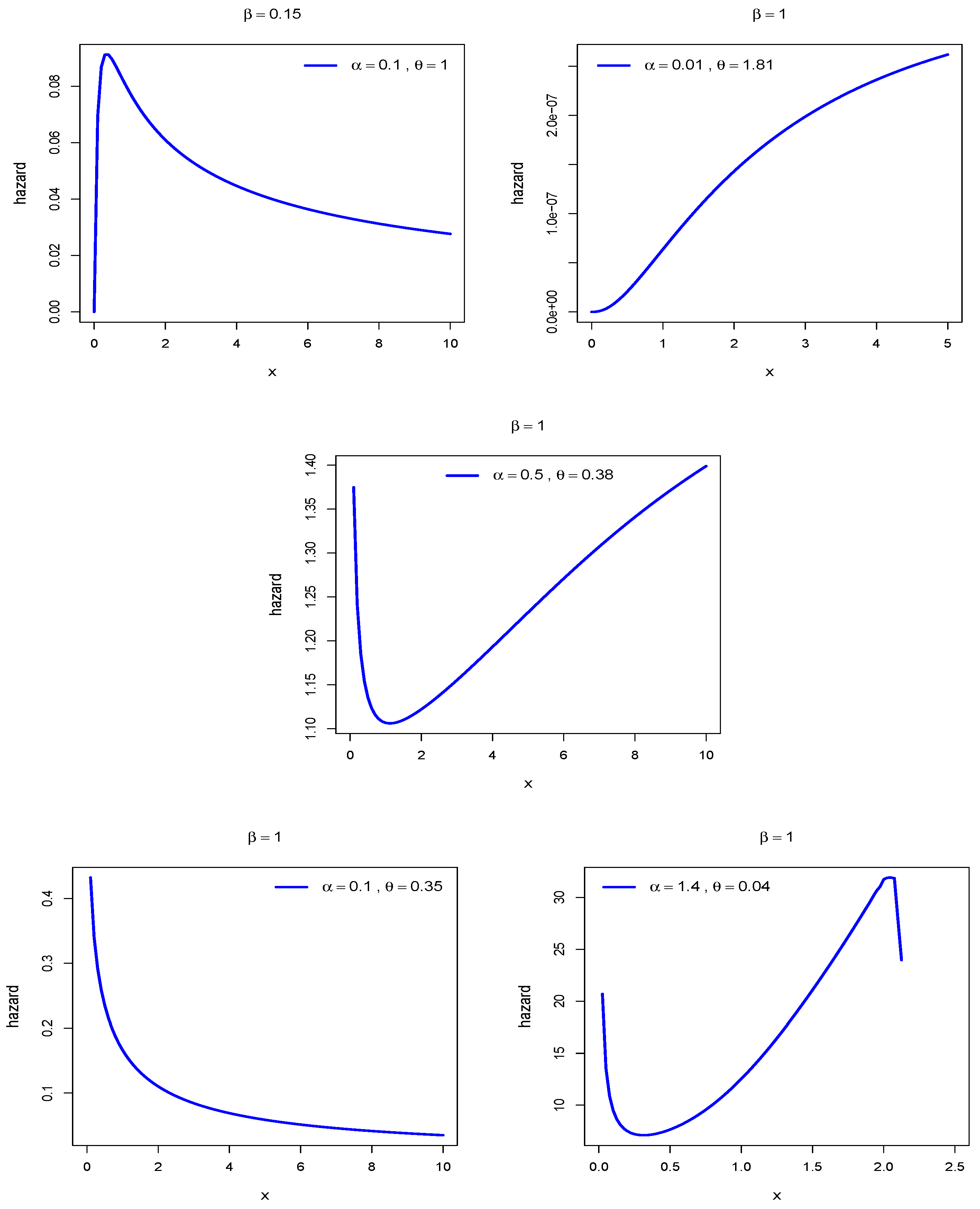
Article

A New Family of Lifetime Models: Theoretical Developments with Applications in Biomedical and Environmental Data

1
Department of Mathematics and Statistics, College of Science, Imam Mohammad Ibn Saud Islamic University (IMSIU), Riyadh 11432, Saudi Arabia
2
Faculty of Graduate Studies for Statistical Research, Cairo University, Giza 12613, Egypt
3
Department of Statistics, The Islamia University of Bahawalpur, Bahawalpur 63100, Pakistan
4
Department of Mathematics, Mirpur University of Science and Technology (MUST), Mirpur 10250, Pakistan
5
The Higher Institute of Commercial Sciences, Al Mahalla Al Kubra 31951, Egypt
6
Department of Statistics and Insurance, Faculty of Commerce, Zagazig University, Zagazig 44511, Egypt
7
Department of Basic, Sciences Higher Institute of Administrative Sciences, Osim, Cairo 12961, Egypt
*
Author to whom correspondence should be addressed.
Axioms 2022, 11(8), 361; https://doi.org/10.3390/axioms11080361
Submission received: 29 June 2022 / Revised: 14 July 2022 / Accepted: 18 July 2022 / Published: 25 July 2022
(This article belongs to the Special Issue Applied Mathematics in Biology and Medicine)

Abstract

:
With the aim of identifying a probability model that not only correctly describes the stochastic behavior of extreme environmental factors such as excess rain, acid rain pH level, and concentrations of ozone, but also measures concentrations of NO 2 and leads deliberations, etc., for a specific site or multiple site forms as well as for life testing experiments, we introduced a novel class of distributions known as the Sine Burr X G family. Some exceptional prototypes of this class are proposed. Statistical assets of the presented class, such as density function, complete and incomplete moments, average deviation, and Lorenz and Bonferroni graphs, are proposed. Parameter estimation is made via the likelihood method. Moreover, the application is explained by using four real data sets. We have also illustrated the significance and elasticity of the proposed class in the above-mentioned stochastic phenomenon.

1. Introduction

Several researchers have offered approaches for introducing probability models as examples. This phenomenon of adding parameters innovates more robust families of distributions, which are being effectively used for modeling engineering, economics, biological studies and environmental sciences data sets. Therefore, in this regard, some famous classes are the Marshall Olkin- G by [1], beta- G by [2], the Kumaraswamy- G studied by [3], odd Fréchet- G by [4] logistic- G by [5], exponentiated generalized- G proposed by [6], odd generalized N-H- G by [7], T - X class by [8], transmuted odd Fréchet- G by [9], exponentiated power generalized Weibull power series- G by [10], the Weibull- G by [11], the exponentiated half-logistic generated family by [12], Type II half logistic class by the odd [13], bivariate Weibull-G family by [14], exponentiated generalized alpha power family of distributions by [15], truncated Cauchy power Weibull-G class of distributions by [16], odd Perks-G class of distributions by [17], Type I half logistic Burr X-G family by [18], sine Topp-Leone-G family of distributions by [19], exponentiated version of the M family of distributions by [20], a new power Topp-Leone generated family of distributions by [21], truncated inverted Kumaraswamy generated family of distributions by [22], generalized exponential class discussed by [23], the beta odd log-logistic generalized studied by [24], alpha power transformation family of distributions introduced by [25], the Kumaraswamy exponential Pareto proposed by [26], the generalized Burr XII power series(GBXIIPS) class studied by [27], additive Weibull geometric (AWG) distribution proposed by [28] and the beta exponentiated modified Weibull (BEMW) distribution developed by [29], among others. However, in recent years, Ref. [30] presented another idea of generating to obtain a new life distribution by modification of trigonometric functions to give new statistical distributions. They transformed the sine function into a new statistical distribution called the sine- G class, with the cumulative distribution function (cdf) and probability density function (pdf) expressed as
F ( x ) = sin ( π 2 G ( x ) ) ,
and
f ( x ) = π 2 g ( x ) cos ( π 2 H ( x ) ) ,
respectively. The failure rate function (hrf) is defined as
ξ ( x ) = π 2 g ( x ) tan ( π 4 ( 1 + H ( x ) ) ) .
Some motivational factors of this family are: in its simple form, the two cumulative functions G ( x ) and H ( x ) possess an equal number of parameters, and it always avoids the problem of over parametrization, i.e., no additional parameters. In addition, cdf ( F ( x ) ) possesses the capability of surging the tractability of H ( x ) , offering new adaptable classes. Until recently, new trigonometric families of probability models developed thus far include β -trigonometric model studied by [31], sine square distribution discussed by [32], a cosine approximation to the normal distribution by [33], odd hyperbolic cosine exponential–exponential distribution by [34], odd hyperbolic cosine family of lifetime distributions by [35], transmuted arcsine distribution properties and application by [36], the arcsine exponentiated- X family by [37], among others. These are very complicated models that are seldom employed by applied practitioners. In order to create more feasible models using trigonometric functions, the challenge of avoiding non-identifiability issues is monumental. The proposed generalization is significant in this regard. Further, we must focus on developing a model that can capture all types of hazard rate curves. The sub-models of the ingenious family being studied in this article fulfills this aspect admirably. One key feature in proposing new generalizations include the continual improvement of the fits of new models when compared to conventional models using natural data sets. We are overwhelmed by the performance of the two sub-models fitted on four data sets, which outweighs twelve competitive well-established models, including four distributions with four parameters. Additionally, in order to quantify the similarity of the proposed model with its respective competing model using the same data, the Vuong test is used to compare the model fits that yielded significant findings, thus reinforcing the motivation in proposing the new family.
Ref. [38] introduced the Burr X G class of probability models. The cdf and pdf for the Burr X G family are expressed by
H BX ( x ; θ , δ ) = 1 e G ( x ; δ ) G ¯ ( x ; δ ) 2 θ ,
and
h BX ( x ; θ , δ ) = 2 θ g ( x ; δ ) G ( x ; δ ) 2 G ¯ ( x ; δ ) G ( x ; δ ) 3 e G ¯ ( x ; δ ) G ( x ; δ ) 2 1 e G ¯ ( x ; δ ) G ( x ; δ ) 2 θ 1 ,
respectively, and for comprehension, we can call G ¯ ( x ; δ ) = 1 G ( x ; δ ) the survival function (sf) and also g ( x ; δ ) as the pdf of a certain baseline model relying on a vector of unknown δ . Here, we are going to propose a class of sine-created models by taking into account the Burr X class as the baseline distribution in the sine family. This new family is referred to as the Sine Burr X G ( SBX G ) class of models.
The remainder of the article is sketched as follows. Starting from the second section, an innovative extended generator, called the Sine Burr X G family, is presented, and its sub-models are discussed. The third section deals with the SBX G model, which is not a nonlinear combination of exponentiated G ( e x p G ) probability models. Statistical properties of the SBX G family are provided in the fourth section. Inference about the population parameter based on a maximum likelihood estimation (MLE) is performed in the fifth section. The sixth section deals with the application of the proposed family. The final section states the conclusion.

2. Ingenious Proposed G X Class

Here, we construct a relatively new flexible model of distributions called the Sine Burr X G ( SBX G ) family of distributions by inserting (3) into (1), and we obtain the cdf, which is expressed as
F SBX G ( x ) = sin π 2 { 1 e G ( x ; δ ) G ¯ ( x ; δ ) 2 } θ , x R ,
where the respective pdf is
f S B X G ( x ) = π θ g ( x ; δ ) G ( x ; δ ) 2 G ¯ ( x ; δ ) G ( x ; δ ) 3 e G ¯ ( x ; δ ) G ( x ; δ ) 2 1 e G ¯ ( x ; δ ) G ( x ; δ ) 2 θ 1 × cos π 2 1 e G ( x ; δ ) G ¯ ( x ; δ ) 2 θ ,
whereas the sf and hazard rate function (hrf) are expressed as
F ¯ SBX G ( x ) = 1 sin π 2 1 e G ( x ; δ ) G ¯ ( x ; δ ) 2 θ
and
ξ S B X G ( x ) = π θ g ( x ; δ ) G ( x ; δ ) 2 G ( x ; δ ) G ¯ ( x ; δ ) 3 e G ( x ; δ ) G ¯ ( x ; δ ) 2 1 e G ¯ ( x ; δ ) G ( x ; δ ) 2 θ 1 × tan π 4 1 + 1 e G ¯ ( x ; δ ) G ( x ; δ ) 2 θ .

2.1. Sub-Models of SBX G Family

In Table 1, we study four possible sub-models of the SBX G class. The sub-models of this class possess the parental distributions, i.e., Lomax, log-logistic, exponential, and Rayleigh models, which are presented in Table 1. Therefore, we have the cdf and pdf of these parent models.
From this table, we pick model 1 and 2, study their pdf and hrf shapes and apply them to four real-life data sets in Section 6.3 for a thorough analysis.

2.1.1. A Sine Burr X Lomax (SBXL) Probability Model

The cdf and pdf of sine Burr X Lomax distribution are
F SBX G ( x ) = sin π 2 1 e ( 1 + x β ) α 1 2 θ ,
and
f SBX G ( x ) = π θ α ( x + β β ) α 1 β ( x + β β ) 3 α ( 1 ( x + β β ) α ) e ( x + β β ) α 1 2 1 e ( x + β β ) α 1 2 θ 1 cos ( π 2 1 e ( x + β β ) α 1 2 θ ) .

2.1.2. A Sine Burr X Loglogistic (SBXLL) Probability Model

After substituting the loglogistic distribution’s cdf and pdf into (1) and (2), we obtain
F SBX G ( x ) = sin 1 2 e θ x 2 β 1 e θ x 2 β α π ,
and
f SBX G ( x ) = π α β θ e x 2 β θ e x 2 β θ 1 e x 2 β θ α 1 x 2 β 1 cos 1 2 e x 2 β θ 1 e x 2 β θ α π .
Remark 1.
This family of distributions has the ability to model the positively skewed and symmetrical data (Figure 1 and Figure 2) with decreasing failure rate, increasing failure rate, bathtub shape, upside-down bathtub and decreasing-increasing-decreasing failure data (Figure 3 and Figure 4) structure in an appropriate fashion.

2.1.3. A Sine Burr-X Exponential (SBXE) Distribution

If G ( x ) = e μ x 1 e μ x and g ( x ) = μ e μ x , then the cdf and pdf of the SBXE model (for x > 0 ) are given below
F SBX G ( x ) = sin π 2 1 e e μ x 1 2 θ ,
and
f SBX G ( x ) = π θ μ e μ x ( e μ x 1 ) e e 2 μ x 1 e μ x 2 1 e e μ x 1 2 θ 1 cos ( π 2 1 e e μ x 1 2 θ ) .

2.1.4. A Sine Burr X Rayleigh (SBXR) Probability Model

The incorporation of the Rayleigh distribution’s cdf and pdf into Equations (1) and (2) is given below
F SBX G ( x ) = sin π 2 1 e e ρ 2 x 2 1 2 θ ,
and
f SBX G ( x ) = π ρ θ x e 2 ρ 2 x 2 e ρ 2 x 2 1 e ρ 2 x 2 e e ρ 2 x 2 1 2 1 e e ρ 2 x 2 1 2 θ 1 cos ( π 2 1 e e ρ 2 x 2 1 2 θ ) .

3. Expansion of the SBX G Density Function

Here, we derived the pdf expansion of the Sine Burr X G   SBX G class of distributions. By applying the Taylor series expansion, we obtain,
cos π 2 G ( x ) = i = 0 ( 1 ) i ( 2 i ) ! π 2 G ( x ) 2 i .
We have
cos π 2 1 e G ( x ; δ ) G ¯ ( x ; δ ) 2 θ = i = 0 ( 1 ) i ( 2 i ) ! π 2 2 i 1 e G ( x ; δ ) G ¯ ( x ; δ ) 2 2 i θ .
Inserting (10) in (6), the SBX G density function reduces to
f SBX G ( x ) = i = 0 ( 1 ) i ( 2 i ) ! π 2 2 i π θ g ( x ; δ ) G ( x ; δ ) 2 G ¯ ( x ; δ ) G ( x ; δ ) 3 e G ( x ; δ ) G ¯ ( x ; δ ) 2 1 e G ¯ ( x ; δ ) G ( x ; δ ) 2 θ ( 2 i + 1 ) 1 ,
if a > 0 and z < 1 , the generalized binomial series expansion holds
( 1 z ) a 1 = k = 0 ( 1 ) k a 1 k z k ,
and on applying (12) to the last term in (11), we obtain
f SBX G ( x ) = i , j = 0 ( 1 ) i + j ( 2 i ) ! θ ( 2 i + 1 ) 1 j π 2 2 i π θ g ( x ; δ ) 1 G ¯ ( x ; δ ) 2 G ¯ ( x ; δ ) G ( x ; δ ) 3 e ( j + 1 ) G ( x ; δ ) G ¯ ( x ; δ ) 2 .
On expanding e ( j + 1 ) G ( x ; δ ) G ¯ ( x ; δ ) 2 , we obtain
e ( j + 1 ) G ¯ ( x ; δ ) G ( x ; δ ) 2 = m = 0 ( 1 ) m ( j + 1 ) m m ! G ( x ; δ ) 2 m G ¯ ( x ; δ ) 2 m .
Inserting the above term in (13), the SBX G density function becomes
f SBX G ( x ) = i , j = 0 k = 0 π θ ( 1 ) k ( j + 1 ) k k ! ( 1 ) i + j ( 2 i ) ! θ ( 2 i + 1 ) 1 j π 2 2 i g ( x ; δ ) G ¯ ( x ; δ ) 3 k G ( x ; δ ) 2 k 1 ,
where
( 1 z ) b = k = 0 ( 1 ) k b k z k ,
inserting (15) into (14) the SBX G , which is an infinite linear combination of Expo . G probability models
f SBX G ( x ) = d , m = 0 π d , m ξ d + 2 ( m + 1 ) ( x ) ,
where
π m , d = π θ i , j = 0 ( 1 ) i + j + k ( j + 1 ) m m ! ( 2 i ) ! ( 2 m + d + 2 ) θ ( 2 i + 1 ) 1 j π 2 2 i 2 m 3 d ,
and ξ d + 2 ( m + 1 ) ( x ) = ( d + 2 m + 2 ) g ( x ) G d + 2 m + 2 ( x ) is the expo . G pdf with power parameter d + 2 ( m + 1 ) . Thus, the SBX G probability model can be viewed as a mixture of infinite components of exponentiated G densities with parameters ( d + 2 + 2 m ) . Thus, several mathematical features of the SBX G model come directly from those of the e x p G model. In addition, the cdf of the SBX G family can be expressed as a mixture of exp G cdfs where
F STL G ( x ) = m , d = 0 π m , d ξ ( 2 ( m + 1 ) + d ) ( x ) .
where Π ( 2 ( m + 1 ) + d ) ( x ) is the exp G cdf with power parameter ( 2 ( m + 1 ) + d ) .

4. Mathematical and Statistical Properties

Here we shall study quantiles, moment generating, moments, conditional moments, mean deviation, Bonferroni and Lorenz and order statistics of the SBX G class of distribution.

4.1. Percentile Function

Suppose X to be a continuous variate, then its cumulative distribution function is expressed as F X : R [ 0 , 1 ] . Now, from this definition, a percentile function P generally sends back a threshold measurement x underneath which a haphazard draws from the given cdf would fall p percent of the time. In this regard, the inverse of the SBX G percentile function, yields x = P ( p ) as follows
F 1 ( p ) = P G ( p ) = G 1 log 1 2 π arcsin ( p ) 1 θ 1 2 1 + log 1 2 π arcsin ( p ) 1 θ 1 2 .
where P G ( p ) denotes the percentile function of G ( x ) . As P ( p ) is characterized by the equation F ( P ( p ) ) = P ( F ( p ) ) = p , p ( 0 , 1 ) . The median is given by
M e d i a n = G 1 log 1 2 π arcsin ( 0.5 ) 1 θ 1 2 1 + log 1 2 π arcsin ( 0.5 ) 1 θ 1 2
The skewness measure is due to the Bowley skewness defined by
SK = P ( 3 4 ) + P ( 1 4 ) 2 P ( 1 2 ) P ( 3 4 ) P ( 1 4 )
On the other hand, the Moors kurtosis (Moors, (1988)) based on quantiles is given by
KU = P ( 7 8 ) P ( 5 8 ) + P ( 3 8 ) P ( 1 8 ) P ( 6 8 ) P ( 2 8 ) .
where P ( ·) represents the percentile function. The measures SK and KU possess the usual characteristics.

4.2. Moment Generating Functions Cum Moments

In mathematics and statistics, moments of a function are reasonable procedures associated with the shape of the function’s graph. If the function represents density or mass function, then the first moment represents the center of the mass or expected value, and the second moment is the rotational inertia or the variance. Similarly, the ratio of the third mean moment to the square of the second mean moment is the skewness, and the ratio fourth moment about the mean to the second moment about the mean is the kurtosis. Moreover, these moments not only determine the shape of a function but also help to characterize the probability functions.
Let Z ( 2 ( m + 1 ) + d ) ) be a stochastic variate possessing exp G pdf π ( d + 2 ( m + 1 ) ) ) with power parameter ( d + 2 ( m + 1 ) ) ) . The s t h moment of a SBX G class of distributions can be obtained from (16)
μ s / = E ( X s ) = d = 0 = m π d , m E ( Z ( d + 2 ( m + 1 ) ) ) s )
where Z ( 2 ( m + 1 ) + d ) denotes the exponentiated G distribution with power parameter d + 2 ( m + 1 ) . Another formula for the s t h moment follows from (16) as
μ s / = E ( X s ) = d , m = 0 π d , m E ( Z ( d + 2 ( m + 1 ) ) ) s )
where
E ( Z ϑ s ) = ϑ x r g ( x ) G ( x ) ϑ 1 , ν > 0
can be estimated in terms of the baseline percentile function, i.e., P G ( p ) = G 1 ( p ) as
E ( Z ϑ s ) = ϑ 0 1 p ϑ 1 P G ( p ) s d p .
Now we introduce two formulae for the moment generating function. The initial rule can be compiled from Equation (16) as given by
M X ( t ) = E ( e t X ) = d = 0 = m ϖ d , m M k + 1 ( t ) ,
where M ( 2 ( m + 1 ) + d ) ) ( t ) is the moment generating function of Z ( d + 2 ( m + 1 ) ) ) . Consequently, we can easily determine M X ( t ) from the exp G generating function. The second formula for the M X ( t ) follows from (16) as
M X ( t ) = E ( e t X ) = d , m = 0 ϖ d , m M ( 2 ( m + 1 ) + d ) ) ( t )
where M ϰ ( t ) is the mgf of random variable Z ϰ given by
M ϰ ( t ) = e t X g ( x ) G ( x ) ϰ 1 , ϰ > 0 = ϰ 0 1 u ϰ 1 e t P G ( u ) d u
which can be compiled numerically by using the baseline percentile function, i.e., P G ( p ) = G 1 ( p ) .  Table 2 and Table 3 give a numerical analysis for the mean M ( X ) , variance V a r ( x ) , skewness C S ( x ) , kurtosis C K ( x ) and coefficient of variation C V ( x ) for SBXL and SBXLL models, respectively.
Figure 5 and Figure 6 represent the 3-D plots of the M ( x ) , V a r ( x ) , C S ( x ) and C K ( x ) of the SBXL and SBXLL distributions, respectively, for several values of parameters.

4.3. Conditional Moments

Prediction via lifetime probability models compels researchers to adopt the conditional moments methodology, the average residual lifetime function and mean inactivity time function. In this section, we focussed ourselves on the initial partial moment, which points out the Lorenz cum Bonferroni graphs, which are helpful in demography, econometrics, medicine, survival analysis and indemnity applications. Therefore, for this, the r t h partial moments of the variate X defined as δ r ( t ) for any real r > 0 is given as
δ r ( t ) = t x r f ( x ) d x = d , m = 0 ϖ d , m t x r δ r , ( 2 ( m + 1 ) + d ) ) ( t ) d x
where
δ r , ν ( t ) = 0 G ( t ) u ν 1 P G ( p ) r d p
and δ r , ν ( t ) can be evaluated numerically.

4.3.1. Mean Deviation

The partial moments methodology is quite useful in finding the average deviance between the median and mean, where the median/mean aberration yields key evidence that is typical of a population. These partial moments can be used in many fields such as economics and insurance. Let stochastic measure X have the SBX G family of distribution. The mean deviations about the mean μ = E ( X ) and the mean deviations about the median M are defined by
δ 1 ( x ) = E X μ 1 / = 2 μ 1 / F ( μ 1 / ) 2 δ 1 ( μ 1 / )
and
δ 2 ( x ) = E X M = μ 1 / 2 δ 1 ( M )
respectively, where μ 1 / = E ( X ) , M = m e d i a n (X) = Q ( 1 2 ) , and δ 1 ( t ) is the first complete moment given by (20) with s = 1 .

4.3.2. Bonferroni and Lorenz Curves

For a positive stochastic variate X, the Lorenz and Bonferroni curves, for a given probability p , are given by L ( p ) = 1 μ 1 / δ 1 ( q ) and B ( p ) = 1 p μ 1 / δ 1 ( q ) , respectively, where μ 1 / = E ( X ) , and p = P ( p ) is the percentile function of X at percentile p.

4.4. Order Statistics

Order observations are precise and important statistical measurements that covenant with the order data. One can define them by letting X 1 , X 2 ,…, X n be independent stochastic variates following the SBX G family of distributions of size n and letting the arrangement of these variates in ascending order be X ( 1 ) , X ( 2 ) ,…, X ( n ) , then the variates X ( 1 ) X ( 2 ) …≤ X ( n ) are ordered statistics of random variables. These ordered observations are frequently used in the reliability analysis of a system. The cumulative distribution function of i t h order statistics is expressed as follows
F i ; n ( x ) = 1 B ( i , n i + 1 ) j = 0 n i ( 1 ) j i + j n i j F i + j ( x ) = 1 B ( i , n i + 1 ) j = 0 n i ( 1 ) j n i j sin π 2 1 e G ( x ; δ ) G ¯ ( x ; δ ) 2 θ i + j
The corresponding pdf is expressed in the given form as
f i ; n ( x ) = f ( x ) B ( i , n i + 1 ) j = 0 n i ( 1 ) j n i j F i + j 1 ( x ) = 1 B ( i , n i + 1 ) j = 0 n i ( 1 ) j n i j π θ g ( x ; δ ) G ( x ; δ ) 2 G ( x ; δ ) G ¯ ( x ; δ ) 3 e G ¯ ( x ; δ ) G ( x ; δ ) 2 1 e G ( x ; δ ) G ¯ ( x ; δ ) 2 θ 1 cos ( π 2 1 e G ¯ ( x ; δ ) G ( x ; δ ) 2 θ ) sin π 2 1 e G ( x ; δ ) G ¯ ( x ; δ ) 2 θ i + j 1
Then the r t h moment of the i t h order statistics is given by
μ r = E ( X i : r r ) = x r f i ; n ( x ) d x = = 1 B ( i , n i + 1 ) j = 0 n i ( 1 ) j n i j x r f ( x ) F i + j 1 ( x ) d x = 1 B ( i , n i + 1 ) j = 0 n i ( 1 ) j n i j μ r , i + j 1
where this integral can be evaluated numerically.

5. Parameter Estimation

Method of Maximum Likelihood

Statistical implications are usually passed through three dissimilar methods such as interval and point estimation, as well as hypothesis testing. Although numerous methodologies for parameter estimation exist in the literature, the likelihood method is the most versatile one, which enjoys anticipated chattels when fabricating the confidence regions and intervals, as well as in test statistics. The asymptotic theory of these estimates convey simple calculations that toil well in limited information contained in the samples. Statisticians frequently pursue estimating quantities such as the density of a test statistic that depends on the sample size so as to obtain better estimate distributions. The subsequent calculations for the MLEs in distribution theory can be definitely handled either logically or mathematically. In this section, we are trying to cope with parameter estimation via the MLE method from the whole sample. Let x 1 , , x n be a stochastic realization of size n from the SBX G distribution given by (5). Let U n ( ϕ ) = ( n θ , n δ ) T be a q × 1 vector of the parameters. The log-likelihood function is given by
n = n log ( π ) + n log ( θ ) + i = 1 n log g ( x i ; δ ) + i = 1 n log G ( x i ; δ )
3 i = 1 n log ( G ¯ ( x i ; δ ) ) i = 1 n t i 2 + i = 1 n log cos ( π 2 1 e t i 2 θ ) .
The log-likelihood can be maximized by differentiating (23) with respect to the parameters, i.e.,
n θ = n θ i = 1 n π 2 tan ( π 2 1 e t i 2 θ ) 1 e t i 2 θ log 1 e t i 2 ,
n δ k = i = 1 n log g ( x i ; δ ) δ + i = 1 n log G ( x i ; δ ) δ 3 i = 1 n log G ¯ ( x i ; δ ) δ 2 i = 1 n ϱ i ( t i )
i = 1 n π 1 e t i 2 θ 1 sin ( π 2 1 e t i 2 θ ) ϱ i ( t i ) e t i 2 cos ( π 2 1 e t i 2 θ )
where t i = G ( x i ; δ ) G ¯ ( x i ; δ ) , g ( x i ; δ ) = g ( x i ; δ ) δ k , G ( x i ; δ ) = G ( x i ; δ ) δ k , G ¯ ( x i ; δ ) = G ¯ ( x i ; δ ) δ k and ϱ i = t i δ k . The MLEs of parameters can be materialized by resolving the system of nonlinear equations, i.e., U n ( ϕ ) = 0 , and we are unable to find the solutions of these equations analytically by using the Newton Raphson method via statistical packages such as Mathematica [12.0], R and Matlab.

6. Real-Life Applications of the Proposed Family

Recently, Ref. [39] studied the hazards associated with health in the context of extreme value theory. In this part, we focus the application of the proposed model on three different scenarios, such as real-life environmental, survival and biomedical aspects, on five different data sets, which include rainfall acidity of 40 successive days in the state of Minnesota, the line transect data, the failure time of brake pads for 88 cars, the lengths of power failures (in minutes) and the length of time that 72 guinea pigs lived after receiving an injection of a specific amount of mycobacterium tuberculosis in a medical experiment. Sources of the mentioned data sets are given in their respective sections.

6.1. Focused Distributions

For the selection of appropriate models, we have studied the twelve rivalry distributions, each of which has its own merits and demerits. These distributions include Beta–Weibull (BWD), Beta–Lomax (BLD), exponentiated generalized Lomax (EGLD), Weibull generalized Lomax (WGLD), odd Weibull–Lomax (OWLD), exponentiated Weibull (EWD), new sine inverse Weibull (NSINIWD), exponentiated exponential (EED), generalized Lindley (GLD), Weibull (WD), log-logistic (LLD) and Lomax (LD) distributions. These distribution are studied by [4,7,10,11,40,41,42,43,44,45,46,47], respectively. Regarding the selection of these distribution criteria, we chose the most notable, well-established four- and three-parameter models, respectively. The required computations were carried out using the R script AdequacyModel.

6.2. Test Statistics

For comparisons purposes, we sought the help of some goodness of fit tests, as discussed by [48,49,50], such as chi-square ( χ 2 ) , Anderson Darling (AD 0 * ), the Cramer Von Misses (CVM 0 * ) and the Kolmogrov–Simnorov (KS) statistics, along with some information criterion, such as Akaike information criterion (A.I.C), corrected Akaike information criterion (A.IC.C), Bayesian information criterion (B.I.C), Hannan–Quinn Information criterion (H.Q.I.C) based on the log-likelihood () result. For corresponding formulas and explanation, readers are referred to [48,49,50]. Additionally, the Vuong test (VT) statistics are also used for testing the credibility of the proposed model, and comprehensive details are stated in [49,51]. Further, the empirical findings of these comparisons are displayed in Tables 9, 14, 19 and 24, respectively.

6.3. Examples

Here, we have focused our attention on three types of applications that are frequently desired by different applied researchers, so our target becomes more focused on the environmental, failure time of components and biomedical data of the study. In Table 4, we define two proposed distributions, SBXL and SBXLL, by their cdfs as follows.
In order to pursue these targets, we compared our models with the most competing models of that are, i.e., we have compared our proposed models as follows: SBXL is fitted on environmental data sets (Data-I and Data-II), SBXLL is fitted on the failure time of data sets (Data-III and Data-IV), and for biomedical data, (Data-V) both SBXL and SBXLL are fitted, respectively.
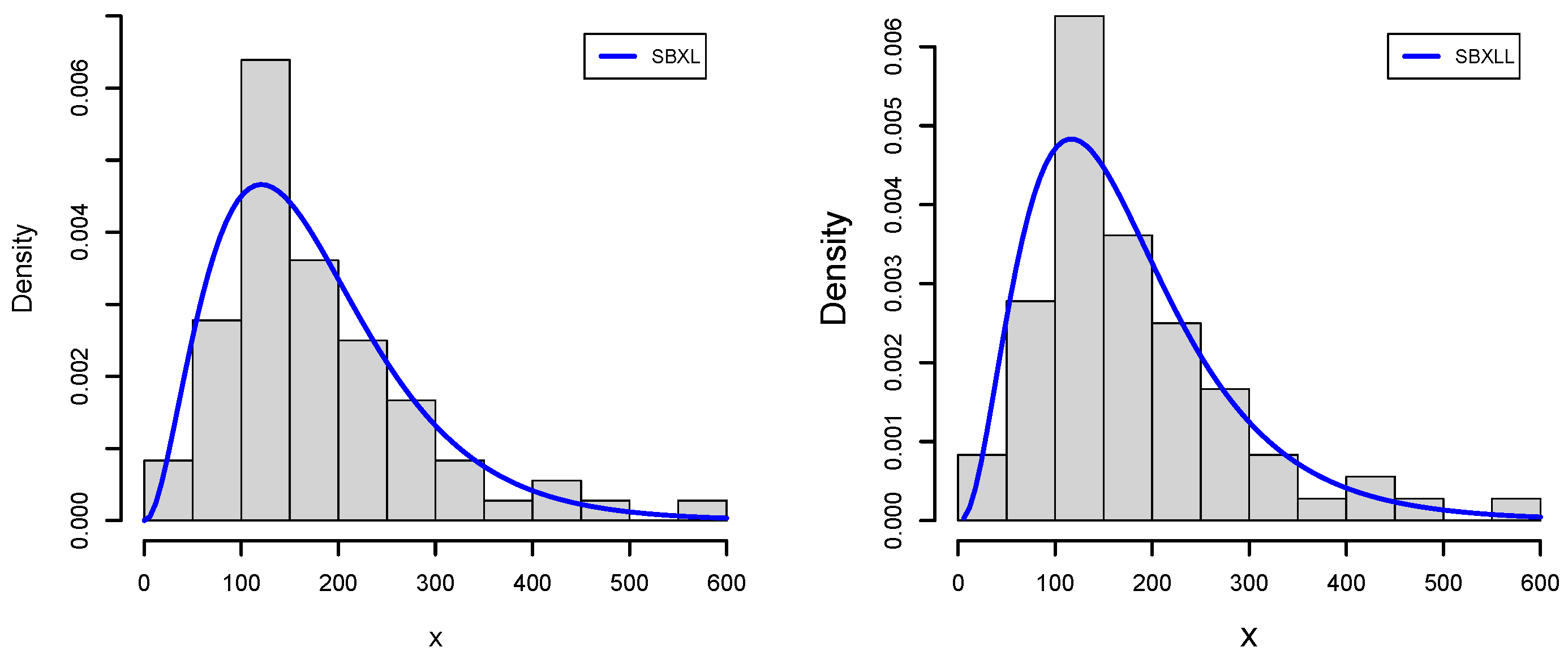
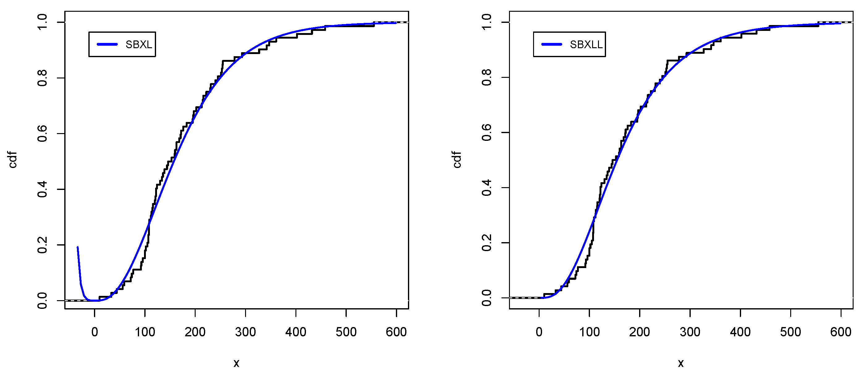
Case-I: Environmental Data Sets
Any occurrence, activity, or state that has a harmful effect on the environment is considered an environmental hazard. Physical or chemical pollution in the air, water, and soil is a reflection of environmental risks. Environmental risks have the ability to damage both people and the environment severely. There is a growing global effort to enhance environmental-related decision-making.
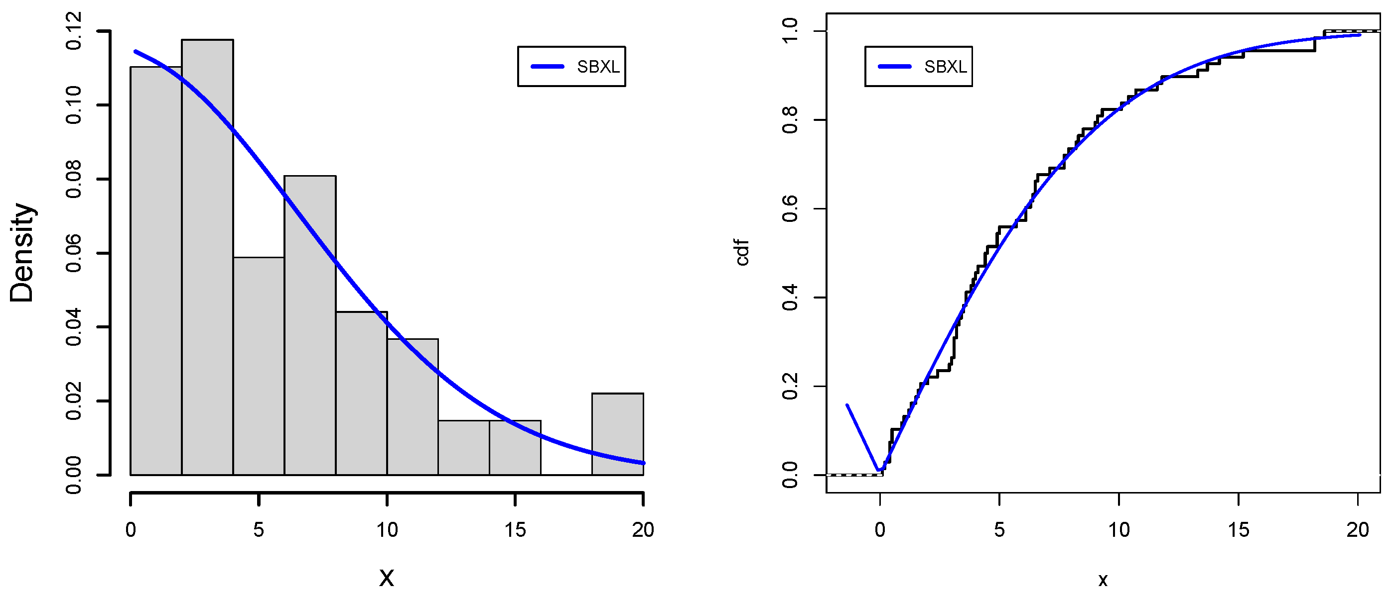
Data-I. Because of the large concentrations of nitric and sulfuric acids in the atmosphere that are washed down to the earth, acid rain is a common environmental phenomenon that has a trickle-down effect on a number of ecological variables, such as numbers of species, abundances of worms, change in the sizes of crabs, measures of quality of water or physiological condition of individual animals, etc. The production of acidic pollutants in the atmosphere results from the oxidation of sulpher and nitrogen in coal and other fossil fuels. In many industrialized nations, acid rain has significantly harmed forests. Acid rain can be avoided by using low-sulfur fuel and coal. Environmental catastrophes are covered in this part of the study. Acidity level is measured on a pH scale, which varies from one (highly acidic) to seven (neutral). Acid rain is considered to have a pH of less than 5.7. The first data measures the acidity of rainfalls for forty days in the state of Minnesota. This data set was reported by [52], and its values are given as 3.71, 4.23, 4.16, 2.98, 3.23, 4.67, 3.99, 5.04, 4.55, 3.24, 2.80, 3.44, 3.27, 2.66, 2.95, 4.70, 5.12, 3.77, 3.12, 2.38, 4.57, 3.88, 2.97, 3.70, 2.53, 2.67, 4.12, 4.80, 3.55, 3.86, 2.51, 3.33, 3.85, 2.35, 3.12, 4.39, 5.09, 3.38, 2.73, 3.07. In addition, for drawing a valid conclusion, grouping of the data is made via the R computational package. Possible groups, [0.03, 2.54], [2.54, 6.22], [6.22, 11.8], [11.8, 21.7], [21.7, 38.7], [38.7, 60.6], possess the frequencies 9, 8, 8, 8, 8, 9, respectively.
Table 5 and Table 6 show that there is a close association between theoretical and descriptive statistics of data. It also implies that the proposed model has an ability to work in platykurtic and positively skewed data much more effectively as compared to the competing distributions.
Furthermore, Table 7 and Table 8 exhibit the environment, which supports the proposed model in every aspect. These tables not only display that SBXL has the least values of goodness of fit statistics but also the minimum loss of information principle.
Data-II (Table 9). In order to simulate detectability, distances of observed targets from transect lines are frequently utilized in line-transect distance sampling to estimate population densities. The present crisis is associated with large populations of wild animals in a particular environment. This method’s fundamental premise is that all creatures are found where they first appear. Thus, animal migration that is not controlled by the transect and observer might seriously disrupt the natural food chain in a community. This data set, obtained from [53], represents the distances from the transect line for the 68 stakes detected in walking L = 1000 m and searching w = 20 m on each side of the line. The measurements are: 2.0, 0.5, 10.4, 3.6, 0.9, 1.0, 3.4, 2.9, 8.2, 6.5, 5.7, 3.0, 4.0, 0.1, 11.8, 14.2, 2.4, 1.6, 13.3, 6.5, 8.3, 4.9, 1.5, 18.6, 0.4, 0.4, 0.2, 11.6, 3.2, 7.1, 10.7, 3.9, 6.1, 6.4, 3.8, 15.2, 3.5, 3.1, 7.9, 18.2, 10.1, 4.4, 1.3, 13.7, 6.3, 3.6, 9.0, 7.7, 4.9, 9.1, 3.3, 8.5, 6.1, 0.4, 9.3, 0.5, 1.2, 1.7, 4.5, 3.1, 3.1, 6.6, 4.4, 5.0, 3.2, 7.7, 18.2, 4.1. For converting into groups, the bins code of the R computational package is used, and possible groups with respective frequencies are displayed as [0.1, 1.52], [1.52, 3.23], [3.23, 4.45], [4.45, 6.57], [6.57, 9.97], [9.97, 18.6], and the frequencies are 12, 11, 11, 11, 11 and 12, respectively.
Table 10 and Table 11 also advocate that SBXL explains the data situation in a better manner. However, the tune of working the SBXL is encouraging in that it not only works in positively skewed data but also has the strength to manage the lepto kurtic curves in a better fashion as compared with the competing distributions.
Moreover, Table 12 and Table 13 represent that the SBXL model and the data conditions are very well by showing the minimum values of χ 2 and the highest p-value of KS statistics alongside the least values of A D 0 * and C V M 0 * .
Overall Analysis of Data set-I and II via Goodness of Fit: Table 7 and Table 8 indicate that the proposed model exhibits much better goodness of fit statistics values compared with the competing distribution. However, some silent features are worth mentioning, such as chi-square ( χ 2 ) , A 0 * , and W 0 * , and KS values are the least among the competing models along with the highest p-value; thus, the mentioned tables totally support the suitability of the proposed model. Further, Table 9 further consolidates our claim of the suitability of a larger Vuong test statistics value. In addition, the proposed model also openly displays its suitability for data set II in which Table 12 and Table 13 exhibit the minimum values of chi-square ( χ 2 ) and A 0 * . Additionally, Table 14 suggests that the proposed model is the only model with reliable Vuong statistics. Overall, Table 8 and Table 13 suggest that the proposed model also possesses the minimum values of log-likelihood ( l ) and all the other information criteria, especially when compared to its competing four-parameter and three-parameter distributions asserting the acclaimed supremacy.
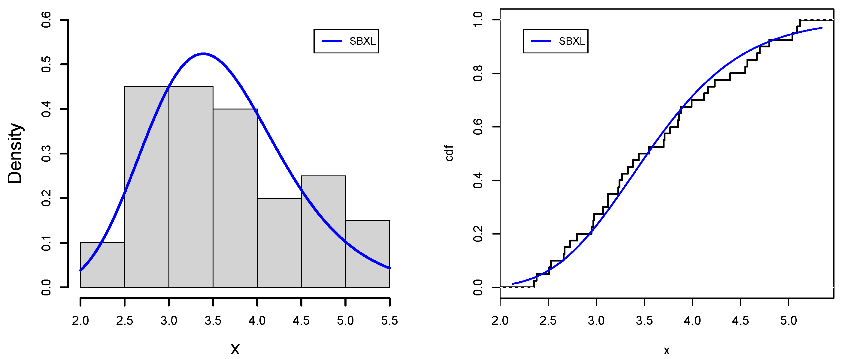
Figure 7, Figure 8, Figure 9 and Figure 10 support the numerical values results of the application for data sets I and II, respectively, which strengthen our claim regarding the dominance of the SBXL model over its respective competitive models.
Case-II: Failure time data sets
Failure is the occurrence, or unsuitable state, in which any object or component of an item does not or would not operate as previously defined. Failure analysis is the logical, systematic investigation of a product, its design, use, and documentation after a failure in order to pinpoint the failure mode, pinpoint the failure mechanism, and pinpoint the failure’s fundamental cause. As systems are becoming more diverse, failure time analysis is a discipline whose significance continues to expand. In the subsection under study, we explore two data sets that are related to this field.
Data-III: The braking system on a vehicle defines the safety of the vehicle. The brake pads and disk setup make up the braking system, where the brake pads are critical safety components see [27]. In this regard, a manufacturer decided to select a sample of vehicles sold over the preceding 12 months at a specific group of dealers. After that period, only the cars that still had the initial pads were reselected. For each car, the brake pad failure time measurement x i could have been observed. In this regard, the following data represent the failure time of automobile brake pads for 98 cars, where the number of miles or kilometers are driven is known to be related to the pads failure time; see [50]. However, the current data only present the failure time x i (in km) data, which is left truncated; see [47]. In addition, for drawing a valid conclusion, we have created different classes, such as [18.6, 44], [44, 53.9], [53.9, 65], [65, 77.6], [77.6, 91], [91, 166], having a number of observations against each class, which are 15, 15, 14, 15, 14, 15, respectively.
Table 15 and Table 16 also reinforce that SBXLL explains the data situation in a nice way. However, the theoretical values of mean, median, standard deviation, skewness and kurtosis are in accordance with its observed facts. Further, the tune of working the SBXLL is encouraging in that it not only works in positively skewed data but also has the strength to manage the lepto kurtic curves in a better fashion compared with its competing distributions (Table 17 and Table 18).
Furthermore, the VT statistics, as displayed in Table 19, are also in close association with the above results. Thus, our proposed model seems to be a natural choice for such data sets.
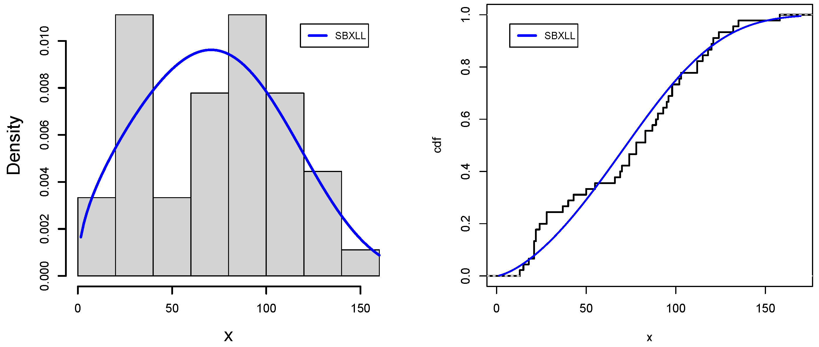
Data IV: A power failure is a period of time during which the electricity supply to a specific structure or area is interrupted, typically as a result of a natural weather event, such as damage to the cables caused by strong winds, lightning, freezing rain, ice buildup on the lines, snow, etc. Power outages can also be triggered by wildlife and tree branches hitting power cables. This data set is obtained from [29] the power failures’ lengths measured in minutes: 22, 18, 135, 15, 90, 78, 69, 98, 102, 83, 55, 28, 121, 120, 13, 22, 124, 112, 70, 66, 74, 89, 103, 24, 21, 112, 21, 40, 98, 87, 132, 115, 21, 28, 43, 37, 50, 96, 118, 158, 74, 78, 83, 93, 95. We have also grouped the data with the help of the bins code of the R computational package, where possible classes with respective frequencies are enlisted as [13, 22.7], [22.7, 53.3], [53.3, 78], [78, 95.3], [95.3, 114], [114, 158] and frequencies are 8,7,8, 7,7 and 8, respectively (Table 20 and Table 21).
Moreover, Table 22 and Table 23 offer that the SBXLL models and the data conditions are very well by showing the minimum values of χ 2 and highest p-value of KS statistics along with the lowest values of A D 0 * C V M 0 * , as well as the lowest loss of information behavior.
Furthermore, the VT statistics, as displayed in Table 24, are in close association with the above results. Thus, our proposed model seems to be a natural choice for such data sets.
General discussion about data set-III and IV: Table 15 and Table 16 show that data set-III is positively skewed; however, Table 20 and Table 21 related to data set-IV exhibit a negatively skewed behavior of platykurtic nature. In addition, both data sets are in a non-normal phenomenon, which is tested by the Shapiro–Wilk test and found to be non-normal with the Shapiro–Wilk test statistics 0.9603 and 0.9455 with p-values 0.0087 and 0.0342, respectively. Furthermore, for outlier detection, Grubbsťest is used, which indicates that data set-III shows some evidence of outlier presence with critical values of Z = 3.3399 , whereas data set-IV does not produce any sign of outliers with Z = 3.0854 at the 5% level of significance.
Analysis of Data set-III and IV via Goodness of Fit: From Table 17, Table 18, Table 22 and Table 23, it is quite evident that the proposed model yielded much better goodness of fit statistics as compared to its competing distributions. These statistics completely outfit the competing models in all respects. Further, minimum χ 2 outweighs the VT statistic value in Table 19 and Table 24, which paves the path of suitability of the proposed model. Figure 11 and Figure 12 support the numerical value results of applications for data sets III and IV, respectively, which further solidifies the superiority of SBXLL models over the competitive models.
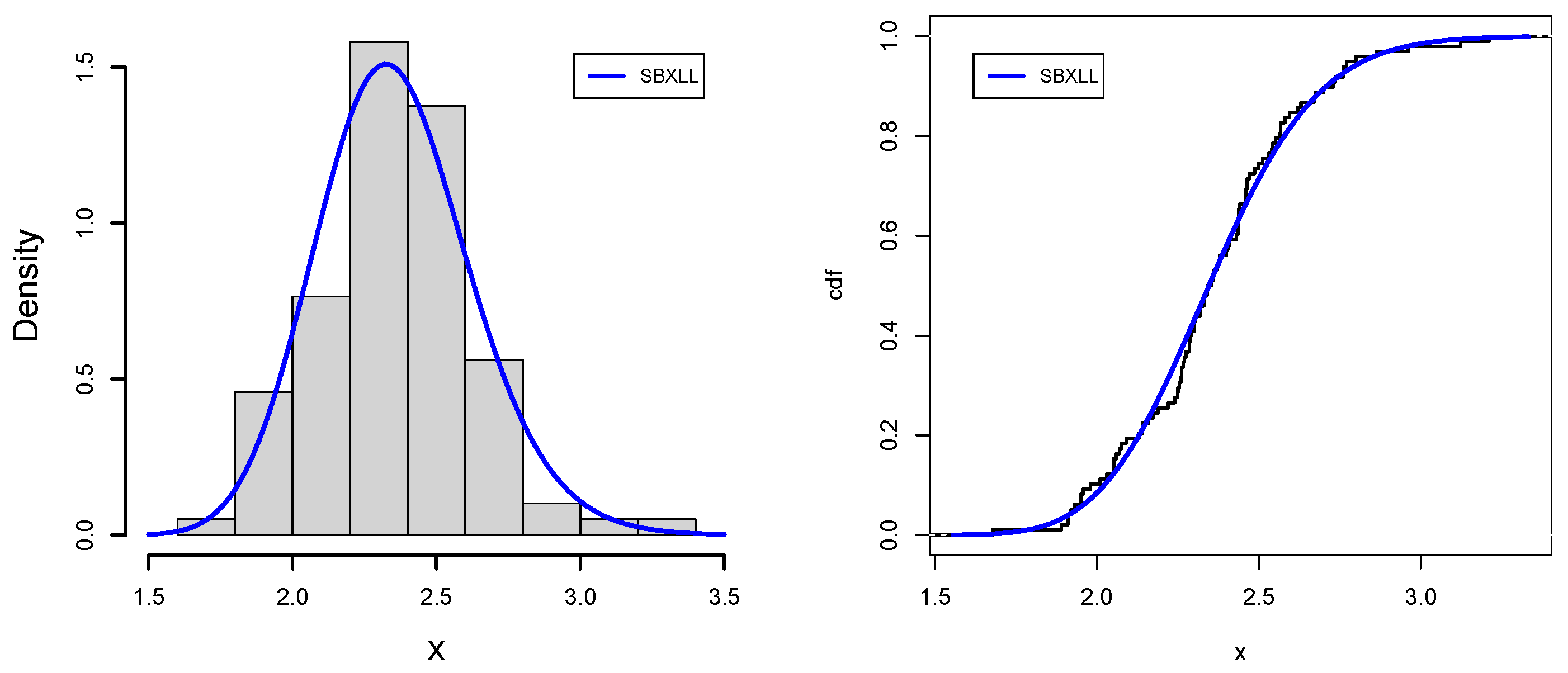
Case-III: Biomedical Data Set
Data-V One of the most serious bacterial diseases in the world is mycobacterial tuberculosis (MBT). MBT infection affects two billion people, according to estimates. Since MTB is easily transmitted and long-course chemotherapy treatments are challenging to deliver, controlling the disease is a daunting task. Developing short-term antibiotic regimens to reduce the emergence of drug resistance, developing novel medications to treat TB patients, and developing new vaccines with more efficacy than traditional vaccines, such as BCG, are all critically needed new methods for the control of TB. Organs and tissues from guinea pigs are typically utilized in scientific research. Guinea pig blood transfusions and isolated organ preparations, including lung and intestine from the species, are extensively used in studies to develop novel drugs. The fifth data set corresponds to the survival time of the guinea pigs after receiving an injection of a specific amount of MBT in a medical experiment, as recently studied by [54] in the context of comparative parameter estimation techniques. some descriptive measures of the data are reported in Table 25.
The descriptive statistics reveal that data-V has a right-tailed distribution. A higher σ ^ signifies more varied results when MBT is infused into the bloodstream of guinea pigs. This variability is evident from the kurtosis result of platykurtic characteristics. The result in Table 26 shows that both special models, SBXL and SBXLL, have similar properties to fit data of this nature.
Moreover, Table 27 and Table 28 represent that for SBXL and SBXLL models, the data are displayed very well by showing minimum values of χ 2 , the highest p-value of KS statistics, and the lowest values of AD 0 * and CVM 0 * , as well as the lowest loss of information behavior.
Furthermore, the VT statistics as displayed in Table 29 are closely related to the above results. These results suggest that the proposed model (SBXL) seems to be more appropriate for such data set.
The comparison of VT statistics, presented in Table 30, reasserts the superior behaviour of the proposed SBXLL for the data set.
Analysis of Data set-V via Goodness of Fit: The empirical findings in Table 27 and Table 28 are quite revealing of the fact that the proposed models, SBXL and SBXLL, yield far better goodness of fit statistics than its parallel models. Moreover, the minimum χ 2 is significant to the VT statistic value in Table 29 and Table 30, which further strengthens the suitability of the proposed model. Figure 11 and Figure 12 support the evaluated results of application for data set V, which further solidifies the superiority of SBXL and SBXLL models over well-established competing models.

7. Conclusions

This article presents a new family under the name Sine Burr X G family of distributions. Some properties of the proposed family such as moments and moment generating function, percentile function, partial moments, order statistics, Lorenz and Bonferroni Curves and mean deviance are discussed. The model parameters are estimated by the MLE method. Four members of Sine Burr X G are considered, including Sine Burr X Lomax, Sine Burr X exponential, Sine Burr X Rayleigh and Sine Burr X log-logistic distribution. Environmental, failure life testing and biomedical experimental data sets are modeled via Sine Burr X Lomax and Sine Burr X log-logistic models on four different data sets. In each case, the proposed models produced reliable results while observing the least lost information principles. The fact that the special models stemmed from the proposed generalization are flexible enough to model data sets from such a diverse field makes it a quintessential family for further exploration. To be more concise, we are hopeful that the proposed family, along with its members, will be appealing for extensive applications in numerous fields such as insurance, bio-informatics, economics and queuing theory, as well as meteorology and hydrology.

Author Contributions

Conceptualization, I.E. and M.E.; methodology, H.E.S.; software, S.K.; validation, M.M.A., T.H. and N.A.; formal analysis, S.K. and T.H.; investigation, N.A.; resources, H.E.S.; writing—original draft preparation, M.E. and I.E.; writing—review and editing, M.E., S.K. and I.E.; visualization, N.A.; supervision, N.A.; project administration, H.E.S.; funding acquisition, I.E. All authors have read and agreed to the published version of the manuscript.

Funding

The authors extend their appreciation to the Deputyship for Research & Innovation, Ministry of Education in Saudi Arabia for funding this research work through project number IFP-IMSIU202203.

Data Availability Statement

All the data sets are readily available in the manuscript.

Conflicts of Interest

The authors declare no conflict to interest.

References

  1. Marshall, A.; Olkin, I. A new method for adding a parameter to a family of distributions with applications to the exponential and Weibull families. Biometrika 1997, 84, 641–652. [Google Scholar] [CrossRef]
  2. Eugene, N.; Lee, C.; Famoye, F. Beta-normal distribution and its applications. Commun. Stat. Theory Methods 2002, 31, 497–512. [Google Scholar] [CrossRef]
  3. Cordeiro, G.; de Castro, M. A new family of generalized distributions. J. Stat. Comput. Simul. 2011, 81, 883–898. [Google Scholar] [CrossRef]
  4. Haq, M.; Elgarhy, M. The odd Fréchet- G family of probability distributions. J. Stat. Appl. Probab. 2018, 7, 189–203. [Google Scholar] [CrossRef]
  5. Torabi, H.; Montazeri, N.H. The logistic-uniform distribution and its application. Commun. Stat. Simul. Comput. 2014, 43, 2551–2569. [Google Scholar] [CrossRef]
  6. Cordeiro, G.; Ortega, E.; da Cunha, D.C. The exponentiated generalized class of distributions. J. Data Sci. 2013, 11, 1–27. [Google Scholar] [CrossRef]
  7. Zubair, A.; Elgarhy, M.; Hamedani, G.; Butt, N. Odd generalized N-H generated family of distributions with application to exponential model. Pak. J. Stat. Oper. Res. 2020, 16, 53–71. [Google Scholar]
  8. Alzaatreh, A.; Lee, C.; Famoye, F. A new method for generating families of continuous distributions. Metron 2013, 71, 63–79. [Google Scholar] [CrossRef] [Green Version]
  9. Badr, M.M.; Elbatal, I.; Jamal, F.; Chesneau, C.; Elgarhy, M. The transmuted odd Fréchet-G family of distributions: Theory and applications. Mathematics 2020, 8, 958. [Google Scholar] [CrossRef]
  10. Aldahlan, M.A.; Jamal, F.; Chesneau, C.; Elbatal, I.; Elgarhy, M. Exponentiated power generalized Weibull power series family of distributions: Properties, estimation and applications. PLoS ONE 2020, 15, e0230004. [Google Scholar] [CrossRef] [Green Version]
  11. Bourguignon, M.; Silva, R.B.; Cordeiro, G.M. The Weibull-G family of probability distributions. J. Data Sci. 2014, 12, 1253–1268. [Google Scholar] [CrossRef]
  12. Cordeiro, G.; Alizadeh, M.; Ortega, E. The exponentiated half-logistic family of distributions: Properties and applications. J. Probab. Stat. 2014, 81, 1–21. [Google Scholar] [CrossRef]
  13. Hassan, A.S.; Elgarhy, M.; Shakil, M. Type II half Logistic family of distributions with applications. Pak. J. Stat. Oper. Res. 2017, 13, 245–264. [Google Scholar]
  14. El-Sherpieny, E.S.A.; Muhammed, H.Z.; Almetwally, E.M. Bivariate Weibull-G family based on copula function: Properties, Bayesian and non-Bayesian estimation and applications. Statistics. Optim. Inf. Comput. 2022, 10, 678–709. [Google Scholar] [CrossRef]
  15. ElSherpieny, E.A.; Almetwally, E.M. The Exponentiated Generalized Alpha Power Family of Distribution: Properties and Applications. Pak. J. Stat. Oper. Res. 2022, 8, 349–367. [Google Scholar] [CrossRef]
  16. Alotaibi, N.; Elbatal, I.; Almetwally, E.M.; Alyami, S.A.; Al-Moisheer, A.S.; Elgarhy, M. Truncated Cauchy Power Weibull-G Class of Distributions: Bayesian and Non-Bayesian Inference Modelling for COVID-19 and Carbon Fiber Data. Mathematics 2022, 10, 1565. [Google Scholar] [CrossRef]
  17. Elbatal, I.; Alotaibi, N.; Almetwally, E.M.; Alyami, S.A.; Elgarhy, M. On Odd Perks-G Class of Distributions: Properties, Regression Model, Discretization, Bayesian and Non-Bayesian Estimation, and Applications. Symmetry 2022, 14, 883. [Google Scholar] [CrossRef]
  18. Algarni, A.; MAlmarashi, A.; Elbatal, I.; SHassan, A.; Almetwally, E.M.; MDaghistani, A.; Elgarhy, M. Type I half logistic Burr XG family: Properties, Bayesian, and non-Bayesian estimation under censored samples and applications to COVID-19 data. Math. Probl. Eng. 2021, 2021, 5461130. [Google Scholar] [CrossRef]
  19. Al-Babtain, A.A.; Elbatal, I.; Chesneau, C.; Elgarhy, M. Sine Topp-Leone-G family of distributions: Theory and applications. Open Phys. 2020, 18, 74–593. [Google Scholar] [CrossRef]
  20. Bantan, R.A.; Chesneau, C.; Jamal, F.; Elgarhy, M. On the Analysis of New COVID-19 Cases in Pakistan Using an Exponentiated Version of the M Family of Distributions. Mathematics 2020, 8, 953. [Google Scholar] [CrossRef]
  21. Bantan, R.A.; Jamal, F.; Chesneau, C.; Elgarhy, M. A New Power Topp–Leone Generated Family of Distributions with Applications. Entropy 2019, 21, 1177. [Google Scholar] [CrossRef] [Green Version]
  22. Bantan, R.A.; Jamal, F.; Chesneau, C.; Elgarhy, M. Truncated inverted Kumaraswamy generated family of distributions with applications. Entropy 2019, 21, 1089. [Google Scholar] [CrossRef] [Green Version]
  23. Tahir, M.H.; Cordeiro, G.M.; Alzaatreh, A.; Mansoor, M.; Zubair, M. The Logistic-X family of distributions and its applications. Commun. Stat.-Theory Methods 2016, 45, 7326–7349. [Google Scholar] [CrossRef] [Green Version]
  24. Cordeiro, G.M.; Alizadeh, M.; Tahir, H.; Mansoor, M.; Bourguignon, M.; Hamedani, G. The beta odd log-logistic family of distributions. Hacet. J. Math. Stat. 2015, forthcoming. [Google Scholar] [CrossRef]
  25. Mahdavi, A.; Kundu, D. A new method for generating distributions with an application to exponential distribution. Commun. Stat.-Theory Methods 2017, 46, 6543–6557. [Google Scholar] [CrossRef]
  26. Elbatal, I.; Aryal, G. A new generalization of the exponential Pareto distribution. J. Inf. Optim. Sci. 2017, 38, 675–697. [Google Scholar] [CrossRef]
  27. Elbatal, I.; Altun, E.; Afify, A.Z.; Ozel, G. The Generalized Burr XII Power Series Distributions with Properties and Applications. Ann. Data Sci. 2018, 6, 571–597. [Google Scholar] [CrossRef]
  28. Elbatal, I.; Mansour, M.M.; Ahsanullah, M. The Additive Weibull-Geometric Distribution: Theory and Applications. J. Stat. Theory Appl. 2016, 15, 125–141. [Google Scholar] [CrossRef] [Green Version]
  29. Shahzad, M.N.; Ullah, E.; Hussanan, A. Beta Exponentiated Modified Weibull Distribution: Properties and Application. Symmetry 2019, 11, 781. [Google Scholar] [CrossRef] [Green Version]
  30. Kumar, D.; Singh, U.; Singh, S.K. A New Distribution Using Sine Function Its Application to Bladder Cancer Patients Data. J. Stat. Appl. Probab. 2015, 4, 417–427. [Google Scholar]
  31. Nadarajah, S.; Kotz, S. Beta Trigonometric Distribution. Port. Econ. J. 2006, 5, 207–224. [Google Scholar] [CrossRef]
  32. Al-Faris, R.Q.; Khan, S. Sine Square Distribution: A New Statistical Model Based on the Sine Function. J. Appl. Probab. Stat. 2008, 3, 163–173. [Google Scholar]
  33. Raab, D.H.; Green, E.H. A cosine approximation to the normal distribution. Psychometrika 1961, 26, 447–450. [Google Scholar] [CrossRef]
  34. Kharazmi, O.; Saadatinik, A.; Jahangard, S. Odd Hyperbolic Cosine Exponential-Exponential (OHC-EE) Distribution. Ann. Data Sci. 2019, 6, 765–785. [Google Scholar] [CrossRef] [Green Version]
  35. Kharazmi, O.; Saadatinik, A.; Alizadeh, M.; Hamedani, G.G. Odd hyperbolic cosine-FG (OHC-FG) family of lifetime distributions. J. Stat. Appl. 2018, 18, 387–401. [Google Scholar]
  36. Bleed, S.; Abdelali, A. Transmuted Arcsine Distribution Properties and Application. Int. J. Res. 2018, 10, 1–11. [Google Scholar] [CrossRef]
  37. Wenjing, H.; Afify, Z.; Goual, H. The Arcsine Exponentiated-X Family: Validation and Insurance Application. Complexity 2020, 2020, 8394815. [Google Scholar] [CrossRef]
  38. Yousof, H.M.; Ahmed, Z.; Hamedani, G.H.; Aryal, G. The Burr X generator of distributions for lifetime data. J. Stat. Theory Appl. 2016, 16, 1–19. [Google Scholar] [CrossRef] [Green Version]
  39. Fayomi, A.; Khan, S.; Tahir, M.H.; Algarni, A.; Jamal, F.; Abu-Shanab, R. A New Extended Gumbel distribution: Properties and Application. PloS ONE 2022, 17, e0267142. [Google Scholar] [CrossRef]
  40. Lee, C.; Famoye, F.; Olumolade, O. Beta-Weibull Distribution: Some Properties and Applications to censored Data. J. Mod. Appl. Stat. Methods 2007, 6, 17. [Google Scholar] [CrossRef]
  41. Rajab, M.; Aleem, M.; Nawaz, T.; Daniyal, M. On Five Parameter Beta Lomax Distribution. J. Stat. 2013, 20, 102–118. [Google Scholar]
  42. Mead, M.E. On Five-Parameter Lomax Distribution:Properties and Applications. Pak. J. Stat. Oper. Res. 2015, 12, 185–199. [Google Scholar] [CrossRef]
  43. Cordeiro, G.M.; Ortega, E.M.M.; Ramires, T.G. A new generalized Weibull family of distributions: Mathematical properties and applications. J. Stat. Distrib. Appl. 2015, 2, 13. [Google Scholar] [CrossRef] [Green Version]
  44. Pal, M.; Ali, M.M.; Woo, J. Exponentiated Weibull distribution. Statistica 2006, 66, 139–147. [Google Scholar] [CrossRef]
  45. Mahmood, Z.; Chesneau, C. A New Sine-G Family of Distributions: Properties and Applications. Bull. Comput. App. Math. 2019, 7, 53–81. [Google Scholar]
  46. Gupta, R.D.; Kundu, D. Generalized exponential distribution. Austral N. Z. J. Stat. 1999, 41, 173–188. [Google Scholar] [CrossRef]
  47. Nadarajah, S.; Bakouch, H.S.; Tahmasbi, R. A generalized Lindley distribution. Sankhya B 2011, 73, 331–359. [Google Scholar] [CrossRef]
  48. Chesneau, C.; Bakouch, H.S.; Hussain, T.; Para, B.A. The cosine geometric distribution with count data modeling. J. Appl. Stat. 2021, 48, 124–137. [Google Scholar] [CrossRef]
  49. Hussain, T.; Bakouch, H.S.; Chesneau, C. A new probability model with application to heavy-tailed hydrological data. Environ. Ecol. Stat. 2019, 26, 12–151. [Google Scholar] [CrossRef]
  50. Hussain, T.; Bakouch, H.S.; Iqbal, Z. A New Probability Model for Hydrologic Events: Properties and Applications. J. Agric. Environ. Stat. 2018, 23, 63–82. [Google Scholar] [CrossRef]
  51. Vuong, Q.H. Likelihood ratio tests for model selection and non-nested hypotheses. Econometrica 1989, 57, 307–333. [Google Scholar] [CrossRef] [Green Version]
  52. Ross, M.S. Introductory Statistics, 3rd ed.; Elsevier: Oxford, UK, 2010; p. 365. [Google Scholar]
  53. Patil, G.P.; Rao, C.R. Handbook of Statistics 12: Environmental Statistics; Elsevier Science: Amsterdam, The Netherlands, 1994; p. 35. [Google Scholar]
  54. Mukherjee, I.; Maiti, S.S.; Singh, V.V. Study on estimators of the PDF and CDF of the one parameter polynomial exponential distribution. arXiv 2020, arXiv:2006.06272v1. [Google Scholar]
Figure 1. Pdf graphs of the SBXL model.
Axioms 11 00361 g001
Figure 2. Pdf graphs of the SBXLL model.
Axioms 11 00361 g002
Figure 3. Plots of hrf of the SBXL model for random parameter values.
Axioms 11 00361 g003
Figure 4. Plots of hrf of the SBXLL model for random parameter values.
Axioms 11 00361 g004
Figure 5. Three-dimensional plots of M ( X ) , V a r ( x ) , C S ( x ) and C K ( x ) of the SBXL distribution for β = 0.5 .
Axioms 11 00361 g005
Figure 6. Three-dimensional plots of M ( X ) , V a r ( x ) , C S ( x ) and C K ( x ) of the SBXLL distribution for θ = 0.5 .
Axioms 11 00361 g006
Figure 7. Plots of estimated pdf and cdf of the SBXL model for data set-I.
Axioms 11 00361 g007
Figure 8. Plots of estimated pdf and cdf of the SBXL model for data set-II.
Axioms 11 00361 g008
Figure 9. Plots of estimated pdf and cdf of the SBXLL model for data set-III.
Axioms 11 00361 g009
Figure 10. Plots of estimated pdf and cdf of the SBXLL model for data set-IV.
Axioms 11 00361 g010
Figure 11. Plots of estimated pdf of SBXL and SBXLL models for data set V.
Axioms 11 00361 g011
Figure 12. Plots of estimated cdf of SBXL and SBXLL models for data set V.
Axioms 11 00361 g012
Table 1. Odds ratios and baseline models.
Model cdf pdf G ¯ ( x ; δ ) G ( x ; δ ) 1
Lomax 1 ( β + x β ) α α β ( β + x β ) α 1 ( β β + x ) α 1
Log-logistic x β θ + x β β θ x β 1 θ + x β θ x 2 β
Exponential e μ x 1 e μ x μ e μ x e μ x 1
Rayleigh e ρ 2 x 2 1 e ρ 2 x 2 ρ x e ρ 2 x 2 e ρ 2 x 2 1
Table 2. Numerical values of M ( X ) , V a r ( x ) , C S ( x ) , C K ( x ) , and C V ( x ) at β = α = 0.5 for the SBXL model.
θ M   ( X ) Var   ( x ) CS   ( x ) CK   ( x ) CV   ( x )
0.50.5390.2391.6386.7460.908
1.00.9460.3471.0884.6770.623
1.51.2280.3910.8924.1780.51
2.01.4390.4120.7933.9760.446
2.51.6090.4230.7343.8740.404
3.01.7490.4290.6953.8140.375
3.51.8690.4320.6683.7760.352
4.01.9730.4340.6483.7510.334
4.52.0650.4350.6333.7340.319
5.02.1480.4350.6223.7210.307
Table 3. Numerical values of M ( X ) , V a r ( x ) , C S ( x ) , C K ( x ) , and C V ( x ) at β = α = 0.5 for the SBXLL model.
θ M   ( X ) Var   ( x ) CS   ( x ) CK   ( x ) CV   ( x )
0.50.060.012.96415.5961.686
1.00.1370.0211.737.3491.067
1.50.2060.0281.3035.6350.814
2.00.2660.0311.1545.1910.662
2.50.320.0311.2085.1870.553
3.00.3680.0291.5055.2990.467
3.50.4110.0262.1995.1550.393
4.00.450.0213.7063.7750.326
Table 4. CDFs of proposed models.
Model F   ( x ; δ ) ParametersRange
S B X L sin 1 2 1 e 1 x + β β θ 2 x + β β 2 θ α π ( α , β , θ ) [ 0 , ]
S B X L L sin 1 2 1 e θ x 2 β α π ( α , β , θ ) [ 0 , ]
Table 5. Summary statistics related to data-I.
Sample Size Mean X ¯ Median X ˜ Standard Deviation σ ^ Skewness Kurtosis
40 3.6122 3.4954 0.8047 0.2859 2.0191
Table 6. Theoretical statistical measures from SBXL for data-I.
Sample Size Mean X ¯ Median X ˜ Standard Deviation σ ^ Skewness Kurtosis
40 3.6218 3.5863 0.8000 0.2147 2.9618
Table 7. MLEs and goodness-of-fit of data set-I.
Models α ^ β ^ θ ^ γ ^ χ 2 AD 0 * CVM 0 * KS PV   ( KS )
S B X L 30.5303 0.2224 0.3680 2.1195 0.3637 0.0485 0.0799 0.9646
B W D 0.0544 3.9609 4.5734 0.1019 3.0735 0.4249 0.0613 0.0885 0.9125
B L D 9.9575 25.9269 26.7723 10.5916 2.9953 0.3708 0.0604 0.0877 0.9175
E G L D 7.7394 68.8101 13.7223 128.7546 2.8636 0.3832 0.0506 0.0894 0.9382
W G L D 11.0919 11.6079 0.3943 0.5703 4.3284 0.4893 0.0714 0.0930 0.8799
E W D 47.4928 0.0165 8.2713 3.0735 0.3801 0.0693 0.0806 0.9479
O W L D 18.9501 106.3052 3.6802 12.8453 0.6767 0.1027 0.1064 0.7554
N S I W 3.856600 3.266692 3.7349 0.3714 0.0548 0.0810 0.9511
E E D 2.6967 0.3382 38.6008 8.4487 1.6982 0.4087 0.0000
G L D 10.2202 1.0639 4.4707 1.5511 0.1871 0.1491 0.3512
W D 0.0023 4.4836 3.0735 0.5437 0.0805 0.1012 0.8077
L D 7.5284 3.5262 3.0226 0.4015 0.0529 0.0807 0.9474
L L D 6.7344 2.8703 2.9535 0.4117 0.0591 0.0901 0.9358
Table 8. Comparison of data set I fitting via information criterion.
Models A . I . C A . IC . C B . I . C H . Q . I . C
S B X L 47.0030 100.0057 100.6731 105.0733 96.6166
B W D 48.4137 100.8277 100.9970 106.5828 102.2698
B L D 48.8895 101.7009 102.8438 108.4564 104.1435
E G L D 47.5174 102.3141 103.4570 109.0696 104.7567
W G L D 47.6097 103.2195 104.3623 109.9750 105.6621
E W D 47.9585 100.9172 100.9983 104.9838 101.7491
O W L D 48.6081 103.2161 103.8828 108.2827 105.0481
N S I W 48.3782 101.0086 101.0461 102.0996 102.9495
E E D 77.7123 159.4251 159.7488 162.8020 158.0353
G L D 53.7586 111.5172 111.8424 114.8951 110.1278
W D 48.1185 100.2374 100.5613 103.6150 98.8476
L D 48.1807 102.3611 103.0284 107.4283 98.9725
L L D 49.0458 102.8763 103.6385 107.8823 97.8977
Table 9. Vuong’s test applied on data set-I at Z 0.05 = 1.6495 .
SBXL vs. Competitive ModelsVT Statistic
SBXL-BWD2.3761
SBXL-BLD2.8756
SBXL-EGLD3.5247
SBXL-WGLD4.2291
SBXL-EWD4.8345
SBXL-OWLD44.0316
SBXL-NSIWD2.0185
SBXL-EED30.4271
SBXL-GLD16.3573
SBXL-WD4.3604
SBXL-LD106.4452
SBXL-LLD112.2178
Table 10. Summary statistics of data-II.
Sample Size Mean X ¯ Median X ˜ Standard Deviation σ ^ Skewness Kurtosis
68 5.85294 4.45 4.61278 1.04362 3.57505
Table 11. Theoretical statistical measures from SBXL for data-II.
Sample Size Mean X ¯ Median X ˜ Standard Deviation σ ^ Skewness Kurtosis
68 5.8571 4.9382 4.5080 1.0116 3.5702
Table 12. MLEs and goodness-of-fit of data set-II.
Models α ^ β ^ θ ^ γ ^ χ 2 AD 0 * CVM 0 * KS PV   ( KS )
S B X L 0.4974 12.2054 0.8773 1.8984 0.2192 0.0387 0.0804 0.8692
B W D 0.6260 1.3917 0.5820 0.1062 3.4463 0.2362 0.0634 0.0868 0.6857
B L D 1.2714 0.0013 1.3149 0.0019 3.2564 0.4170 0.0638 0.1040 0.4533
E G L D 6.8051 220.0718 6.7324 1.3362 3.0277 0.4691 0.0717 0.1099 0.3846
W G L D 0.0750 1.2248 6.6913 3.3001 3.1158 0.3191 0.0487 0.0886 0.6592
E W D 0.0252 1.7046 0.5907 2.2251 0.2544 0.0397 0.0824 0.7445
O W L D 2.6063 21.4260 1.0227 2.4675 0.2597 0.0407 0.0835 0.7302
N S I W 0.6660 2.4866 2.3365 2.8257 0.4873 0.1975 0.0099
E E D 1.3143 0.2019 2.1244 0.5680 0.1111 0.1069 0.5562
G L D 10.2202 1.0639 1.9390 0.3317 0.0630 0.0846 0.8257
W D 1.2247 6.2368 1.9280 0.3651 0.0679 0.0876 0.7929
L D 5.6365 3.2990 3.0226 0.4214 0.0646 0.1554 0.0749
L L D 1.6846 4.3560 4.6666 0.9082 0.1238 0.0987 0.6577
Table 13. Comparison of data set II fitting via information criterion.
Models A . I . C A . IC . C B . I . C H . Q . I . C
S B X L 185.6611 377.3223 377.6968 383.9813 374.2013
B W D 185.9481 378.9963 379.6312 387.8743 382.5144
B L D 186.6941 381.3901 382.0253 390.2682 384.9079
E G L D 187.0306 382.0613 382.6962 390.9393 385.5787
W G L D 186.1698 380.3396 380.9746 389.2177 383.8574
E W D 186.6645 377.3291 377.7041 383.9876 379.9674
O W L D 185.8764 377.2975 377.6725 383.9564 379.9358
N S I W 200.7792 405.5584 405.7433 409.9974 407.3173
E E D 186.8347 377.6734 377.8553 382.1087 376.5494
G L D 186.1171 376.2343 376.4192 380.6734 375.1133
W D 186.1662 376.3386 376.5254 380.7787 375.2187
L D 188.5522 380.3044 380.4891 384.7434 382.0633
L L D 189.0323 379.9585 380.0578 385.5677 381.5556
Table 14. Vuong’s test (VT) applied on data set II at Z 0.05 = 1.6495 .
SBXL vs. Competitive ModelsVT Statistic
SBXL-BWD 2.7768
SBXL-BLD 2.3687
SBXL-EGLD 2.2256
SBXL-WGLD 2.9457
SBXL-EWD 4.3338
SBXL-OWLD 31.9597
SBXL-NSIWD 8.7761
SBXL-EED 14.7258
SBXL-GLD 8.5635
SBXL-WD 4.5416
SBXL-LD 10.4765
SBXL-LLD 13.2963
Table 15. Summary statistics in relation to data-III.
Sample Size Mean X ¯ Median X ˜ Standard Deviation σ ^ Skewness Kurtosis
88 68.1591 65.05 27.4718 0.8338 4.0272
Table 16. Theoretical statistical measures of SBXLL from data-III.
Sample Size Mean X ¯ Median X ˜ Standard Deviation σ ^ Skewness Kurtosis
88 68.2507 64.4438 27.2967 0.7650 3.9182
Table 17. Data set-III MLEs and goodness-of-fit.
Models α ^ β ^ θ ^ γ ^ χ 2 AD 0 * CVM 0 * KS PV   ( KS )
S B X L L 6.0813 0.5045 0.0268 0.9946 0.1045 0.0149 0.0315 0.9999
B W D 0.2517 2.7226 17.0036 1.7123 1.9937 0.4010 0.0683 0.0820 0.5247
B L D 15.5647 29.6341 91.7367 40.5312 1.5934 0.3995 0.0677 0.0816 0.5321
E G L D 80.1122 316.0927 15.6661 85.8891 1.7209 1.1802 0.2201 0.1255 0.0913
W G L D 4.5165 18.8058 0.5107 0.4862 1.8547 1.0757 0.1669 0.1006 0.2743
E W D 0.1496 3.4499 11.3889 1.6958 0.4071 0.0692 0.0822 0.5218
O W L D 0.2680 0.2018 17.4795 3.5842 1.1591 0.1804 0.1034 0.2458
N S I W 7.1975 2.2476 1.7896 0.8253 0.1523 0.1116 0.1741
E E D 7.7800 0.0391 2.5856 0.3967 0.0584 0.0595 0.9142
G L D 3.6472 0.0495 2.0576 0.2833 0.0409 0.0542 0.9584
W D 2.6364 76.7476 2.6992 0.4909 0.0633 0.0562 0.9443
L D 5.6365 3.2990 3.0226 0.4214 0.0646 0.1554 0.0749
L L D 4.2487 63.7755 1.6295 0.3365 0.0507 0.0657 0.7925
Table 18. Comparison of data set III fitting via information criterion.
Models A . I . C A . IC . C B . I . C H . Q . I . C
S B X L L 10.3317 26.6622 26.9175 34.4171 29.7989
B W D 10.4715 28.9431 29.3732 39.2830 33.1254
B L D 10.5156 29.0313 29.4614 39.3712 33.2136
E G L D 14.6995 37.3991 37.8291 47.7389 41.5813
W G L D 17.1390 42.2780 42.7081 52.6179 46.4603
E W D 10.4983 26.9966 27.2519 34.7515 30.1333
O W L D 17.8231 41.6462 41.9015 49.4011 44.7829
N S I W 12.7407 29.4813 29.6076 34.6512 31.5724
E E D 14.6706 33.3412 33.4675 38.5112 35.4324
G L D 14.4864 32.9729 33.0992 38.1428 35.0640
W D 23.6554 51.3108 51.4371 56.4807 53.4019
L D 10.6993 26.9987 26.9520 34.5686 29.9898
L L D 10.8453 27.1079 27.55420 35.5044 30.0577
Table 19. Vuong’s test applied on data set III at Z 0.05 = 1.6495 .
SBXLL vs. Competitive ModelsVT Statistic
SBXLL-BWD 15.4851
SBXLL-BLD 14.8878
SBXLL-EGLD 15.2235
SBXLL-WGLD 15.0976
SBXLL-EWD 12.4225
SBXLL-OWLD 12.2839
SBXLL-NSIWD 7.6190
SBXLL-EED 13.7947
SBXLL-GLD 25.1236
SBXLL-WD 14.6031
SBXLL-LD 21.2374
SBXLL-LLD 21.6273
Table 20. Summary statistics of data-IV.
Sample Size Mean X ¯ Median X ˜ Standard Deviation σ ^ Skewness Kurtosis
45 74.0222 78.2 39.2576 0.0320 1.9368
Table 21. Theoretical statistical measures of SBXLL from data-IV.
Sample Size Mean X ¯ Median X ˜ Standard Deviation σ ^ Skewness Kurtosis
45 73.7816 71.2079 37.8439 0.3305 2.5761
Table 22. MLEs and goodness-of-fit related to data set-IV.
Models α ^ β ^ θ ^ γ ^ χ 2 AD 0 * CVM 0 * KS PV   ( KS )
S B X L L 0.1629 4.4595 2.6685 0.9223 0.5494 0.1027 0.1201 0.6765
B W D 0.0763 1.2160 5.6457 0.0743 3.2255 0.4010 0.0683 0.1795 0.1099
B L D 25.1855 1.5357 2.7075 21.4818 5.6732 1.6030 0.2773 0.1586 0.2077
E G L D 0.0819 1.8119 17.7038 102.6406 4.2255 3.0921 0.5708 0.2286 0.0181
W G L D 4.5122 16.2195 0.1061 0.0153 3.7369 1.3633 0.2326 0.1390 0.3494
E W D 0.0068 1.2383 1.9409 2.6354 1.5627 0.2692 0.1589 0.2059
O W L D 0.0919 0.0436 10.1225 4.7582 1.3414 0.2284 0.1405 0.3365
N S I W 1.1473 47.9852 3.9768 2.6080 0.4739 0.2003 0.0540
E E D 2.8273 0.0238 5.1464 1.5958 0.3207 0.1844 0.1724
G L D 1.3903 0.0312 4.5330 1.5218 0.3067 0.1818 0.1849
W D 1.9781 83.4093 2.4573 1.1501 0.2210 0.1628 0.2960
L L D 2.4677 66.2694 1.6295 2.2040 0.3854 0.1471 0.2844
Table 23. Comparison of data set IV fitting via information criterion.
Models A . I . C A . IC . C B . I . C H . Q . I . C
S B X L L 225.0564 456.1122 456.6972 461.5322 452.7864
B W D 229.6199 467.2397 468.2397 474.4664 469.9338
B L D 229.0869 466.1738 467.1738 473.4005 468.8678
E G L D 238.1035 484.2072 485.2067 491.4336 486.9011
W G L D 227.9240 463.8945 464.8945 471.1211 466.5885
E W D 228.9637 463.9273 464.5127 469.3473 465.9478
O W L D 227.7871 461.5741 462.1595 466.9941 463.5947
N S I W 234.6733 473.3461 473.6317 476.9593 474.6935
E E D 229.8272 463.6544 463.9425 467.2670 462.3283
G L D 229.3441 462.6879 462.9743 466.3012 461.3622
W D 227.2559 458.5122 458.7977 462.1251 457.1862
L L D 233.4224 470.8121 471.0859 474.4133 469.4744
Table 24. Vuong’s test was applied on data set IV at Z 0.05 = 1.6495 .
SBXLL vs. Competitive ModelsVT Statistic
SBXLL-BWD 2.3032
SBXLL-BLD 1.9819
SBXLL-EGLD 2.6569
SBXLL-WGLD 3.3876
SBXLL-EWD 4.8703
SBXLL-OWLD 8.3492
SBXLL-NSIWD 6.4486
SBXLL-EED 9.0798
SBXLL-GLD 13.7117
SBXLL-WD 15.9164
SBXLL-LD 8.3895
SBXLL-LLD 6.7725
Table 25. Summary statistics of data-V.
Sample Size Mean X ¯ Median X ˜ Standard Deviation σ ^ Skewness Kurtosis
72 176.83 149.5 103.47 1.34 1.99
Table 26. Theoretical statistical measures of SBXL and SBXLL from data-V.
Sample Size Mean X Median X Standard Deviation σ Skewness Kurtosis
SBXL72 177.08 148.97 104.19 1.33 1.87
SBXLL72 176.11 149.35 103.67 1.38 2.01
Table 27. MLEs and goodness-of-fit related to data set-V for SBXL and SBXLL models.
Models α ^ β ^ θ ^ γ ^ χ 2 AD 0 * CVM 0 * KS PV   ( KS )
S B X L 0.3737 37.2369 1.6754 2.6003 0.5812 0.0941 0.0915 0.58
S B X L L 0.3574 72.5069 5.5707 2.5839 0.5226 0.0815 0.0904 0.60
B W D 0.0267 0.6894 6.4323 4.7862 2.8915 0.6352 0.1081 0.0955 0.54
B L D 0.2858 2003.3310 3.3293 138.3401 3.0317 0.6493 0.1097 0.0991 0.53
E G L D 0.8261 8.7069 1.1879 3.6286 3.2532 0.6213 0.1065 0.0932 0.56
W G L D 7.9726 13.7446 0.1129 0.0960 5.5278 0.7476 0.1238 0.1022 0.44
E W D 0.0138 0.9702 3.9882 3.1438 0.6177 0.1079 0.0950 0.54
O W L D 0.3446 30.0632 3.0396 5.2208 0.7044 0.1163 0.0982 0.49
N S I W 1.0842 112.8156 12.3261 1.7926 0.2602 0.1752 0.02
E E D 3.6485 0.0113 2.9243 0.6211 0.1080 0.0948 0.56
G L D 2.0117 89.2305 3.0125 0.6289 0.1096 0.0973 0.55
W D 0.0056 1.0027 2.9337 0.6072 0.1101 0.0955 0.56
L D 3.0116 152.385434 3.3120 0.6382 0.1056 0.0995 0.55
Table 28. Comparison of data set V fitting via information criterion of SBXL and SBXLL.
Models A . I . C A . IC . C B . I . C H . Q . I . C
S B X L 425.3818 857.6636 858.0165 864.4936 860.3826
S B X L 425.8595 857.7181 858.0720 864.5492 860.4381
B W D 426.1222 860.2443 860.8413 869.351 863.8697
B L D 426.7521 859.5043 860.1013 868.6109 863.1296
E G L D 425.8878 859.6356 860.2327 868.7423 863.2611
W G L D 426.4696 860.9393 861.5363 870.0459 864.5647
E W D 426.8178 859.6356 858.7435 864.9206 861.9096
O W L D 426.2470 859.4940 858.9469 865.324 861.2130
N S I W 438.5964 881.1928 881.3667 885.7461 883.0055
E E D 425.2054 858.5563 858.8103 865.1897 861.0091
G L D 444.6150 893.2300 893.4039 897.7833 895.0426
W D 444.6151 891.2299 891.2870 893.5066 892.1363
L D 426.0205 859.0125 858.9353 865.9778 861.0341
Table 29. Vuong’s test applied for the SBXL model on data set V at Z 0.05 = 1.6495 .
SBXL vs. Competitive ModelsVT Statistic
SBXL-BWD 2.2450
SBXL-BLD 2.1378
SBXL-EGLD 2.7656
SBXL-WGLD 3.2388
SBXL-EWD 2.5064
SBXL-OWLD 7.2364
SBXL-NSIWD 8.5946
SBXL-EED 2.1443
SBXL-GLD 10.4867
SBXL-WD 5.5667
SBXL-LD 6.1923
SBXL-LLD 6.2587
Table 30. Vuong’s test applied for the SBXLL model on data set V at Z 0.05 = 1.6495 .
SBXLL vs. Competitive ModelsVT Statistic
SBXLL-BWD 2.1315
SBXLL-BLD 2.2517
SBXLL-EGLD 2.5537
SBXLL-WGLD 3.1319
SBXLL-EWD 2.3503
SBXLL-OWLD 7.1204
SBXLL-NSIWD 8.4786
SBXLL-EED 2.1844
SBXLL-GLD 10.2237
SBXLL-WD 5.3935
SBXLL-LD 6.6912
SBXLL-LLD 5.7826
Publisher’s Note: MDPI stays neutral with regard to jurisdictional claims in published maps and institutional affiliations.

