On Implicit Time–Fractal–Fractional Differential Equation

Abstract

An implicit time–fractal–fractional differential equation involving the Atangana’s fractal–fractional derivative in the sense of Caputo with the Mittag–Leffler law type kernel is studied. Using the Banach fixed point theorem, the well-posedness of the solution is proved. We show that the solution exhibits an exponential growth bound, and, consequently, the long-time (asymptotic) property of the solution. We also give examples to illustrate our problem.

1. Introduction

The fractal–fractional differential equation is a link between the fractal and fractional differential equations. Fractal and fractional differential equations are known for modeling complex physical processes and phenomena, particularly irregular systems with memory. Although fractional equations are renowned for representing systems with long-term memory and long-range interactivity, fractal calculus, conversely, is immensely effective in working with occurrence in stratified or porous media. That is, fractal–fractional differential operator models physical phenomena and real-world activities that exhibit or display fractional behaviours (sponge-like media, aquifer, turbulence, etc.) namely finance, viscoelasticity, control theory, electrical networks, goundwater flow and geo-hydrology, wave propagation, plasma physics and fusion, rheology, chaotic processes, fluid mechanics and biological activities [1,2,3,4,5,6]. For more applications of fractal-fractional differential equations, see [7,8,9,10] and for recent results on fractional differential equations and their applications, see [11,12,13]. To explore more results on implicit fractional differential equations and their applications, see [14,15,16,17]. There are many results relating to implicit fractional differential equations in literature involving Caputo fractional derivatives both for initial value problems (IVP) and boundary value problems (BVP) [15,18,19,20,21].

In 2015, Benchohra and Souid in [18] studied the existence of integrable solutions for IVP for some given implicit fractional order functional differential equations with infinite delay

$$\begin{array}{c}\hfill \left\{\begin{array}{c}{}^C{\mathcal{D}}^{\mu }\varphi \left(\tau \right)=\sigma (\tau ,{\varphi }_{\tau },{}^C{\mathcal{D}}^{\mu }{\varphi }_{\tau }),\tau \in I=[0,b],\hfill \\ \varphi \left(\tau \right)=\varpi \left(\tau \right),\tau \in (-\infty ,0],\hfill \end{array}\right.\end{array}$$

where ${}^C{\mathcal{D}}^{\mu }$ is the Caputo fractional differential operator, $\sigma :I\times \mathbb{B}\times \mathbb{B}\to \mathbb{R}$ is a given function and $\mathbb{B}$ is a phase space with its element ${\varphi }_{\tau }\left(ϵ\right)=\varphi (\tau +ϵ),ϵ\in [-\infty ,0].$

In 2016, Kucche et al., in [20], considered the following equation:

$${}^C{\mathcal{D}}^{\mu }\varphi \left(\tau \right)=\sigma (\tau ,\varphi \left(\tau \right),{}^C{\mathcal{D}}^{\mu }\varphi \left(\tau \right)),\varphi \left(0\right)={\varphi }_0\in \mathbb{R},\tau \in [0,T],$$

(1)

where ${}^C{\mathcal{D}}^{\mu }(0<\mu <1)$ stands for the Caputo fractional derivative and $\sigma :[0,T]\times \mathbb{R}\times \mathbb{R}\to \mathbb{R}$ is a known continuous function fulfilling some conditions. The authors investigated the well-posedness, interval of existence, and continuous dependence on the initial condition of solutions to Equation (1). Recently, in 2021, Shabbir et al. [17] worked on an implicit boundary value problem (BVP) involving an Atangana–Baleanu–Caputo (ABC) derivative of the form

$$\begin{array}{c}\hfill \left\{\begin{array}{c}{}_0^{ABC}{\mathcal{D}}_{\tau }^{\mu }\varphi \left(\tau \right)=\sigma (\tau ,\varphi \left(\tau \right),{}_0^{ABC}{\mathcal{D}}_{\tau }^{\mu }\varphi \left(\tau \right)),1<\mu \le 2,\tau \in I=[0,b],\hfill \\ \varphi \left(0\right)={\varphi }_0,\varphi \left(b\right)={\varphi }_1,\hfill \end{array}\right.\end{array}$$

(2)

where ${}_0^{ABC}{\mathcal{D}}_{\tau }^{\mu }$ denotes the ABC derivative of order $1<\mu \le 2$ and $\sigma :I\times \mathbb{R}\times \mathbb{R}\to \mathbb{R}$ is a continuous function. Here, the authors established the existence of solution, uniqueness of solution and stability of solution to the class of implicit BVPs (2) with an ABC type derivative and integral.

Motivated by some applications of the implicit fractal–fractional differential equation in modeling complex phonemena and systems in porous media with memory, and the result in [17], where the authors used the ABC derivative operator to study Equation (2); therefore, we generalize (2) for a class of fractal–fractional derivative operator known as the Mittag–Leffler kernel law Fractal–Fractional (FFM), to study the well-posedness, exponential growth bound, and long-time behaviour of a solution to the class of implicit time–fractal–fractional differential equation:

$$\begin{array}{c}\hfill \left\{\begin{array}{c}{}_a^{FFM}{\mathcal{D}}_t^{\mu ,\upsilon }\psi \left(t\right)=\varsigma (t,\psi \left(t\right),{}_a^{FFM}{\mathcal{D}}_t^{\mu ,\upsilon }\psi \left(t\right)),0<a<t\le T<\infty ,\hfill \\ \psi \left(a\right)={\psi }_a,\hfill \end{array}\right.\end{array}$$

(3)

with ${\psi }_a$ taken to be a bounded and non-negative function, ${}_0^{FFM}{\mathcal{D}}_t^{\mu ,\upsilon }$ represents Atangana’s fractal–fractional derivative of orders $\mu ,\upsilon \in (0,1]$ in the sense of Caputo with generalized Mittag–Leffler law type kernel, $\varsigma :[a,T]\times \mathbb{R}\times \mathbb{R}\to \mathbb{R}$ is Lipschitz continuous. Information within our disposal, suggests that we are the first to study this class of implicit fractal–fractional differential equation. Using similar ideas in [2,3], we give the formulation of the solution to Equation (3) as follows:

Definition 1.

Let $\varsigma :[a,T]\times \mathbb{R}\times \mathbb{R}\to \mathbb{R}$ be a continuous function. Then, the IVP (3) is equivalent to

$$\begin{array}{cc}\hfill \psi \left(t\right)& ={\psi }_a+\frac{(1-\mu )\upsilon }{\mathbb{AB}\left(\mu \right)}{t}^{\upsilon -1}\varsigma (t,\psi \left(t\right),{}_a^{FFM}{\mathcal{D}}_t^{\mu ,\upsilon }\psi \left(t\right))\hfill \\ \hfill & +\frac{\mu \upsilon }{\mathbb{AB}\left(\mu \right)\Gamma \left(\mu \right)}{\int }_a^t{\tau }^{\upsilon -1}{(t-\tau )}^{\mu -1}\varsigma (\tau ,\psi \left(\tau \right),{}_a^{FFM}{\mathcal{D}}_{\tau }^{\mu ,\upsilon }\psi \left(\tau \right))d\tau ,\hfill \end{array}$$

(4)

which follows by the definition of the operator ${}_a^{FFM}{\mathcal{I}}_t^{\mu ,\upsilon }$.

Next, we define the norm of the solution $\psi$ by

$${\displaystyle \parallel \psi \parallel :=\underset{a\le t\le T}{sup}\left|\psi \left(t\right)\right|.}$$

The organization of the paper is as follows. In Section 2, we present the preliminaries; and in Section 3, we give the statements and proofs of the main results of the paper. Section 5 contains a brief summary of the paper.

2. Preliminaries

In this section, one gives some concepts that will be useful for the main result.

Definition 2

([22]). Suppose $\varphi :(a,b)\to \mathbb{R}$ is differentiable and $0<\mu <1$. Then the ABC fractional derivative for function ϕ of order μ is defined as

$${}_a^{ABC}{\mathcal{D}}_t^{\mu }\varphi \left(t\right)=\frac{\mathbb{M}\left(\mu \right)}{1-\mu }{\int }_a^t{\varphi }^{\prime }\left(\tau \right)E_{\mu }\left[-\frac{\mu }{1-\mu }{(t-\tau )}^{\mu }\right]d\tau ,$$

(5)

with $\mathbb{M}\left(\mu \right)>0$ a normalization function satisfying $\mathbb{M}\left(0\right)=\mathbb{M}\left(1\right)=1$.

Definition 3

([1,2,3]). Let $\varphi :(a,b)\to \mathbb{R}$ be a differentiable function, suppose ϕ is fractal differentiable in $(a,b)$ with order $\upsilon >0$. Then, the fractal–fractional derivative of $\varphi \left(t\right)$ of order μ in Caputo sense with the Mittag–Leffler kernel is defined by

$${}_a^{FFM}{\mathcal{D}}_t^{\mu ,\upsilon }\varphi \left(t\right)=\frac{\mathbb{AB}\left(\mu \right)}{1-\mu }{\int }_a^t\frac{d\varphi \left(\tau \right)}{d{\tau }^{\upsilon }}{E}_{\mu }\left[-\frac{\mu }{1-\mu }{(t-\tau )}^{\mu }\right]d\tau ,$$

(6)

with $0<\mu ,\upsilon \le 1$ and $\mathbb{AB}\left(\mu \right)=1-\mu +\frac{\mu }{\Gamma \left(\mu \right)}.$ The generalized form is given by

$${}_a^{FFM}{\mathcal{D}}_t^{\mu ,\upsilon ,ϵ}\varphi \left(t\right)=\frac{\mathbb{AB}\left(\mu \right)}{1-\mu }{\int }_a^t\frac{d^{ϵ}\varphi \left(\tau \right)}{d{\tau }^{\upsilon }}{E}_{\mu }\left[-\frac{\mu }{1-\mu }{(t-\tau )}^{\mu }\right]d\tau ,0<\mu ,\upsilon ,\theta \le 1,$$

where

$$\frac{d^{ϵ}\varphi \left(\tau \right)}{d{\tau }^{\upsilon }}=\underset{t\to \tau }{lim}\frac{{\varphi }^{ϵ}\left(t\right)-{\varphi }^{ϵ}\left(\tau \right)}{t^{\upsilon }-{\tau }^{\upsilon }}.$$

Remark 1.

When $\upsilon =1$ in Equation (6), one obtains Equation (5).

Definition 4

([1,2,3]). Let $\varphi :(a,b)\to \mathbb{R}$ be a continuous function. Then, the fractal–fractional integral of ϕ with order μ possessing Mittag–Leffler type kernel is defined as

$${}_a^{FFM}{\mathcal{I}}_t^{\mu ,\upsilon }\varphi \left(t\right)=\frac{\mu \upsilon }{\mathbb{AB}\left(\mu \right)\Gamma \left(\mu \right)}{\int }_a^t{\tau }^{\upsilon -1}{(t-\tau )}^{\mu -1}\varphi \left(\tau \right)d\tau +\frac{(1-\mu )\upsilon t^{\upsilon -1}}{\mathbb{AB}\left(\mu \right)}\varphi \left(t\right).$$

Definition 5

([23]). One defines the incomplete beta function by

$${\displaystyle B_{\tau }(\mu ,\upsilon )={\int }_0^{\tau }{t}^{\mu -1}{(1-t)}^{\upsilon -1}dt,\tau \in [0,1].}$$

It also has a representation in terms of a hypergeometric function given by

$$B_{\tau }(\mu ,\upsilon )=\frac{{\tau }^{\mu }}{\mu }{}_2{F}_1(\mu ,1-\upsilon ;\mu +1;\tau ).$$

Definition 6

([24]). The regularized incomplete beta function is given by

$$I_{\tau }(\mu ,\upsilon )=\frac{B_{\tau }(\mu ,\upsilon )}{B(\mu ,\upsilon )}=\frac{1}{B(\mu ,\upsilon )}{\int }_0^{\tau }{\tau }^{\mu -1}{(1-\tau )}^{\upsilon -1}d\tau ,$$

satisfying the following properties:

• $I_{\tau }(\mu ,\upsilon )=I_{\tau }(\mu +1,\upsilon -1)+\frac{{\tau }^{\mu }{(1-\tau )}^{\upsilon -1}}{\mu B(\mu ,\upsilon )};$
• $I_{\tau }(\mu ,\upsilon )=I_{\tau }(\mu +1,\upsilon +1)-\frac{{\tau }^{\mu }{(1-\tau )}^{\upsilon -1}}{\upsilon B(\mu ,\upsilon )};$
• $I_{\tau }(\mu ,\upsilon )=I_{\tau }(\mu +1,\upsilon )+\frac{{\tau }^{\mu }{(1-\tau )}^{\upsilon }}{\mu B(\mu ,\upsilon )};$
• $I_{\tau }(\mu ,\upsilon )=I_{\tau }(\mu ,\upsilon +1)-\frac{{\tau }^{\mu }{(1-\tau )}^{\upsilon }}{\upsilon B(\mu ,\upsilon )};$
• $I_{\tau }(\mu ,\upsilon )+I_{1-\tau }(\upsilon ,\mu )=1;$
• $I_1(\mu ,\upsilon )=1$ and $I_{\tau }(\mu ,\upsilon )\in [0,1].$

Lemma 1

([25]). For all $\mu >0,\upsilon \ge 1,0\le \tau \le 1,$ we have

• $\frac{{\tau }^{\mu }{(1-\tau )}^{\upsilon -1}}{\mu B(\mu ,\upsilon )}\le I_{\tau }(\mu ,\upsilon );$
• $I_{\tau }(\mu ,\upsilon )\le \frac{{\tau }^{\mu }}{\mu B(\mu ,\upsilon )}$.

3. Main Results

This section starts with a Lipschitz condition on $\varsigma (.)$

Condition 1.

Let $0<{\mathrm{Lip}}_{\varsigma }<\infty$. Given that ${\xi }_1,{\xi }_2,{\zeta }_1,{\zeta }_2\in \mathbb{R}$, one has

$$|\varsigma (\tau ,{\xi }_1,{\zeta }_1)-\varsigma (\tau ,{\xi }_2,{\zeta }_2)|\le {\mathrm{Lip}}_{\varsigma }\left(|{\xi }_1-{\xi }_2|+|{\zeta }_1-{\zeta }_2|\right),$$

with $\varsigma (\tau ,0,0)=0$ and

$$|\varsigma (\tau ,{\xi }_1,{\zeta }_1)|\le {\mathrm{Lip}}_{\varsigma }\left(\right|{\xi }_1|+|{\zeta }_1\left|\right).$$

(7)

Lemma 2.

Let $0<{\mathrm{Lip}}_{\varsigma }<1$ and Condition 1 holds. Then ${}_a^{FFM}{\mathcal{D}}_t^{\mu ,\upsilon }$ is a global Lipschitz continuous operator.

Proof. 

From Equations (3) and (7), we have

$$\left|{}_a^{FFM}{\mathcal{D}}_{\tau }^{\mu ,\upsilon }\psi \left(\tau \right)\right|=\left|\varsigma \right(\tau ,\psi \left(\tau \right),{}_a^{FFM}{\mathcal{D}}_{\tau }^{\mu ,\upsilon }\psi \left(\tau \right)\left)\right|\le {\mathrm{Lip}}_{\varsigma }(\left|\psi \left(\tau \right)\right|+|{}_a^{FFM}{\mathcal{D}}_{\tau }^{\mu ,\upsilon }\psi \left(\tau \right)\left|\right),$$

and, therefore,

$$\left|{}_a^{FFM}{\mathcal{D}}_{\tau }^{\mu ,\upsilon }\psi \left(\tau \right)\right|\le \frac{{\mathrm{Lip}}_{\varsigma }}{1-{\mathrm{Lip}}_{\varsigma }}\left|\psi \left(\tau \right)\right|.$$

Furthermore, one obtains

$$|{}_a^{FFM}{\mathcal{D}}_{\tau }^{\mu ,\upsilon }\psi \left(\tau \right)-{}_a^{FFM}{\mathcal{D}}_{\tau }^{\mu ,\upsilon }\phi \left(\tau \right)|\le \frac{{\mathrm{Lip}}_{\varsigma }}{1-{\mathrm{Lip}}_{\varsigma }}|\psi \left(\tau \right)-\phi \left(\tau \right)|.$$

□

3.1. Existence and Uniqueness Result

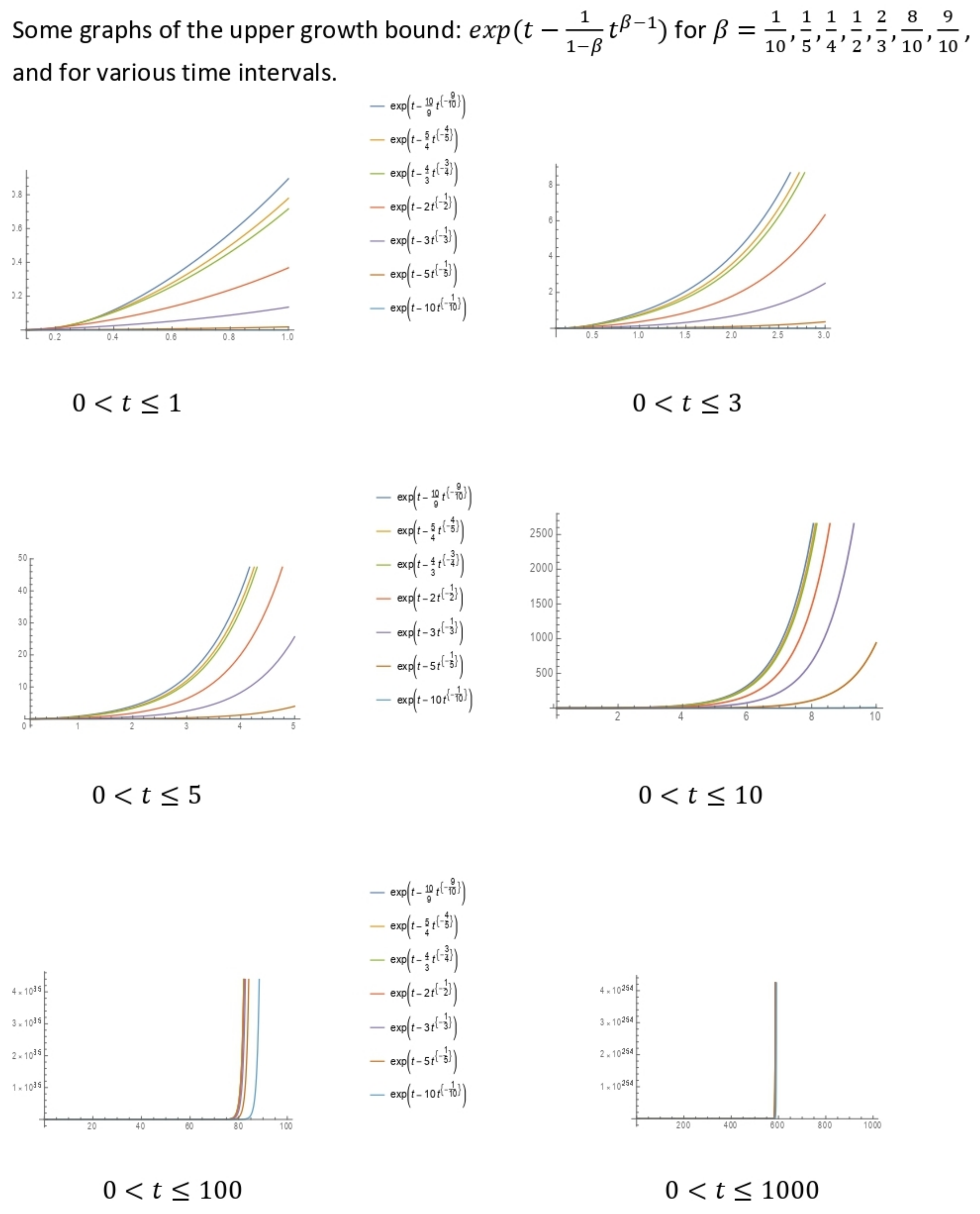
Here, we establish the well-posedness of solution to Equation (3). Now, define

$$\begin{array}{cc}\hfill \mathcal{A}\psi \left(t\right)& ={\psi }_a+\frac{(1-\mu )\upsilon }{\mathbb{AB}\left(\mu \right)}{t}^{\upsilon -1}\varsigma (t,\psi \left(t\right),{}_a^{FFM}{\mathcal{D}}_t^{\mu ,\upsilon }\psi \left(t\right))\hfill \\ \hfill & +\frac{\mu \upsilon }{\mathbb{AB}\left(\mu \right)\Gamma \left(\mu \right)}{\int }_a^t{\tau }^{\upsilon -1}{(t-\tau )}^{\mu -1}\varsigma (\tau ,\psi \left(\tau \right),{}_a^{FFM}{\mathcal{D}}_{\tau }^{\mu ,\upsilon }\psi \left(\tau \right))d\tau ,\hfill \end{array}$$

and obtain the following auxiliary results:

Lemma 3.

Let ψ be a solution satisfying Equation (4) and let Condition 1 be satisfied. Then, it follows that for all $\mu ,\upsilon \in (0,1]$ such that $\mu +\upsilon \ge 1$, we have

$$\parallel \mathcal{A}\psi \parallel \le c_1+c_2\frac{{\mathrm{Lip}}_{\varsigma }}{1-{\mathrm{Lip}}_{\varsigma }}\parallel \psi \parallel ,$$

where $c_1$ and $c_2:=\frac{\upsilon }{\mathbb{AB}\left(\mu \right)}\left[(1-\mu )a^{\upsilon -1}+\frac{\mu \Gamma \left(\upsilon \right)}{\Gamma (\mu +\upsilon )}{T}^{\mu +\upsilon -1}\right]$ are positive constants with $|{\psi }_a|\le c_1$.

Proof. 

By taking absolute value on the operator $\mathcal{A}$, we have

$$\begin{array}{cc}\hfill \left|\mathcal{A}\psi \left(t\right)\right|\le |{\psi }_a|& +\frac{(1-\mu )\upsilon }{\mathbb{AB}\left(\mu \right)}{t}^{\upsilon -1}\left|\varsigma \right(t,\psi \left(t\right),{}_a^{FFM}{\mathcal{D}}_t^{\mu ,\upsilon }\psi \left(t\right)\left)\right|\hfill \\ \hfill & +\frac{\mu \upsilon }{\mathbb{AB}\left(\mu \right)\Gamma \left(\mu \right)}\left|{\int }_a^t{\tau }^{\upsilon -1}{(t-\tau )}^{\mu -1}\varsigma \right(\tau ,\psi \left(\tau \right),{}_a^{FFM}{\mathcal{D}}_{\tau }^{\mu ,\upsilon }\psi \left(\tau \right)\left)d\tau \right|\hfill \\ \hfill \le |{\psi }_a|& +\frac{(1-\mu )\upsilon }{\mathbb{AB}\left(\mu \right)}{t}^{\upsilon -1}\left|\varsigma \right(t,\psi \left(t\right),{}_a^{FFM}{\mathcal{D}}_t^{\mu ,\upsilon }\psi \left(t\right)\left)\right|\hfill \\ \hfill & +\frac{\mu \upsilon }{\mathbb{AB}\left(\mu \right)\Gamma \left(\mu \right)}{\int }_a^t{\tau }^{\upsilon -1}{(t-\tau )}^{\mu -1}\left|\varsigma \right(\tau ,\psi \left(\tau \right){,}_a^{FFM}{\mathcal{D}}_{\tau }^{\mu ,\upsilon }\psi \left(\tau \right)\left)\right|d\tau .\hfill \end{array}$$

Applying Condition 1 and $|{\phi }_a|\le c_1$, to obtain

$$\begin{array}{cc}\hfill \left|\mathcal{A}\psi \left(t\right)\right|\le c_1& +\frac{(1-\mu )\upsilon }{\mathbb{AB}\left(\mu \right)}{t}^{\upsilon -1}{\mathrm{Lip}}_{\varsigma }[\left|\psi \left(t\right)\right|+|{}_a^{FFM}{\mathcal{D}}_t^{\mu ,\upsilon }\psi \left(t\right)\left|\right]\hfill \\ \hfill & +\frac{\mu \upsilon }{\mathbb{AB}\left(\mu \right)\Gamma \left(\mu \right)}{\int }_a^t{\tau }^{\upsilon -1}{(t-\tau )}^{\mu -1}{\mathrm{Lip}}_{\varsigma }[\left|\phi \left(\tau \right)\right|+|{}_a^{FFM}{\mathcal{D}}_{\tau }^{\mu ,\upsilon }\psi \left(\tau \right)\left|\right]d\tau .\hfill \end{array}$$

From Lemma 2, we arrive at

$$\begin{array}{cc}\hfill \left|\mathcal{A}\psi \right(t\left)\right|& \le c_1+\frac{(1-\mu )\upsilon }{\mathbb{AB}\left(\mu \right)}{t}^{\upsilon -1}{\mathrm{Lip}}_{\varsigma }\left[\left|\psi \left(t\right)\right|+\frac{{\mathrm{Lip}}_{\varsigma }}{1-{\mathrm{Lip}}_{\varsigma }}\left|\psi \left(t\right)\right|\right]\hfill \\ \hfill & +\frac{\mu \upsilon }{\mathbb{AB}\left(\mu \right)\Gamma \left(\mu \right)}{\int }_a^t{\tau }^{\upsilon -1}{(t-\tau )}^{\mu -1}{\mathrm{Lip}}_{\varsigma }\left[\left|\psi \left(\tau \right)\right|+\frac{{\mathrm{Lip}}_{\varsigma }}{1-{\mathrm{Lip}}_{\varsigma }}\left|\psi \left(\tau \right)\right|\right]d\tau \hfill \\ \hfill & =c_1+\frac{(1-\mu )\upsilon }{\mathbb{AB}\left(\mu \right)}{t}^{\upsilon -1}\frac{{\mathrm{Lip}}_{\varsigma }}{1-{\mathrm{Lip}}_{\varsigma }}\left|\psi \left(t\right)\right|\hfill \\ \hfill & +\frac{\mu \upsilon }{\mathbb{AB}\left(\mu \right)\Gamma \left(\mu \right)}\frac{{\mathrm{Lip}}_{\varsigma }}{1-{\mathrm{Lip}}_{\varsigma }}{\int }_a^t{\tau }^{\upsilon -1}{(t-\tau )}^{\mu -1}\left|\psi \left(\tau \right)\right|d\tau \hfill \\ \hfill & \le c_1+\frac{(1-\mu )\beta }{\mathbb{AB}\left(\mu \right)}{t}^{\upsilon -1}\frac{{\mathrm{Lip}}_{\varsigma }}{1-{\mathrm{Lip}}_{\varsigma }}\left|\psi \left(t\right)\right|\hfill \\ \hfill & +\frac{\mu \upsilon }{\mathbb{AB}\left(\mu \right)\Gamma \left(\mu \right)}\frac{{\mathrm{Lip}}_{\varsigma }}{1-{\mathrm{Lip}}_{\varsigma }}\parallel \psi \parallel {\int }_a^t{\tau }^{\upsilon -1}{(t-\tau )}^{\mu -1}d\tau .\hfill \end{array}$$

Evaluating the integral above, we have

$$\begin{array}{cc}\hfill \left|\mathcal{A}\psi \right(t\left)\right|& \le c_1+\frac{(1-\mu )\upsilon }{\mathbb{AB}\left(\mu \right)}{t}^{\upsilon -1}\frac{{\mathrm{Lip}}_{\varsigma }}{1-{\mathrm{Lip}}_{\varsigma }}\left|\psi \left(t\right)\right|\hfill \\ \hfill & +\frac{\mu \upsilon }{\mathbb{AB}\left(\mu \right)\Gamma \left(\mu \right)}\frac{{\mathrm{Lip}}_{\varsigma }}{1-{\mathrm{Lip}}_{\varsigma }}\parallel \psi \parallel t^{\mu +\upsilon -1}[B(\mu ,\upsilon )-B_{\frac{a}{t}}(\mu ,\upsilon )]\hfill \\ \hfill & =c_1+\frac{(1-\mu )\upsilon }{\mathbb{AB}\left(\mu \right)}{t}^{\upsilon -1}\frac{{\mathrm{Lip}}_{\varsigma }}{1-{\mathrm{Lip}}_{\varsigma }}\left|\psi \left(t\right)\right|\hfill \\ \hfill & +\frac{\mu \upsilon }{\mathbb{AB}\left(\mu \right)\Gamma \left(\mu \right)}\frac{{\mathrm{Lip}}_{\varsigma }}{1-{\mathrm{Lip}}_{\varsigma }}\parallel \psi \parallel B(\mu ,\upsilon )t^{\mu +\upsilon -1}[1-I_{\frac{a}{t}}(\mu ,\upsilon )]\hfill \\ \hfill & \le c_1+\frac{(1-\mu )\upsilon }{\mathbb{AB}\left(\mu \right)}{t}^{\upsilon -1}\frac{{\mathrm{Lip}}_{\varsigma }}{1-{\mathrm{Lip}}_{\varsigma }}\left|\psi \left(t\right)\right|\hfill \\ \hfill & +\frac{\mu \upsilon }{\mathbb{AB}\left(\mu \right)\Gamma \left(\mu \right)}\frac{{\mathrm{Lip}}_{\varsigma }}{1-{\mathrm{Lip}}_{\varsigma }}\parallel \psi \parallel B(\mu ,\upsilon )t^{\mu +\upsilon -1},\hfill \end{array}$$

(8)

since $1-I_{\frac{a}{t}}(\mu ,\upsilon )\in [0,1].$ We observe that $a^{\upsilon -1}>t^{\upsilon -1}$ since $\upsilon -1<0$. Thus, taking supremum over $t\in [a,T]$ in (8) and recalling that $\mu +\upsilon \ge 1$, we obtain

$$\begin{array}{cc}\hfill \parallel \mathcal{A}\psi \parallel & \le c_1+\frac{(1-\mu )\upsilon }{\mathbb{AB}\left(\mu \right)}{a}^{\upsilon -1}\frac{{\mathrm{Lip}}_{\varsigma }}{1-{\mathrm{Lip}}_{\varsigma }}\parallel \psi \parallel +\frac{\mu \upsilon }{\mathbb{AB}\left(\mu \right)\Gamma \left(\mu \right)}\frac{{\mathrm{Lip}}_{\varsigma }}{1-{\mathrm{Lip}}_{\varsigma }}\parallel \phi \parallel B(\mu ,\upsilon )T^{\mu +\upsilon -1}\hfill \\ \hfill & =c_1+\frac{\upsilon }{\mathbb{AB}\left(\mu \right)}\frac{{\mathrm{Lip}}_{\varsigma }}{1-{\mathrm{Lip}}_{\varsigma }}\left[(1-\mu )a^{\upsilon -1}+\frac{\mu \Gamma \left(\upsilon \right)}{\Gamma (\mu +\upsilon )}{T}^{\mu +\upsilon -1}\right]\parallel \psi \parallel ,\hfill \end{array}$$

and the proof is complete. □

Lemma 4.

Suppose ψ and φ are solutions satisfying Equation (4) and let Condition 1 be satisfied. Then, if it follows that for all $\mu ,\upsilon \in (0,1]$ such that $\mu +\upsilon \ge 1$, we have

$$\parallel \mathcal{A}\psi -\mathcal{A}\phi \parallel \le c_2\parallel \psi -\phi \parallel .$$

Proof. 

The proof is skipped since it follows similar steps as the proof of Lemma 3. □

Next, we state the existence and uniqueness theorem for Equation (3).

Theorem 1.

Let $\alpha +\beta \ge 1$ and suppose Condition 1 is satisfied. Let $c_2>0$, such that $c_2<\frac{1-{\mathrm{Lip}}_{\varsigma }}{{\mathrm{Lip}}_{\varsigma }}$, where $c_2:=\frac{\upsilon }{\mathbb{AB}\left(\mu \right)}\left[(1-\mu )a^{\upsilon -1}+\frac{\mu \Gamma \left(\upsilon \right)}{\Gamma (\mu +\upsilon )}{T}^{\mu +\upsilon -1}\right].$ Then, there exists a unique solution to Equation (3).

Proof. 

We proceed by applying the Banach fixed point theorem. Let $\psi \left(t\right)=\mathcal{A}\psi \left(t\right)$, then using Lemma 3, we have

$$\begin{array}{c}\hfill \parallel \psi \parallel =\parallel \mathcal{A}\psi \parallel \le c_1+c_2\frac{{\mathrm{Lip}}_{\varsigma }}{1-{\mathrm{Lip}}_{\varsigma }}\parallel \psi \parallel .\end{array}$$

Collecting similar terms, we have $\parallel \psi \parallel \left[1-c_2\frac{{\mathrm{Lip}}_{\varsigma }}{1-{\mathrm{Lip}}_{\varsigma }}\right]\le c_1$. This shows that $\parallel \psi \parallel <\infty$ since $c_2<\frac{1-{\mathrm{Lip}}_{\varsigma }}{{\mathrm{Lip}}_{\varsigma }}.$ Furthermore, if $\psi \ne \phi$ are solutions to Equation (3), then from Lemma 4, we have

$$\parallel \psi -\phi \parallel =\parallel \mathcal{A}\psi -\mathcal{A}\phi \parallel \le c_2\frac{{\mathrm{Lip}}_{\varsigma }}{1-{\mathrm{Lip}}_{\varsigma }}\parallel \psi -\phi \parallel .$$

It follows that $\parallel \psi -\phi \parallel \left[1-c_2\frac{{\mathrm{Lip}}_{\varsigma }}{1-{\mathrm{Lip}}_{\varsigma }}\right]\le 0$. Since $1-c_2\frac{{\mathrm{Lip}}_{\varsigma }}{1-{\mathrm{Lip}}_{\varsigma }}>0$, that is, $c_2<\frac{1-{\mathrm{Lip}}_{\varsigma }}{{\mathrm{Lip}}_{\varsigma }},$ then $\parallel \psi -\phi \parallel <0$. This is a contradiction and, therefore, $\parallel \psi -\phi \parallel =0$. □

Exponential Growth

We present an inequality needed in proving the upper growth bound:

Theorem 2

([26]). Given that $f,g,h:I\to {\mathbb{R}}^{+}$ are continuous functions. If $\varphi :I\to {\mathbb{R}}^{+}$ is continuous and

$$\varphi \left(t\right)\le f\left(t\right)+{\int }_{t_0}^t{(t-\tau )}^{\nu -1}g\left(\tau \right)\varphi \left(\tau \right)d\tau +{\int }_{t_0}^t{(t-\tau )}^{\nu -1}h\left(\tau \right){\varphi }^{\gamma }\left(\tau \right)d\tau ,t\in I,$$

with constants $\nu >0$ and $0<\gamma <1$, then the following statements are true.

(i) 

Given that $\nu >\frac{1}{2}$. It follows that

$$\begin{array}{ccc}\hfill \varphi \left(t\right)& \le & [A_1^{1-\gamma }\left(t\right)\hfill \\ & +& (1-\gamma )K_1{\int }_{t_0}^{t}exp\left((\gamma -1)K_1{\int }_{t_0}^s{g}^2\left(\tau \right)d\tau \right)h^2\left(s\right)R_1\left(s\right)ds{]}^{\frac{1}{2(1-\gamma )}}\hfill \\ & \times & exp\left(t+\frac{K_1}{2}{\int }_{t_0}^t{g}^2\left(s\right)ds\right),t\in I,\hfill \end{array}$$

where ${\displaystyle A_1\left(t\right)=\underset{t_0\le s\le t}{max}\left\{2e^{-2s}{f}^2\left(s\right)\right\},}$$K_1=\frac{2\Gamma (2\nu -1)}{4^{\nu -1}},$ and $R_1\left(t\right)=e^{2(\rho -1)t}$.

(ii) 

Given that $\rho \in (0,\frac{1}{2}],\varrho =\frac{1+\nu }{\nu }$ and $p=1+\nu$. Then

$$\begin{array}{ccc}\hfill \varphi \left(t\right)& \le & [A_2^{1-\gamma }\left(t\right)\hfill \\ & +& (1-\gamma )K_2{\int }_{t_0}^{t}exp\left((\gamma -1)K_2{\int }_{t_0}^s{g}^{\varrho }\left(\tau \right)d\tau \right)h^{\varrho }\left(s\right)R_2\left(s\right)ds{]}^{\frac{1}{\varrho (1-\gamma )}}\hfill \\ & \times & exp\left(t+\frac{K_2}{\varrho }{\int }_{t_0}^t{g}^{\varrho }\left(s\right)ds\right),t\in I,\hfill \end{array}$$

where ${\displaystyle A_2\left(t\right)=\underset{t_0\le s\le t}{max}\left\{2^{\varrho -1}{e}^{-s\varrho }{f}^{\varrho }\left(s\right)\right\},K_2=2^{2\varrho -2}{\left(\frac{\Gamma (1-(1-\rho )p}{p^{1-(1-\nu )p}}\right)}^{\frac{\varrho }{p}}}$, and $R_2\left(t\right)=e^{\varrho (\nu -1)t}$.

Theorem 3.

Given that ψ satisfies Equation (4) and the initial function ${\psi }_a$ is bounded above. Suppose Condition 1 is satisfied, then it follows that for all $\mu \in (\frac{1}{2},1]$ and $\upsilon \in [0,1],$ one gets

$$\left|\psi \left(t\right)\right|\le c_{5}exp\left(t-c_6{t}^{\upsilon -1}\right),t\in [a,T],$$

where $c_5={\left(2e^{-2a}{c}_3^2\right)}^{1/2}exp\left(\frac{a^{\upsilon -1}}{1-\upsilon }\right)$ and $c_6={\left(c_4{\mathrm{Lip}}_{\varsigma }\right)}^2\frac{\Gamma (2\mu -1)}{4^{\mu -1}}\frac{1}{1-\upsilon }$ are some positive numbers.

Proof. 

Following from the line of proof of Theorem 3, one obtains

$$\begin{array}{cc}\hfill \left|\psi \right(t\left)\right|& \le c_1+\frac{(1-\mu )\upsilon }{\mathbb{AB}\left(\mu \right)}{t}^{\upsilon -1}\frac{{\mathrm{Lip}}_{\varsigma }}{1-{\mathrm{Lip}}_{\varsigma }}\left|\psi \left(t\right)\right|\hfill \\ \hfill & +\frac{\mu \upsilon }{\mathbb{AB}\left(\mu \right)\Gamma \left(\mu \right)}\frac{{\mathrm{Lip}}_{\varsigma }}{1-{\mathrm{Lip}}_{\varsigma }}{\int }_a^t{\tau }^{\upsilon -1}{(t-\tau )}^{\mu -1}\left|\psi \left(\tau \right)\right|d\tau \hfill \\ \hfill & \le c_1+\frac{(1-\mu )\upsilon }{\mathbb{AB}\left(\mu \right)}{a}^{\upsilon -1}\frac{{\mathrm{Lip}}_{\varsigma }}{1-{\mathrm{Lip}}_{\varsigma }}\left|\psi \left(t\right)\right|\hfill \\ \hfill & +\frac{\mu \upsilon }{\mathbb{AB}\left(\mu \right)\Gamma \left(\mu \right)}\frac{{\mathrm{Lip}}_{\varsigma }}{1-{\mathrm{Lip}}_{\varsigma }}{\int }_a^t{\tau }^{\upsilon -1}{(t-\tau )}^{\mu -1}\left|\psi \left(\tau \right)\right|d\tau .\hfill \end{array}$$

(9)

Let $\mathrm{Y}\left(t\right):=\left|\psi \right(t\left)\right|$ and ${\tilde{c}}_2:=1-\frac{{\mathrm{Lip}}_{\varsigma }}{1-{\mathrm{Lip}}_{\varsigma }}\frac{a^{\upsilon -1}(1-\mu )\upsilon }{\mathbb{AB}\left(\mu \right)}>0$. Thus, for ${\mathrm{Lip}}_{\varsigma }<$$\frac{\mathbb{AB}\left(\mu \right)}{\mathbb{AB}\left(\mu \right)+\upsilon (1-\mu )a^{\upsilon -1}}$, it follows from (9) that

$${\tilde{c}}_2\mathrm{Y}\left(t\right)\le c_1+\frac{\mu \upsilon }{\mathbb{AB}\left(\mu \right)\Gamma \left(\mu \right)}\frac{{\mathrm{Lip}}_{\varsigma }}{1-{\mathrm{Lip}}_{\varsigma }}{\int }_a^t{\tau }^{\upsilon -1}{(t-\tau )}^{\mu -1}\mathrm{Y}\left(\tau \right)d\tau .$$

Now, dividing by ${\tilde{c}}_2=\frac{\mathbb{AB}\left(\mu \right)-{\mathrm{Lip}}_{\varsigma }\left[\mathbb{AB}\left(\mu \right)+\upsilon (1-\mu )a^{\upsilon -1}\right]}{(1-{\mathrm{Lip}}_{\varsigma })\mathbb{AB}\left(\mu \right)}$, to get

$$\mathrm{Y}\left(t\right)\le c_3+c_4{\mathrm{Lip}}_{\varsigma }{\int }_a^t{\tau }^{\upsilon -1}{(t-\tau )}^{\mu -1}\mathrm{Y}\left(\tau \right)d\tau ,$$

with $c_3:=\frac{c_1}{{\tilde{c}}_2}$ and $c_4:=\frac{\mu \upsilon }{\Gamma \left(\mu \right)\left(\mathbb{AB}\left(\mu \right)-{\mathrm{Lip}}_{\varsigma }\left[\mathbb{AB}\left(\mu \right)+(1-\mu )\upsilon a^{\upsilon -1}\right]\right)}$. Next, using Theorem 2 (i) with $h\left(\tau \right)=0,g\left(\tau \right)=c_4{\mathrm{Lip}}_{\varsigma }{\tau }^{\upsilon -1}$ and $\nu =\mu >\frac{1}{2}$, to obtain

$$\begin{array}{ccc}\hfill \mathrm{Y}\left(t\right)& \le & A_1^{1/2}\left(t\right)exp\left(t+\frac{K_1}{2}{\left(c_4{\mathrm{Lip}}_{\varsigma }\right)}^2{\int }_a^t{\tau }^{2\upsilon -2}d\tau \right)\hfill \\ & =& A_1^{1/2}\left(t\right)exp\left(t+{\left(c_4{\mathrm{Lip}}_{\varsigma }\right)}^2\frac{\Gamma (2\mu -1)}{4^{\mu -1}}\frac{t^{\upsilon -1}-a^{\upsilon -1}}{\upsilon -1}\right)\hfill \\ & =& {\left(2e^{-2a}{c}_3^2\right)}^{1/2}exp\left(\frac{a^{\upsilon -1}}{1-\upsilon }\right)exp\left(t-{\left(c_4{\mathrm{Lip}}_{\varsigma }\right)}^2\frac{\Gamma (2\mu -1)}{4^{\mu -1}}\frac{t^{\upsilon -1}}{1-\upsilon }\right),\hfill \end{array}$$

where $K_1=\frac{2\Gamma (2\mu -1)}{4^{\mu -1}}$ and ${\displaystyle A_1\left(t\right)=\underset{a\le s\le t}{max}\left\{2e^{-2s}{c}_3^2\right\}=2e^{-2a}{c}_3^2}$, since $e^{-2t}$ is decreasing. □

3.2. Asymptotic Property of the Solution

Here, we show the long term (limiting) property of our solution. The corollary indicates that the rate of energy growth of the solution is finite when time becomes large.

Corollary 1.

Under the hypotheses of Theorem 3 and for all $0<\beta <1$, we have

$$\underset{t\to \infty }{lim\; sup}\frac{log\left|\phi \right(t\left)\right|}{t}\le 1.$$

Proof. 

We obtained from Thereom 3 that

$$\left|\psi \left(t\right)\right|\le c_{5}exp\left(t-c_6{t}^{\upsilon -1}\right),t\in [a,T].$$

If we take log of both sides of the above equation, it will yield

$$log\left|\psi \left(t\right)\right|\le log\left(c_5\right)+t-c_6{t}^{\upsilon -1}.$$

Next, divide through by t to obtain

$$\frac{log\left|\psi \right(t\left)\right|}{t}\le \frac{log\left(c_5\right)}{t}+1-c_6\frac{t^{\upsilon -1}}{t}=\frac{log\left(c_5\right)}{t}+1-\frac{c_6}{t^{2-\upsilon }}.$$

Since $0<\upsilon <1$, it follows that $2-\upsilon \ge 1$. Now, take limit supremum over t in both sides to get

$$\underset{t\to \infty }{lim\; sup}\frac{log\left|\psi \right(t\left)\right|}{t}\le \underset{t\to \infty }{lim\; sup}\frac{log\left(c_5\right)}{t}+1-\underset{t\to \infty }{lim\; sup}\frac{c_6}{t^{2-\upsilon }}=1.$$

□

4. Examples

Now, we give examples to illustrate the result in Theorem 3. The following are some plots (graphs) for the upper bound growth of our energy solution $\left|\psi \left(t\right)\right|\le exp(t-\frac{1}{1-\upsilon }{t}^{\upsilon -1}),t\in [a,T]$. For convenience, we set $c_5=1$ and choose $\mu \in (\frac{1}{2},1]$, such that $c_6=\frac{1}{1-\upsilon }$ with $c_4=1,{\mathrm{Lip}}_{\varsigma }=1$. We plotted graphs of the growth bound for $\upsilon =\frac{1}{10},\frac{1}{5},\frac{1}{4},\frac{1}{2},\frac{2}{3},\frac{8}{10},\frac{9}{10}$, and for various time intervals. It is observed that as closer the parameter $\upsilon$ is to zero, the faster the rate of growth is to the bound. However, as time grows large, the growth rate is at most at $t=600$ irrespective of the values of $\upsilon$, as shown in the Figure 1 below.

5. Conclusions

Fractional order derivatives are used to represent memory formalism in modeling phenomena or processes in porous media in order to diminish the size of the pores and the permeability of the porous matrix [27]. Hence, implicit fractal–fractional differential equations are very important because they model many technical processes and systems in porous environment exhibiting long time memory property. In this paper, we estimated the higher growth bound of our solution and it is shown that the solution exhibits an exponential growth in t at a specific rate. Furthermore, the result shows a long time behaviour of the mild solution. Banach fixed point theorem was applied to prove the well-posedness of mild solution to the class of implicit time–fractal–fractional differential equation with Mittag–Leffler law. For future work, one can investigate the lower growth estimate of the solution, the stability of the solution, and the continuous dependence on the initial condition, as shown in [20].

References

1. Atangana, A. Fractal–fractional differentiation and integration: Connecting fractal calculus and fractional calculus to predict complex system. Chaos Solit. Fract. 2017, 102, 396–406. [Google Scholar] [CrossRef]
2. Atangana, A.; Akgu¨l, A.; Owolabi, K.M. Analysis of Frac-tal–fractional differential equations. Alex. Eng. J. 2020, 59, 1117–1134. [Google Scholar] [CrossRef]
3. Araz, S.I. Numerical analysis of a new Volterra integro-differential equation involving fractal–fractional operators. Chaos Solit. Fract. 2020, 130, 109396. [Google Scholar] [CrossRef]
4. Owolabi, K.M.; Atangana, A.; Akgu¨l, A. Modelling and Analysis of Fractal-fractional partial differential equations: Application to reaction-diffusion model. Alex. Eng. J. 2020, 59, 2477–2490. [Google Scholar] [CrossRef]
5. He, J.-H. Fractal calculus and its geometrical explanation. Results Phys. 2018, 10, 272–276. [Google Scholar] [CrossRef]
6. Hosseininia, M.; Heydari, M.H.; Avazzadeh, Z. The Numerical Treatment of Non-linear Fractal–fractional 2D EMDEN-FOWLER equation utilizing 2D Chelyshkov polynomials. Fractals 2020, 28, 2040042. [Google Scholar] [CrossRef]
7. Gómez-Aguilar, J.F.; Atangana, A. New chaotic attractors: Applications of fractal-fractional differentiation and integration. Math. Methods Appl. Sci. 2020, 44, 3036–3065. [Google Scholar] [CrossRef]
8. Saad, K.M.; Alqhtani, M.; Gómez-Aguilar, J.F. Fractal-fractional study of the hepatitis C virus infection model. Results Phys. 2020, 19, 103555. [Google Scholar] [CrossRef]
9. Zuniga-Aguilar, C.J.; Gómez-Aguilar, J.F.; Romero-Ugalde, H.M.; Ja-hanshahi, H.; Alsaadi, F.E. Fractal-fractional neuro-adaptive method for system identification. Eng. Comput. 2020, 240, 1–24. [Google Scholar] [CrossRef]
10. Abro, K.A.; Atangana, A.; Gómez-Aguilar, J.F. Ferromagnetic chaos in thermal convection of fluid through fractal-fractional differentiation. J. Therm. Anal. Calorim. 2022, 147, 8461–84733. [Google Scholar] [CrossRef]
11. Nane, E.; Nwaeze, E.R.; Omaba, M.E. Asymptotic behavior and non-existence of global solution to a class of conformable time-fractional stochastic differential equation. Stat. Probab. Lett. 2020, 163, 108792. [Google Scholar] [CrossRef] [Green Version]
12. Omaba, M.E. On Space-Fractional Heat Equation with Non-homogeneous Fractional Time Poisson Process. Progr. Fract. Differ. Appl. 2020, 6, 67–79. [Google Scholar]
13. Omaba, M.E.; Nwaeze, E.R. Moment Bound of Solution to a Class of Conformable Time-Fractional Stochastic Equation. Fractal Fract. 2019, 3, 18. [Google Scholar] [CrossRef] [Green Version]
14. Asma; Gómez-Aguilar, J.F.; ur Rahman, G.; Javed, M. Stability for fractional order implicit ψ-Hilfer differential equations. Math. Methods Appl. Sci. 2021, 45, 2701–2712. [Google Scholar] [CrossRef]
15. Benchohra, M.; Lazreg, J.E. Existence results for nonlinear implicit fractional dif-ferential equations. Surv. Math. Its Appl. 2014, 9, 79–92. [Google Scholar]
16. Borisut, P.; Bantaojai, T. Implicit fractional differential equations with nonlocal frac-tional integral conditions. Thai J. Math. 2021, 19, 993–1003. [Google Scholar]
17. Shabbir, A.S.; Shah, K.; Abdeljawad, T. Stability analysis for a class of implicit frac-tional differential equations involving Atangana–Baleanu fractional derivative. Adv. Differ. Equ. 2021, 2021, 395. [Google Scholar] [CrossRef]
18. Benchohra, M.; Souid, M.S. Integrable solutions for implicit fractional order dif-ferential equations. Arch. Math. 2015, 51, 67–76. [Google Scholar]
19. Benchohra, M.; Bouriaha, S. Existence and stability results for nonlinear boundary value problem for implicit differential equations of fractional order. Moroc. J. Pure Appl. Anal. 2017, 1, 22–37. [Google Scholar] [CrossRef] [Green Version]
20. Kucche, K.D.; Nieto, J.J.; Venktesh, V. Theory of nonlinear implicit fractional differ-ential equations. Diff. Equ. Dyn. Syst. 2016, 38, 1–17. [Google Scholar]
21. Nieto, J.J.; Ouahab, A.; Venktesh, V. Implicit fractional differential equations via Liou-ville–Caputo derivative. Mathematics 2015, 3, 398–411. [Google Scholar] [CrossRef]
22. Atangana, A.; Baleanu, D. New fractional derivatives with nonlocal and nonsingular kernel: Theory and application to heat transfer model. Therm. Sci. 2016, 20, 763–769. [Google Scholar] [CrossRef] [Green Version]
23. Srivastava, H.M.; Choi, J. Zeta and q-Zeta Functions and Associated Series and Inte-Grals; Elsevier: Amsterdam, The Netherlands, 2012; pp. 1–140. [Google Scholar]
24. Helton, J.W.; Klep, I.; Mccullough, S.; Schweighofer, M. Dilations, linear matrix ine-qualities, the matrix cube problem and beta distribution. Memiors Am. Math. Soc. 2019, 257, 1232. [Google Scholar]
25. Aono, Y.; Nguyen, P.Q.; Seito, T.; Shiketa, J. Lower Bounds on Lattice Enumeration with Extreme Pruning. In Proceedings of the 38th Annual International Cryptology Conference, IACR, Santa-Barbara, CA, USA, 19–23 August 2018. [Google Scholar] [CrossRef] [Green Version]
26. Shao, J.; Meng, F. Gronwall-Bellman Type Inequalities and Their Applications to Frac-tional Differential equations. Abstr. Appl. Anal. 2013, 2013, 217641. [Google Scholar] [CrossRef] [Green Version]
27. Di Giuseppe, E.; Moroni, M.; Caputo, M. Flux in porous Media with Memory: Models and Experiment. Transp. Porous. Med. 2010, 83, 479–500. [Google Scholar] [CrossRef]
Figure 1. Graphical illustration of the growth bounds.
Axioms 11 00348 g001
Publisher’s Note: MDPI stays neutral with regard to jurisdictional claims in published maps and institutional affiliations.