Abstract
This paper addresses a modified epidemic model with saturated incidence and incomplete treatment. The existence of all equilibrium points is analyzed. A reproduction number is determined. Next, it is found that the non-endemic point is stable in case , but unstable in case . The special conditions to analyze the local and global stability of the non-endemic and endemic points are investigated. Globally, the sensitivity analysis of the system is studied by combining the Latin Hypercube Sampling and Partial Rating Correlation Coefficients methods. By using the Pontryagins maximum principle, the optimal control problem is studied. Various numerical results are given to support our analysis.
1. Introduction
Population dynamics in the spread of infectious diseases can be studied through a mathematical model. Mathematically, in epidemiological modeling, there is one deterministic model, namely, the model. A model is generalized of several epidemic models (e.g., , , and ) involving the relationships of several sub-classes in the human population among the susceptible S, latent/exposed E, infectious I, and recovered/healed R, for understanding the behavioral contagion for a disease. Related to the model, several researchers have used it to solve their problems, including analyzing disease behavior. For example: COVID-19 (see [1,2,3]), Malaria (see [4]), Hand Foot Mouth Disease (see [5]), Measles (see [6]), Influenza A (H1N1) (see [7]), Zika Fever (see [8,9]), as well as Tuberculosis (TB) (see [10]). It is not just limited to the spread of disease in the human population; the model has been implemented to study virus mutation of wireless sensor networks [11] and also the propagation of computer viruses [12].
Because of the limited resources available to eradicate a disease, treatment is not only carried out in the hospitals. However, treatment also can be performed at home, providing an adequate service was established [13] for effective home treatment based on the behavior of the disease to accelerate recovery and prevent the hospitalization of patients. This process would have significant impacts on the patients and also the health system [14]. Implementing the proposed outpatient treatment during the mild phase of the disease reduced the incidence of subsequent hospitalization and related costs [15]. Through the mathematical models, this aspect is considered in work regarding a specific disease by some researchers (see [16,17]). In conditions where the proportion of infections increases, hospitalization policies may be needed to deal with the number of infection cases [18].
On the other hand, researchers have analyzed the impact of incomplete treatment on disease transmission, and when incomplete treatment occurs, an infectious individual can be fitted into latent again [19]. Relapse may occur, where a recovered human can be fitted back into latent due to the reactivation of the infectious agents. For example, Herpes [20] and Tuberculosis [21,22,23,24,25] are of this type. This relates to an infected individual that may disappear after treatment, but infectious agents may remain in the person’s body after being treated. Thus the person being treated can possibly still be a carrier of the disease and return to the latent/exposed class [19,22]. It shows that incomplete treatment for patients may lead to a complicated situation.
From the various studies conducted above, researchers have used a bilinear form for the incidence rate. However, in reality, related to epidemic cases, the form of the bilinear incidence rate is only effective in the early stages. There are many studies that have discussed nonlinear incidence rates for epidemic problems; this includes models with the saturated infection rate [26,27,28,29,30,31,32,33]. Occasionally, the saturated function, also named Holling type-II function [34], has been used by some researchers for analyzing the population dynamics because of a specific disease model (see [35,36,37,38,39,40,41]).
Here, we propose an epidemic model for disease outbreaks with a saturated incidence rate and incomplete treatment. Our model is extended from the epidemic model by Huo and Zou in [16]. The novelty in our work is the consideration of the saturated infection of humans who come into contact with infectious humans who are undergoing treatment at home and treatment in hospital. This work is clearly different from previous studies that have also used saturated infection, see [26,27,28,29,30,31,32,33,34,35,36,37,38,39,40,41]. We also consider an aspect of incomplete treatment, which makes our work relatively new for the epidemic model. Despite the lack of data, this does not detract from the essence of analyzing and simulating the model. The paper is organized as follows. In Section 2 we construct our model. We determine the special conditions to analyze the existence and the local and global stability of equilibrium in Section 3. In Section 4, we perform some numerical results to confirm our analysis, including the sensitivity analysis and the optimal control strategy. Finally, we give some remarks to conclude our work in Section 5.
2. Model Formulation
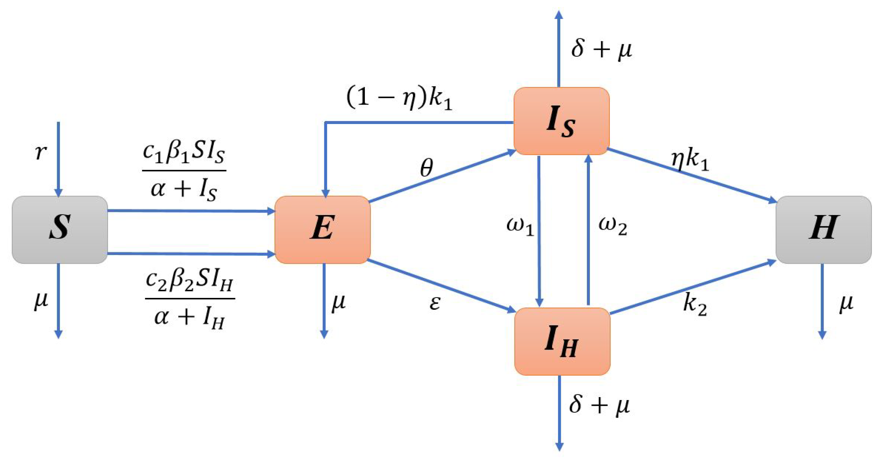
We constructed an epidemic model of disease outbreak by considering saturated infection and incomplete treatment. The total population is , which is classified into five classes, namely, susceptible humans (S), latent/exposed humans (E), infectious humans treated at home (), infectious humans treated in the hospital (), and healed/recovered humans (H), where:
The assumptions used in the formation of mathematical models for disease spread are whether the individual infected will receive hospitalization or outpatient treatment. Next, the individuals with incomplete treatment may become reinfected, thus reenter the latent class because of incomplete treatment experienced by patients. Hence, that individual could be infection and reenter to latent again. Furthermore, the following assumptions are taken in deriving the model (1):
Assumption 1.
There are constant recruitments to the system for class S, which are denoted by . and the natural mortality for each class in the population has a constant rate of .
Assumption 2.
The first type of contact with is the transfer from S to E by contact; according to the saturated incidence rate with maximum contact rate , the probability of transfer of the disease is given by and the intervention level (half saturated constant). While the second type of contact with is the transfer from S to E by contact, according to the saturated incidence rate with a maximum contact rate , and a probability of transfer of the disease given by .
Assumption 3.
The humans with symptoms will be transferred from E to with a rate and E to denoted by . Next, is the rate of progression from to , while , conversely, is to .
Assumption 4.
Humans leave class at a rate of , a fraction of which enter the recovered class due to efficient treatment and reenter class E due to incomplete treatment. The parameter reflects the part of efficient treatment. While shows the successful treatment for humans in class .
Assumption 5.
Regarding the mortality caused by the same disease for both and , respectively, there is the mortality rate denoted by .
Next, the scheme of disease transmission is illustrated in Figure 1; for the description of notations see Table 1.
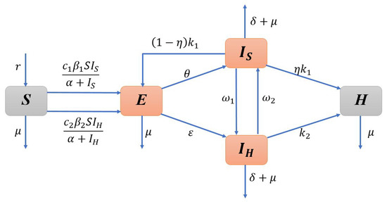
Figure 1.
Diagram of Population Interations.

Table 1.
Parameters Description.
Therefore, based on the interaction diagram in Figure 1, the mathematic model of disease transmission can be constructed:
3. Mathematical Analysis
3.1. Positivity and Boundedness of Solutions
Theorem 1.
Proof.
Refer to positive proving by Huo and Zou in [16], as well as Omame and Okuonghae in [42]. If , , , , , then from the first equation in (1) viz:
It can be re-written as:
Therefore,
Hence,
Therefore,
Consistently, we can apply the similar method to prove that , , , . Hence, the solution in system (1) is positive for all time . □
Theorem 2.
The solution of system (1) is bounded for all
3.2. Non-Endemic Equilibrium Point
By setting the derivatives of each equation in system (1) to zero, i.e., , , , , , and next substituting , , we get the non-endemic point as:
3.3. Basic Reproduction Number
The Basic Reproduction Number () is the average number of newly generated infected humans by a single positively patient. Next, from system (1), we get:
Next,
where
Next, the eigenvalues of are:
The spectral radius of matrix is , where:
For , this means there is no incomplete treatment. Even farther, if we replace with , then
Obviously, thus the high level of incomplete treatment led to increases. This means that the spread of the disease within the population may increase due to incomplete treatment.
3.4. Endemic Equilibrium Points
To determine the endemic point, we consistently set all derivatives in all equations in (1) to zero. Next, from the calculations for these all equations, except the third equation, we get:
3.5. Local Stability of Equilibrium Points
To investigate the local stability around each equilibrium point, we determined the Jacobian matrix and analyzed their eigenvalues for all points, which the Jacobian matrix for system (1) is
Theorem 3.
A non-endemic point of the system (1) is locally asymptotically stable for , and it is unstable for .
Proof.
At , we get that the Jacobian matrix for system (1), which has eigenvalues .
Next, we have a characteristic polynomial
where:
From the polynomial , the real part of will be negative if , , and . Since , , and are fulfilled, for every parameter in system (1). Thus, if and Routh-Hurwitz’s criteria holds, then the non-endemic point is locally asymptotically stable. □
Theorem 4.
An endemic point of the system (1) is locally asymptotically stable whenever it is exists.
Proof.
At , the Jacobian matrix for the system (1) has eigenvalues and . Next, we have a characteristic polynomial
where:
From the polynomial , the real part of will be negative if , , and . Since and are fulfilled, for every parameter in system (1). Thus, whenever exists and the Routh-Hurwitz’s criteria holds, it leads to endemic point () being locally asymptotically stable. □
3.6. Global Stability of Equilibrium Points
Theorem 5.
A non-endemic point of the system (1) is globally asymptotically stable for and it is unstable for .
Proof.
To prove the global stability of , we refer to work by Ullah et al. in [21] as well as Huo and Zou in [16], and define the Lyapunov function
where
The derivative of with respect to t is
Based on Theorem 2, if the solution of system (1) is bounded by as then the non-endemic point is bounded by . Next, choosing we get:
Clearly, if , then . It led to the non-endemic point being globally asymptotically stable. This completes the proof. □
Theorem 6.
Since an endemic point of the system (1) exists, it is globally asymptotically stable.
Proof.
Refering to the various studies in [43,44,45], we define the Lyapunov function
where . Furthermore, the derivative of with respect to t is
By setting , next, , , , , and are used to compute as follows:
- For , we get
- For , we get
- For , we get
- For , we get
- For , we get
Now, we have
where
Next, applying the relationship from the geometric means and arithmetic means, we affirm that . It holds only at point . Thus, the endemic point is globally asymptotically stable. □
3.7. Control Optimal Problem
In order to control the transmission of the disease, our goal was to reduce the amount of the two infected populations through both home treatment and hospital treatment. How we can reduce the infected population is through educational effort, both directly and indirectly. Health workers can educate about the times to consume medicine that better benefits the patients, follow up on the patient’s health activities, etc. To reduce the number of infected people and optimize the educational effort to control cost, we remodeled the dynamic model, adding a parameter for control . Then, we obtain:
We determine the educational effort with the objective function as follows:
Parameters A, B, and C are the weight of the infected population and educational effort in the performance index that satisfies . We solve the optimal control for model with the Pontryagin Maximum Principle. The control v with the variable state and the constraint on (7).
The system ought to satisfy the conditions: and , , , , , where is the control upper limit. Note that the control v represents the percentage of the control. This parameter describes the maximum effort related to control management, and then it is stated as . We build the function of Hamiltonian as , which is equal to
where , , , , and are the Lagrange multipliers of the optimization problem or known as the co-state variables in optimal control theory. Next, related to the necessary condition for the optimal control problems, noted that it should satisfy the Pontryagin Maximum Principle as follows:
- State equations for this model rewriting with the condition, , , ,
- Co-state equation
- Stationer condition , with , then we getbecause satisfies the minimization problem of the optimal control with as the optimal control of system.
4. Numerical Simulation
In this section, we present a numerical simulation to show the behavior of an epidemic model with a saturation incidence rate and incomplete treatment. It should support our analysis in the earlier section. For numerical examples, we use some hypothetical values of the parameters in Table 2. The results are summarized in the figures that follow.
Table 2.
Values of the parameter occurring in the model.
4.1. Case for
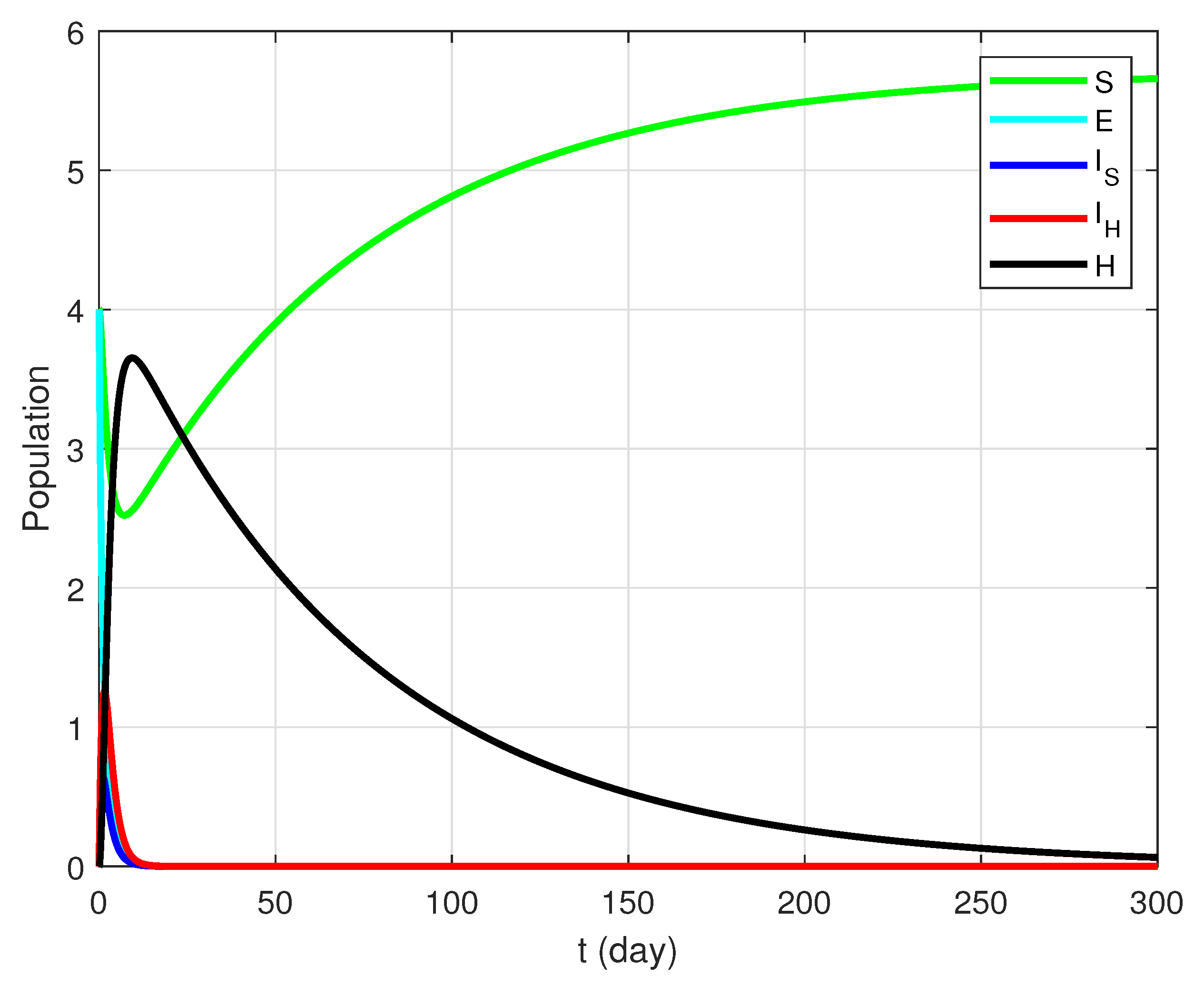
In this subsection, we provide an example and numerical results to support our theoretical results. We set and , as well as consistently using the parameter values in Table 2. By calculating, model (1) has the endemic point (2.9591, 0.0246, 0.0120, 0.0323, 2.0518). Based on Theorem 4 and also Theorem 6, point is asymptotically stable because and all of the eigenvalues are negative (see Appendix A). The behavior of this case is depicted in Figure 2.
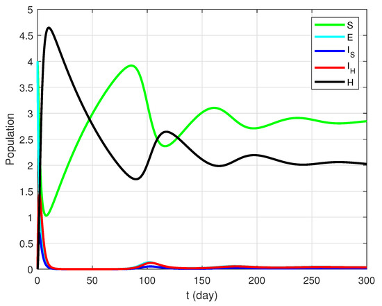
Figure 2.
The dynamics of all classes when we set the parameters and . The endemic point is asymptotically stable.
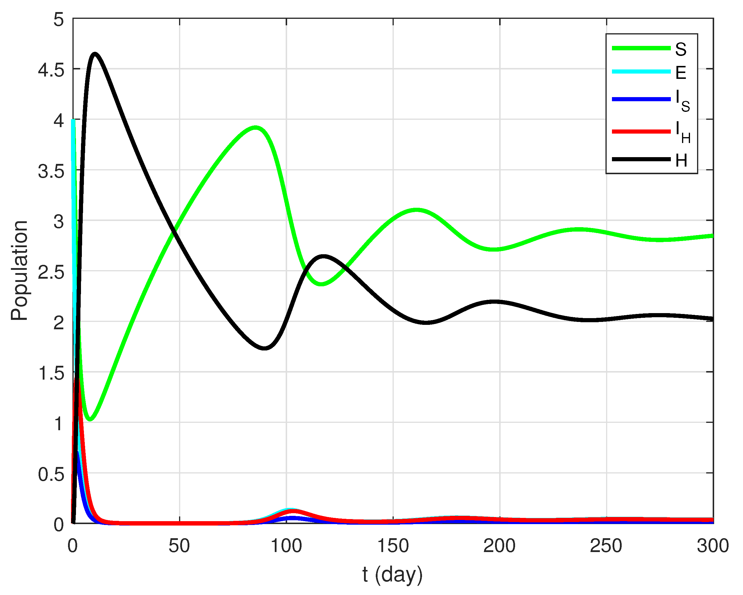
4.2. Case
Next, consistently, the values of the parameter model in Table 2 are used, except and . The initial conditions are the same as those in the above case. From the calculation results, model (1) has the non-endemic point . In addition, from Theorem 3 and also Theorem 5, the non-endemic point is asymptotically stable because and all of the eigenvalues are negative (see Appendix B). The graph for this case is presented in Figure 3.

Figure 3.
The dynamics of all classes when we set the parameters and . The non-endemic point is asymptotically stable.
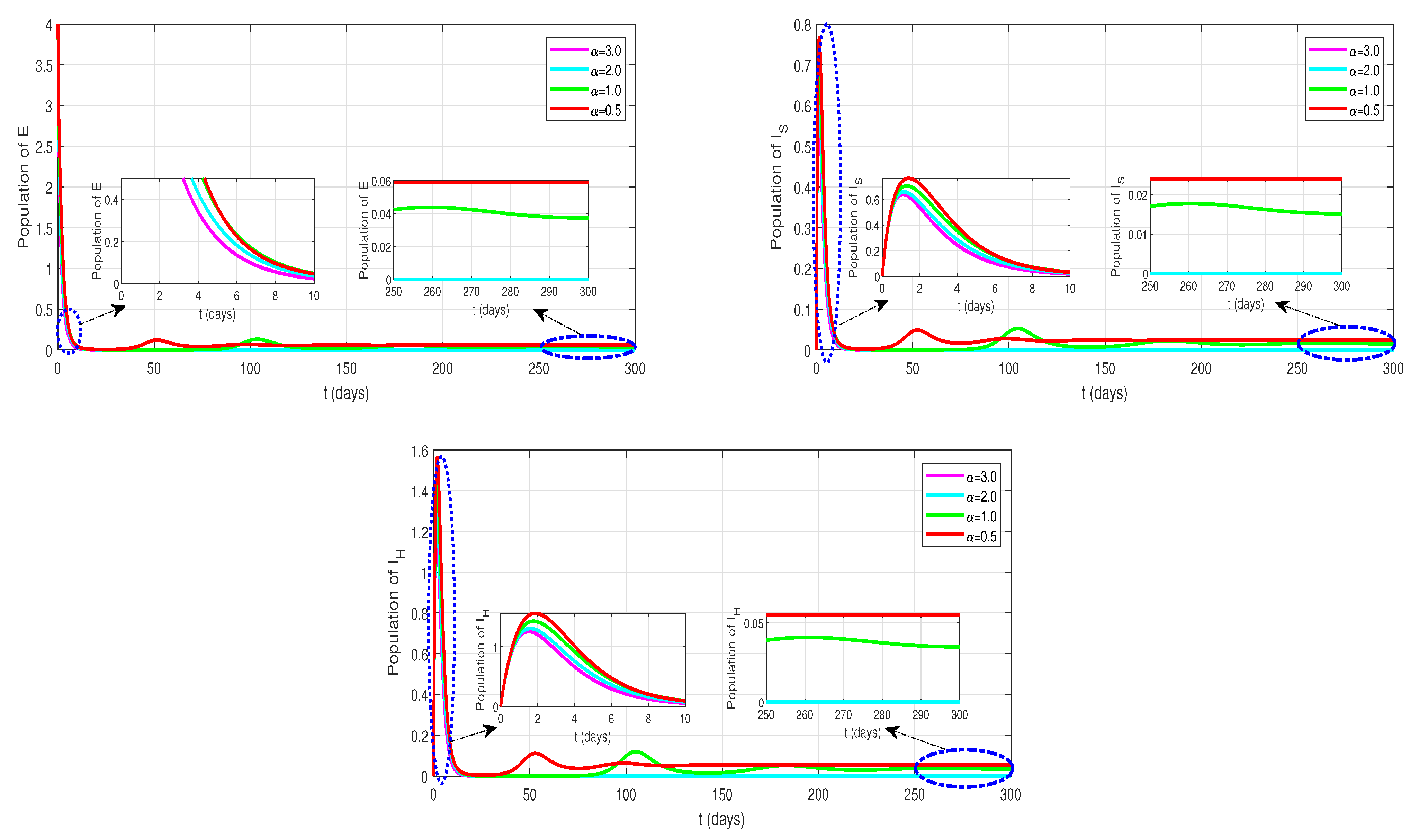
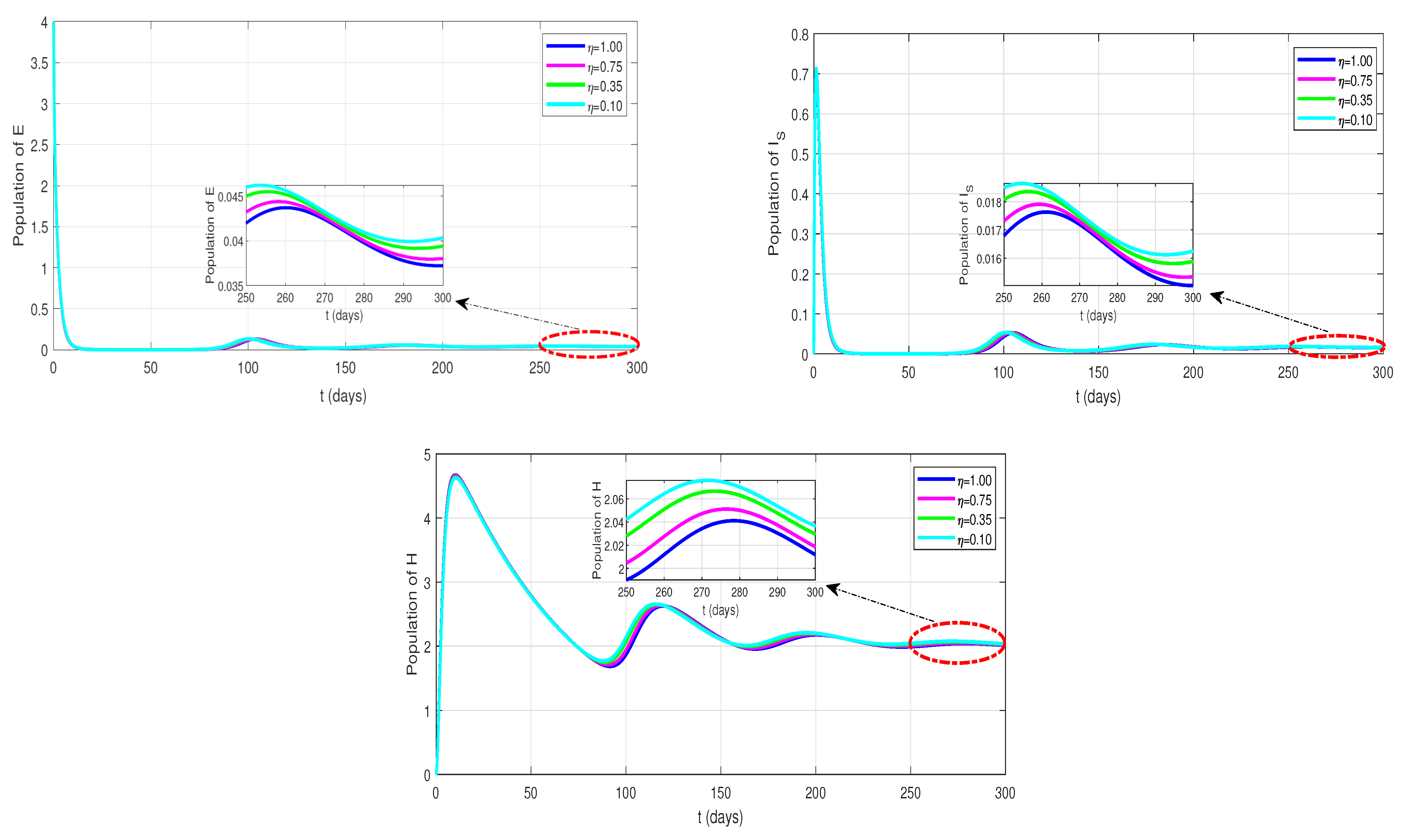
4.3. Effect of Parameters and on
In this sub-section, we simulate the sensitivity analysis for and , related to the saturated incidence rate and incomplete treatment. The parameter values in Table 2 and the same initial values as the previous cases are used to simulate.
- (1)
- For the study the effect of saturated incidence rate, we choose the various of , where and . The details of each change due to the value-change for the rate of saturated incidence () on the , and classes can be seen in Figure 4. Significantly, the value-changes of have an impact on the humans of E, and . Thus, the changes in the parameter value of the saturated incidence really influented the numbers of exposed (E), infected humans with home treated (), and infected humans with hospital treated ().
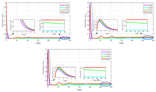 Figure 4. Dynamics of E, , and for and showing the impact of saturated incidence rate.
 - (2)
- Next, to study the effect of the rate of incomplete treatment, we choose the various of , where and . The value-changes of incomplete treatment () affect the population of each class: E, , and H are illustrated in Figure 5. When the value of the incomplete treatment is increased, the impact has reduced the number of exposed (E), and infected humans with home treated (). Meanwhile, the number of humans in the healed class (H) increases. Thus, the humans of , and classes are relatively changed for every .
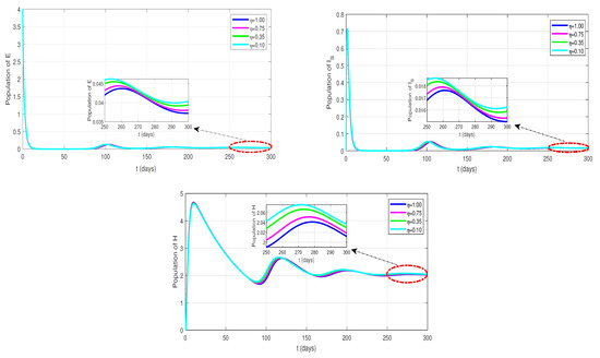 Figure 5. Dynamics of E, , and H for and showing the effect of incomplete treatment at home.
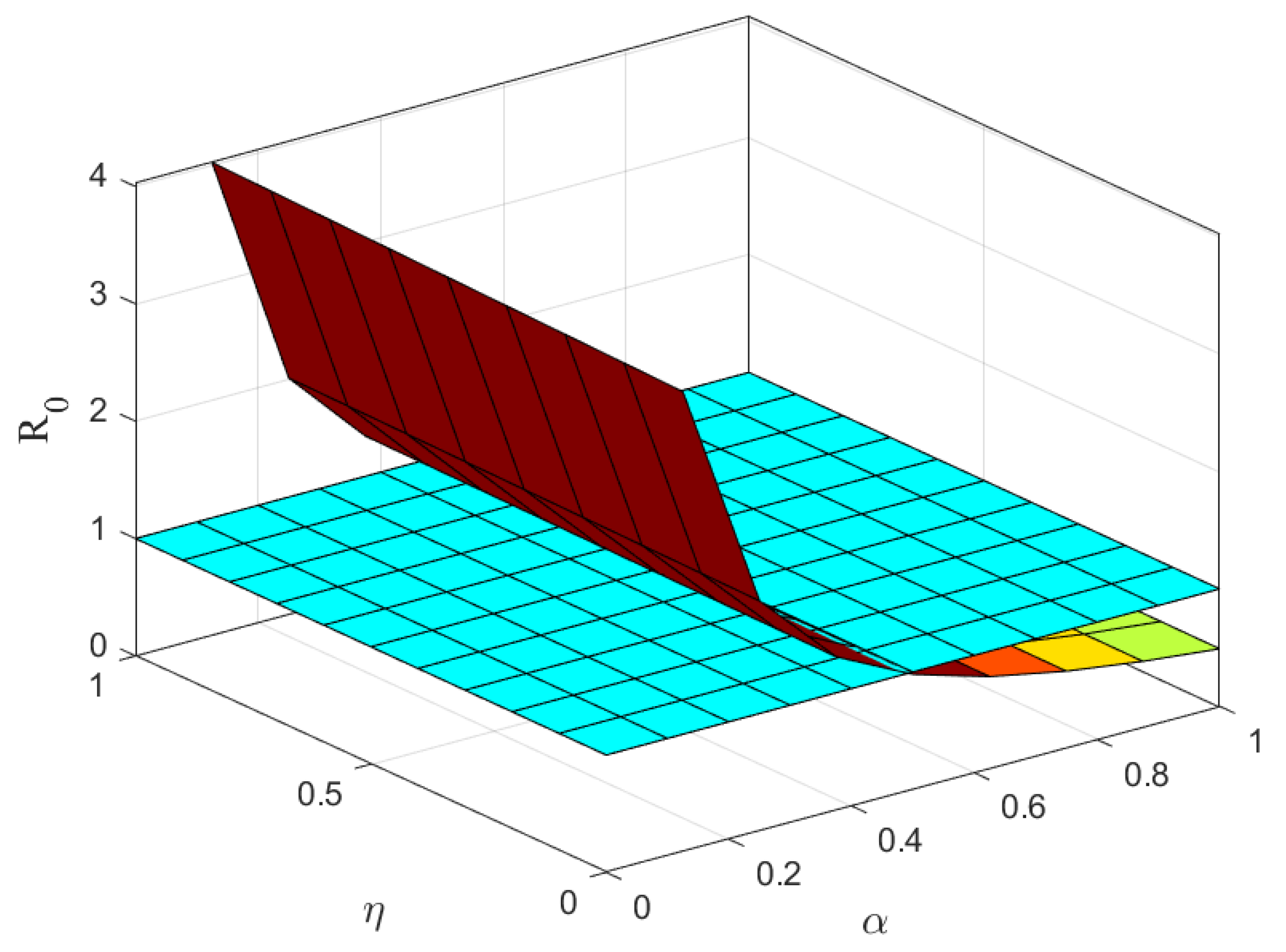
Furthermore, in Figure 6 a relationship among , , and has been shown. If the values of and increase measurably, then the number of decreases sharply. This illustrates that increasing the level of treatment and the rate of saturated incidence has an immediate impact on reducing the number of infections in humans.

Figure 6.
The relationship among , , and .
4.4. Partial Rank Correlation Coefficient
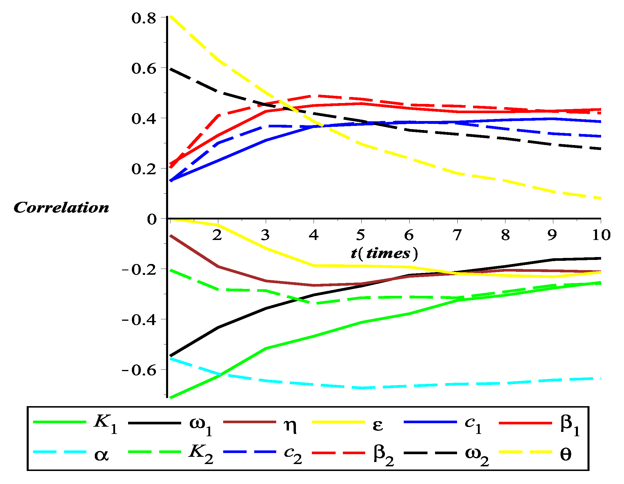
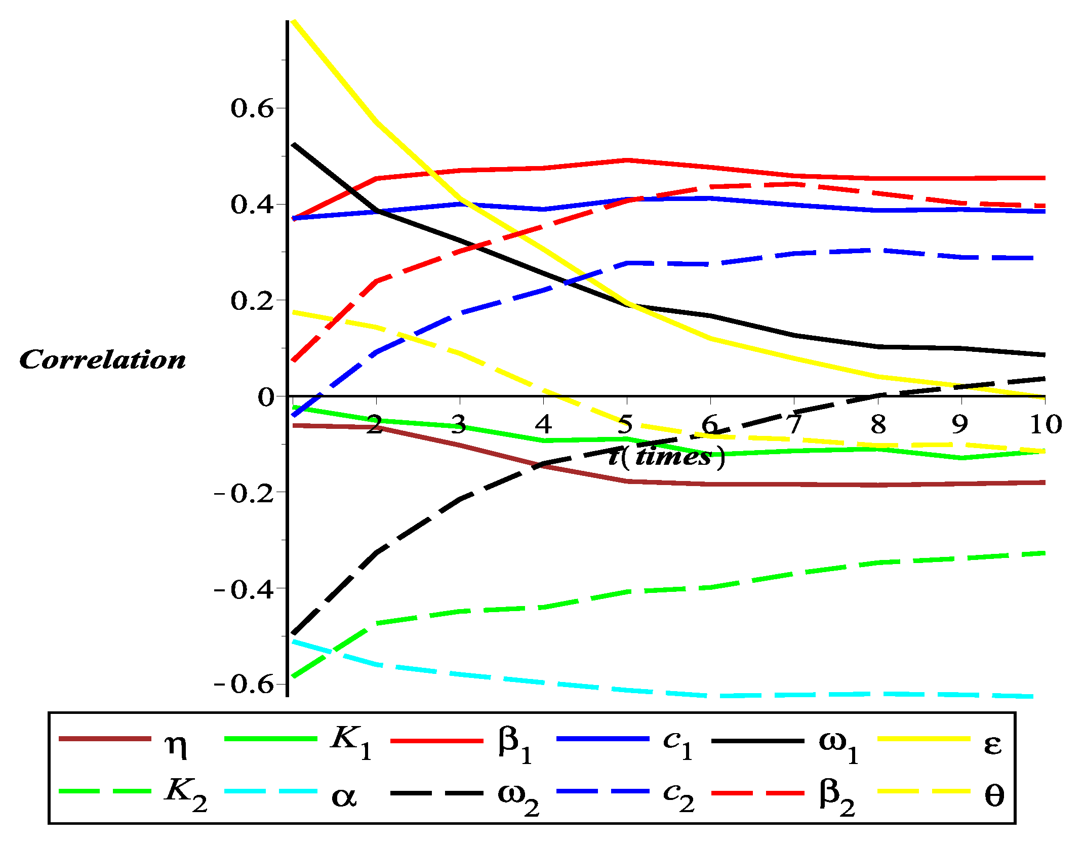
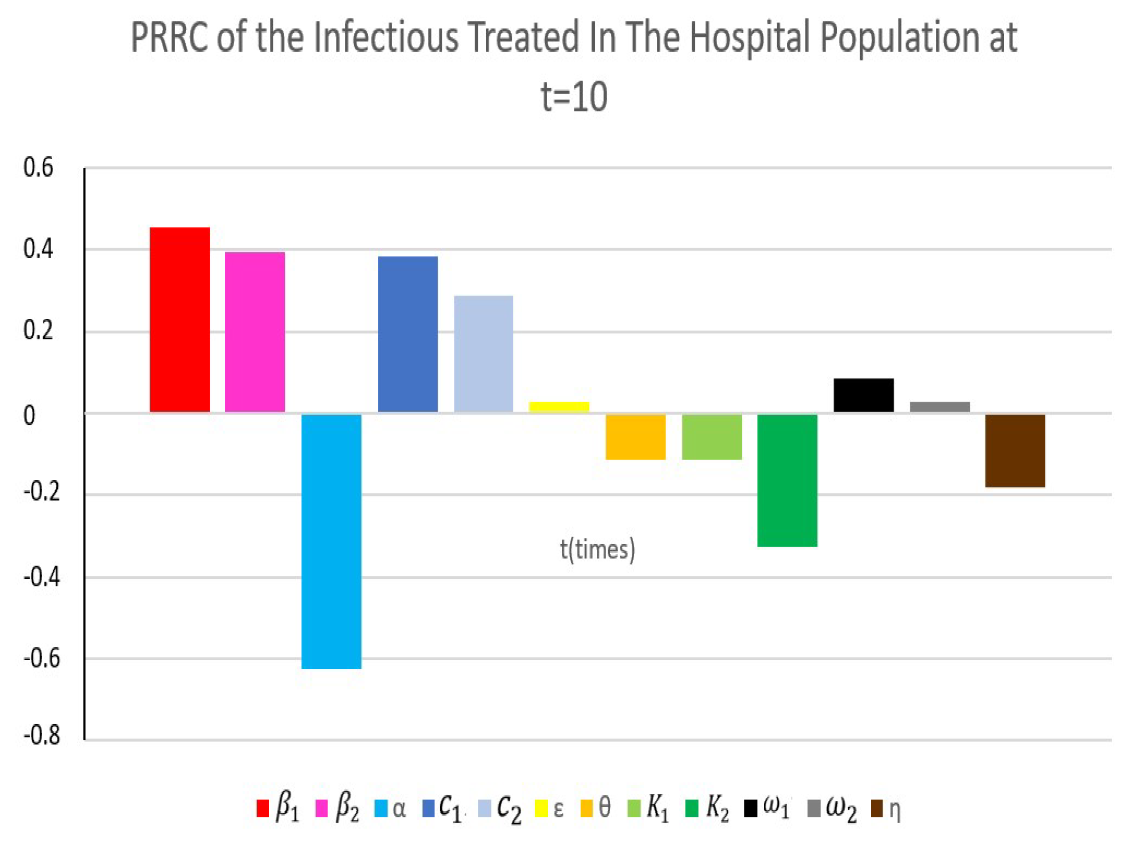
In this subsection, we study the global sensitivity analysis by applying a combination of the Latin Hypercube Sampling (LHS) and the Partial Rank Correlation Coefficient (PRCC). Latin Hypercube Sampling divides the sample interval into a few regions, then takes the same amount of the sample from each part. Hence, the advantage of LHS is that the sample will be distributed fairly in the interval. The data from LHS will be ranked. Then, using PRCC, we can find out the correlation between the parameters and the compartment. Investigating the very impactful and dominant parameters of the system is intended. Hence, all of the parameters in the system were investigated against the increase in infections. For this analysis, our results can be seen in Figure 7 and Figure 8 as well as Figure 9 and Figure 10.
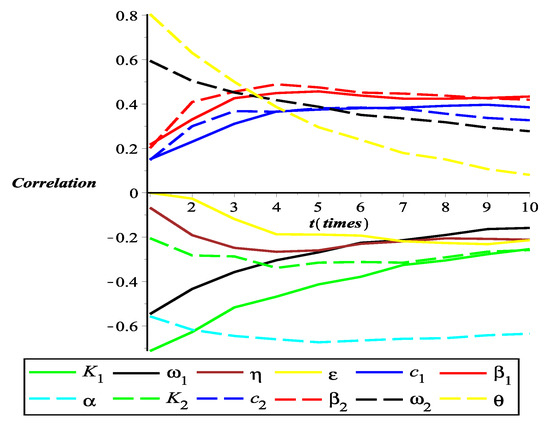
Figure 7.
PRCC of the infectious population treated at home.
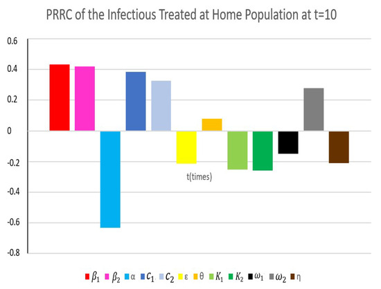
Figure 8.
The bar chart for PRCC of the infectious population treated at home at .
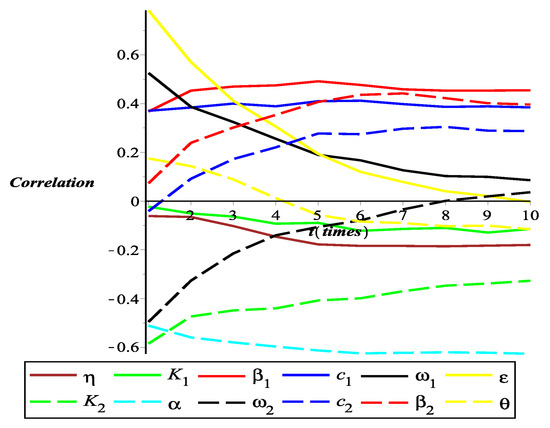
Figure 9.
PRCC of the infectious population treated in the hospital.
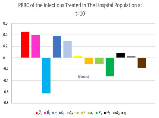
Figure 10.
The bar chart for PRCC of the infectious population treated in the hospital at .
Figure 7 and Figure 8 show that the most sensitive parameter is the half saturated constant , which has a negative correlation. This finding indicates that since the value of increases, the infectious population with treated at home decreased. Meanwhile, the probability of transmission due to contact with an infectious individual with outpatient treatment at home significantly increase on the number of infectious population .
Figure 9 and Figure 10 show that the most sensitive parameter is the half saturated constant , which has a negative correlation. This finding indicates that since the value of increases, the infectious population treated in the hospital decreased. Meanwhile, the probability of transmission due to contact with an infectious individual with care in hospital significantly increase on the number of infectious population .
4.5. Optimal Control
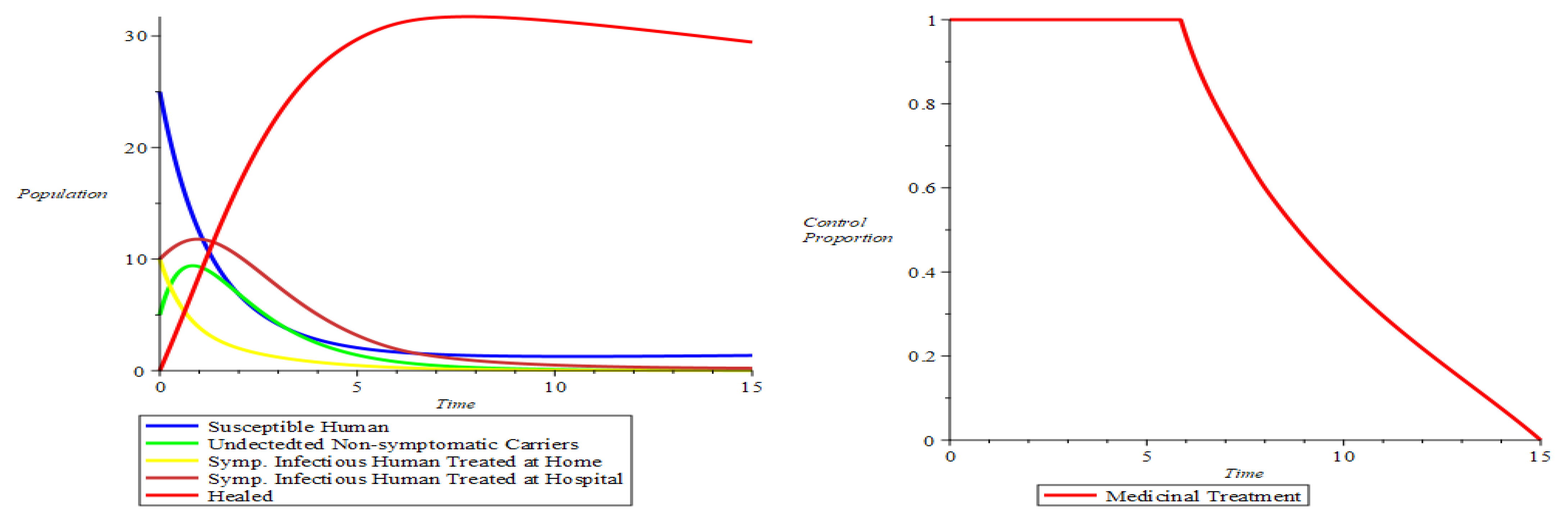
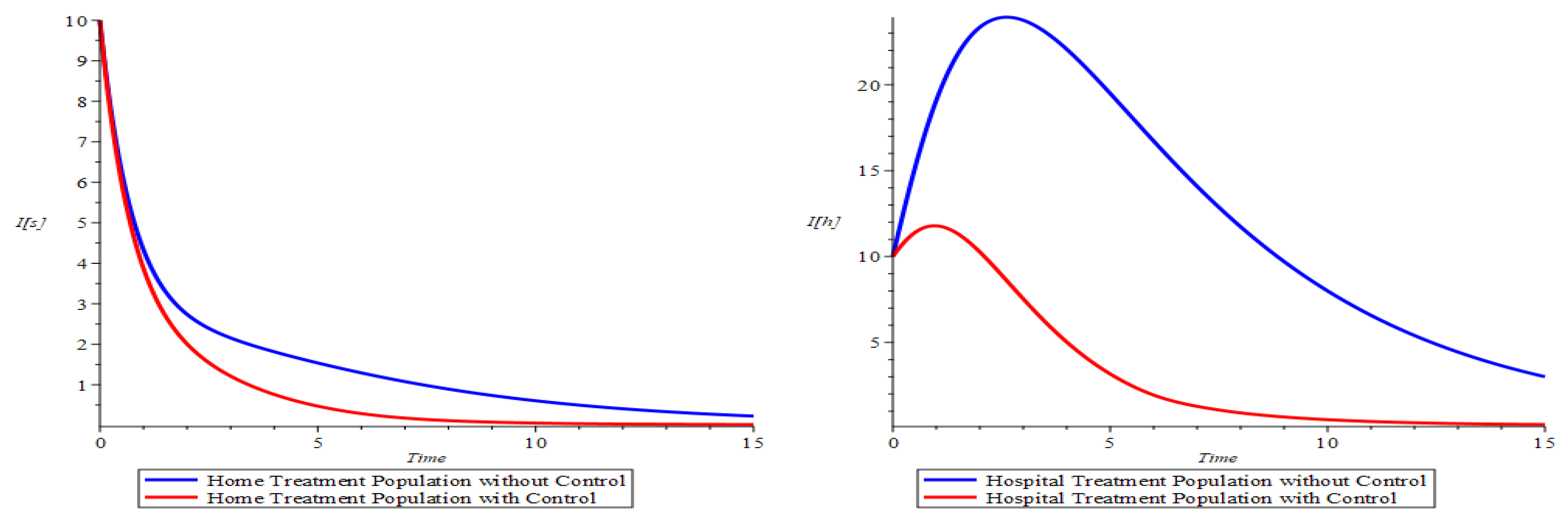
Due to the objective function (8), our goal was to minimize the number of the infected population and the educational effort given. A graph of the dynamical population with its optimal function is shown in the following figure (see Figure 11). It seems that the optimal function has decreased over time, which means that the control has not been occurring all the time because the goal of optimization was achieved when the value of the optimal function was zero.
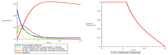
Figure 11.
The impact of optimal control.
Based on Figure 12, the dynamic population with optimal control shows that the infected population, both home treatment and hospital treatment, decreased over time. It means that the goal due to the educational effort as a control in the optimal control problem was successful, which suppressed the infected population and minimized the control. The graph of the dynamic home treatment population shows that at time 1, the difference between the control graph and the without control graph can be seen. Indeed, the graph of the dynamics of hospital treatment populations shows that at the start time, the difference between the control graph and the without control graph can already be seen. All the graphs in Figure 11 show that the educational effort as control has a significant impact on achieving the goals of the optimal control problem.
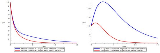
Figure 12.
The impact of optimal control on the compartments and .
5. Conclusions
In this work, a deterministic model for disease outbreaks considering the saturated incidence rate and incomplete treatment was discussed. The population was classified into susceptible , latent/exposed , infected individuals with treatment at home , infected individuals with treatment in hospital , and recovered/healed . By applying a next-generation matrix method, we received the value of , which is a threshold in disease transmission. The special conditions to analyze the existence and also stability of all equilibriums were analyzed.
Our findings show that successful treatment of patients at home can lead to minimizing the prevalence of the disease. In addition, our results also show that the rate of saturated incidence has a crucial role in controlling disease transmission in the population, where the high intervention given influences decreasing the infected population. Another significant role was also influenced by the incomplete treatment received by patients. The high rate of incomplete treatment may increase the population with infectious agents, and people may reenter latent/exposed again. Moreover, we have used control in an educational effort form for the home-treated and hospital-treated populations. The results show that the control process plays an important role in reducing the number of infections significantly. As a consequence of the lack of data for the simulation process of system (1), we hypothesized the parameter values. Despite the unavailability of data to apply to this work, the various assumed parameters used in our model have demonstrated behavior of disease spread. Finally, this model can be applied to study the behavior of disease transmission as long as it has similar behavior patterns.
Author Contributions
Conceptualization; methodology; and software, L.K.B. and N.A. All authors have read and agreed to the published version of the manuscript.
Funding
This work was financially supported by Universitas Padjadjaran, Indonesia, via Post-Doctoral Research Grant Scheme, No. 2474/UN6.3.1/TU.00/2021.
Institutional Review Board Statement
Not applicable.
Informed Consent Statement
Not applicable.
Data Availability Statement
Not applicable.
Acknowledgments
The authors thank Fatuh Inayaturohmat and Sanubari Tansah for their support in this work insightfully. We also thank the reviewers for his/her suggestions, which led to a refinement of paper. We also thank the Provincial Government of Moluccas, including the teachers and staff at SMA Negeri 50 Maluku Tengah for their support to the first author in the Post-Doctoral Program.
Conflicts of Interest
The authors declare no conflict of interest.
Appendix A. The Proof of Analysis for Endemic Point Numerically
The real part of eigenvalues for point are:
This is also confirmed by the fulfillment of the Routh-Hurwitz criteria as follows:
Appendix B. The Proof of Analysis for Non-Endemic Point Numerically
The real part of eigenvalues for point are:
This is also confirmed by the fulfillment of the Routh-Hurwitz criteria as follows:
References
- Caetano, C.; Morgado, M.L.; Patrício, P.; Pereira, J.F.; Nunes, B. Mathematical modelling of the impact of non-pharmacological strategies to control the COVID-19 epidemic in Portugal. Mathematics 2021, 9, 1084. [Google Scholar] [CrossRef]
- Chen, H.; Haus, B.; Mercorelli, P. Extension of SEIR compartmental models for constructive Lyapunov control of COVID-19 and analysis in terms of practical stability. Mathematics 2021, 9, 2076. [Google Scholar] [CrossRef]
- Husniah, H.; Ruhanda, R.; Supriatna, A.K.; Biswas, M.H.A. SEIR mathematical model of convalescent plasma transfusion to reduce COVID-19 disease transmission. Mathematics 2021, 9, 2857. [Google Scholar] [CrossRef]
- Beay, L.K.; Kasbawati; Toaha, S. Effects of human and mosquito migrations on the dynamical behavior of the spread of malaria. AIP Conf. Proc. 2017, 1825, 020006. [Google Scholar] [CrossRef] [Green Version]
- Wongvanich, N.; Tang, I.-M.; Dubois, M.-A.; Pongsumpun, P. Mathematical modeling and optimal control of the Hand Foot Mouth Disease affected by regional residency in Thailand. Mathematics 2021, 9, 2863. [Google Scholar] [CrossRef]
- Islam, M.R.; Peace, A.; Medina, D.; Oraby, T. Integer versus fractional order SEIR deterministic and stochastic models of Measles. Int. J. Environ. Res. Public Health 2020, 17, 2014. [Google Scholar] [CrossRef] [Green Version]
- Saito, M.M.; Imoto, S.; Yamaguchi, R.; Sato, H.; Nakada, H.; Kami, M.; Miyano, S.; Higuchi, T. Extension and verification of the SEIR model on the 2009 Influenza A (H1N1) pandemic in Japan. Math. Biosci. 2013, 246, 47–54. [Google Scholar] [CrossRef]
- Imran, M.; Usman, M.; Dur-e-Ahmad, M.; Khan, A. Transmission dynamics of Zika Fever: A SEIR based model. Differ. Equ. Dyn. Syst. 2021, 29, 463–486. [Google Scholar] [CrossRef]
- Dantas, E.; Tosin, M.; Cunha, A., Jr. Calibration of a SEIR–SEI epidemic model to describe the Zika virus outbreak in Brazil. Appl. Math. Comp. 2018, 338, 249–259. [Google Scholar] [CrossRef] [Green Version]
- Das, K.; Murthy, B.S.N.; Samad, S.A.; Biswas, M.H.A. Mathematical transmission analysis of SEIR Tuberculosis disease model. Sens. Int. 2021, 2, 100120. [Google Scholar] [CrossRef]
- Liu, G.; Chen, J.; Liang, Z.; Peng, Z.; Li, J. Dynamical analysis and optimal control for a SEIR model based on virus mutation in WSNs. Mathematics 2021, 9, 929. [Google Scholar] [CrossRef]
- Coronel, A.; Huancas, F.; Hess, I.; Lozada, E.; Novoa-Muñoz, F. Analysis of a SEIR-KS mathematical model for computer virus propagation in a periodic environment. Mathematics 2020, 8, 761. [Google Scholar] [CrossRef]
- Tuberculosis Chemotherapy Centre. A concurrent comparison of home and sanatorium treatment of Pulmonary Tuberculosis in South India. Bull. World Health Organ. 1959, 21, 51–144. [Google Scholar]
- Suter, F.; Consolaro, E.; Pedroni, S.; Moroni, C.; Pastò, E.; Paganini, M.V.; Pravettoni, G.; Cantarelli, U.; Rubis, N.; Perico, N.; et al. A simple, home-therapy algorithm to prevent hospitalisation for COVID–19 patients: A retrospective observational matched-cohort study. EClinicalMedicine 2021, 37, 100941. [Google Scholar] [CrossRef]
- Consolaro, E.; Suter, F.; Rubis, N.; Pedroni, S.; Moroni, C.; Pastò, E.; Paganini, M.V.; Pravettoni, G.; Cantarelli, U.; Perico, N.; et al. A Home-Treatment Algorithm Based on Anti-inflammatory Drugs to Prevent Hospitalization of Patients With Early COVID-19: A Matched-Cohort Study (COVER 2). Front. Med. 2022, 9, 785785. [Google Scholar] [CrossRef]
- Huo, H.F.; Zou, M.X. Modelling effects of treatment at home on Tuberculosis transmission dynamics. Appl. Math. Model. 2016, 40, 9474–9484. [Google Scholar] [CrossRef]
- Yıldız, T.A.; Karaoğlu, E. Optimal control strategies for Tuberculosis dynamics with exogenous reinfections in case of treatment at home and treatment in hospital. Nonlinear Dyn. 2019, 97, 2643–2659. [Google Scholar] [CrossRef]
- Simorangkir, G.M.; Aldila, D.; Tasman, H. Modelling the effect of hospitalization in Tuberculosis spread. AIP Conf. Proc. 2020, 2264, 020006. [Google Scholar] [CrossRef]
- Zhang, L.; Liu, M.; Hou, Q.; Xie, B. Dynamical analysis of an SEIRS model with incomplete recovery and relapse on networks and its optimal vaccination control. Res. Sq. 2021, 1, 1–30. [Google Scholar] [CrossRef]
- Tudor, D. A deterministic model for herpes infections in human and animal populations. Siam Rev. 1990, 32, 136–139. [Google Scholar] [CrossRef]
- Ullah, I.; Ahmad, S.; Al-Mdallal, Q.; Khan, Z.A.; Khan, H.; Khan, A. Stability analysis of a dynamical model of Tuberculosis with incomplete treatment. Adv. Differ. Equ. 2020, 499, 1–14. [Google Scholar] [CrossRef]
- Neyrolles, O.; Hernández-Pando, R.; Pietri-Rouxel, F.; Fornès, P.; Tailleux, L.; Payán, J.A.B.; Pivert, E.; Bordat, Y.; Aguilar, D.; Prévost, M.-C.; et al. Is adipose tissue a place for Mycobacterium Tuberculosis persistence? PLoS ONE 2006, 1, e43. [Google Scholar] [CrossRef] [PubMed] [Green Version]
- Yang, Y.; Li, J.; Ma, Z.; Liu, L. Global stability of two models with incomplete treatment for Tuberculosis. Chaos Solitons Fractals 2010, 43, 79–85. [Google Scholar] [CrossRef]
- Rahman, M.U.; Arfan, M.; Shah, Z.; Kumam, P.; Shutaywi, M. Nonlinear fractional mathematical model of tuberculosis (TB) disease with incomplete treatment under Atangana-Baleanu derivative. Alex. Eng. J. 2021, 60, 2845–2856. [Google Scholar] [CrossRef]
- Jafari, M.; Kheiri, H.; Jabbari, A. Backward bifurcation in a fractional-order and two-patch model of tuberculosis epidemic with incomplete treatment. Int. J. Biomath. 2021, 14, 2150007. [Google Scholar] [CrossRef]
- Suryanto, A.; Darti, I. On the nonstandard numerical discretization of SIR epidemic model with a saturated incidence rate and vaccination. AIMS Math. 2020, 6, 141–155. [Google Scholar] [CrossRef]
- Thirthar, A.A.; Naji, R.K.; Bozkurt, F.; Yousef, A. Modeling and analysis of an SI1I2R epidemic model with nonlinear incidence and general recovery functions of I1. Chaos Solitons Fractals 2021, 145, 110746. [Google Scholar] [CrossRef]
- Li, L.; Sun, C.; Jia, J. Optimal control of a delayed SIRC epidemic model with saturated incidence rate. Optim. Control Appl. Meth. 2018, 40, 367–374. [Google Scholar] [CrossRef]
- Bentaleb, D.; Harroudi, S.; Amine, S.; Allali, K. Analysis and optimal control of a multistrain SEIR epidemic model with saturated incidence rate and treatment. Differ. Equ. Dyn. Syst. 2020, 1, 1–17. [Google Scholar] [CrossRef]
- Khan, M.A.; Khan, Y.; Islam, S. Complex dynamics of an SEIR epidemic model with saturated incidence rate and treatment. Phys. A 2018, 493, 210–227. [Google Scholar] [CrossRef]
- Mushayabasa, S. A simple epidemiological model for typhoid with saturated incidence rate and treatment effect. Int. J. Math. Comput. Sci. 2012, 6, 688–695. [Google Scholar] [CrossRef]
- Alshammari, F.S.; Khan, M.A. Dynamic behaviors of a modified SIR model with nonlinear incidence and recovery rates. Alex. Eng. J. 2021, 60, 2997–3005. [Google Scholar] [CrossRef]
- Hussain, G.; Khan, A.; Zahri, M.; Zaman, G. Stochastic permanence of an epidemic model with a saturated incidence rate. Chaos Solitons Fractals 2020, 139, 110005. [Google Scholar] [CrossRef]
- Okuonghae, D. Backward bifurcation of an epidemiological model with saturated incidence, isolation and treatment functions. Qual. Theory Dyn. Syst. 2020, 18, 413–440. [Google Scholar] [CrossRef]
- Baba, I.A.; Abdulkadir, R.A.; Esmaili, P. Analysis of tuberculosis model with saturated incidence rate and optimal control. Physica A 2020, 540, 123237. [Google Scholar] [CrossRef]
- Mengistu, A.K.; Witbooi, P.J. Mathematical analysis of TB model with vaccination and saturated incidence rate. Abstr. Appl. Anal. 2020, 2020, 6669997. [Google Scholar] [CrossRef]
- Indrayani, S.W.; Kusumawinahyu, W.M.; Trisilowati. Dynamical Analysis on the model of Tuberculosis spread with vaccination and saturated incident rate. IOP Conf. Ser. Mater. Sci. Eng. 2019, 546, 052032. [Google Scholar] [CrossRef]
- Sutimin; Herdiana, R.; Soelistyo U, R.H.; Permatasari, A.H. Stability analysis of Tuberculosis epidemic model with saturated infection force. E3S Web Conf. 2020, 202, 12023. [Google Scholar] [CrossRef]
- Khan, T.; Zaman, G. Classification of different Hepatitis B infected individuals with saturated incidence rate. SpringerPlus 2016, 5, 1082. [Google Scholar] [CrossRef] [Green Version]
- Andayani, P. The effect of social media for a Zika virus transmission with Beddington DeAngelis incidence rate: Modeling and analysis. AIP Conf. Proc. 2019, 2183, 090003. [Google Scholar] [CrossRef]
- Algehyne, E.A.; Din, R. On global dynamics of COVID-19 by using SQIR type model under non-linear saturated incidence rate. Alex. Eng. J. 2021, 60, 393–399. [Google Scholar] [CrossRef]
- Omame, A.; Okuonghae, D. A co-infection model for oncogenic Human Papillomavirus and Tuberculosis with optimal control and Cost-Effectiveness analysis. Optim. Control Appl. Meth. 2021, 42, 1081–1101. [Google Scholar] [CrossRef]
- Samui, P.; Mondal, J.; Khajanchi, S. A mathematical model for COVID-19 transmission dynamics with a case study of India. Chaos Solitons Fractals 2020, 140, 110173. [Google Scholar] [CrossRef] [PubMed]
- Nur, W.; Trisilowati; Suryanto, A.; Kusumawinahyu, W.M. Schistosomiasis model incorporating snail predator as biological control agent. Mathematics 2021, 9, 1858. [Google Scholar] [CrossRef]
- Anggriani, N.; Beay, L.K. Modeling of COVID–19 spread with self–isolation at home and hospitalized classes. Results Phys. 2022, 36, 105378. [Google Scholar] [CrossRef]

Publisher’s Note: MDPI stays neutral with regard to jurisdictional claims in published maps and institutional affiliations. |
© 2022 by the authors. Licensee MDPI, Basel, Switzerland. This article is an open access article distributed under the terms and conditions of the Creative Commons Attribution (CC BY) license (https://creativecommons.org/licenses/by/4.0/).