Further Study on C-Eigenvalue Inclusion Intervals for Piezoelectric Tensors

Abstract

The C-eigenpair of piezoelectric tensors finds applications in the area of the piezoelectric effect and converse piezoelectric effect. In this paper, we provide some characterizations of C-eigenvectors by exploring the structure of piezoelectric tensors, and establish sharp C-eigenvalue inclusion intervals via Cauchy–Schwartz inequality. Further, we propose the lower and upper bounds of the largest C-eigenvalue and evaluate the efficiency of the best rank-one approximation of piezoelectric tensors. Numerical examples are proposed to verify the efficiency of the obtained results.

1. Introduction

Third-order tensors play an important role in physics and engineering, such as in solid crystal study [1,2,3,4] and liquid crystal study [1,5,6]. We know that piezoelectric tensors are the most well-known tensor among third-order tensors and come from applications in the piezoelectric effect and converse piezoelectric effect in solid crystals from [1,2,7].

Definition 1.

A third-order n dimensional real tensor $\mathcal{A}=(a_{ijk})$ is called a piezoelectric tensor, if the later two indices of $\mathcal{A}$ are symmetric, i.e., $a_{ijk}=a_{ikj}$ for all $j,k\in N$, where $N=\{1,2,\dots ,n\}.$

In order to explore the properties of the piezoelectric effect, Chen et al. [8] introduced the following C-eigenpair.

Definition 2.

For piezoelectric tensor $\mathcal{A}=(a_{ijk})\in {\mathbb{R}}^{n\times n\times n}$, if there exists a scalar $\lambda \in \mathbb{R}$ and vectors $x,y\in {\mathbb{R}}^n$ such that

$$\begin{array}{c}\hfill \mathcal{A}yy=\lambda x,x\mathcal{A}y=\lambda y,x^{\top }x=1,y^{\top }y=1,\end{array}$$

(1)

where $\mathcal{A}yy\in {\mathbb{R}}^n$ and $x\mathcal{A}y\in {\mathbb{R}}^n$ with the i-th and the k-th entries

$$\begin{array}{c}\hfill {(\mathcal{A}yy)}_i=\sum _{j,k\in N}{a}_{ijk}{y}_j{y}_k,{(x\mathcal{A}y)}_k=\sum _{i,j\in N}{a}_{ijk}{x}_i{y}_j,\end{array}$$

then λ is called a C-eigenvalue of $\mathcal{A},and$ x and y are called associated left and right C-eigenvectors, respectively. For simplicity, $(\lambda ,x,y)$ is called a C-eigenpair of $\mathcal{A}.$

To investigate the existence and properties of C-eigenpairs of a piezoelectric-type tensor, we recall the following theorem established in [8].

Lemma 1.

[Theorem 2.3 of [8]] Let $\mathcal{A}$ be a piezoelectric-type tensor. Then,

(i) 

There exist C-eigenvalues of $\mathcal{A}$ and associated left and right C-eigenvectors.

(ii) 

Suppose that $\lambda ,x$ and y are a C-eigenvalue and its associated left and right C-eigenvectors of $\mathcal{A}$, respectively. Then

$$\begin{array}{c}\hfill \lambda =x\mathcal{A}yy.\end{array}$$

Further, $(\lambda ,x,-y)$, $(-\lambda ,-x,y)$ and $(-\lambda ,-x,-y)$ are also C-eigenpairs of tensor $\mathcal{A}$.

(iii) 

Denote the largest C-eigenvalue of $\mathcal{A}$ and its associated left and right C-eigenvectors as ${\lambda }^{*},x^{*},y^{*},$ respectively. Then

$$\begin{array}{c}\hfill {\lambda }^{*}=max\{x\mathcal{A}yy:x^{\top }x=1and{y}^{\top }y=1\}.\end{array}$$

Further, ${\lambda }^{*}{x}^{*}\circ y^{*}\circ y^{*}$ forms the best rank-one piezoelectric-type approximation of $\mathcal{A}.$

As we know, the largest C-eigenvalue of a piezoelectric tensor has concrete physical meaning which determines the highest piezoelectric coupling constant [1]. In view of the significance of the largest C-eigenvalue, effective algorithms have been implemented [9,10,11]. As pointed out by Chen et al. [8], the number of C-eigenvalues is equal to $\frac{3^n-1}{2}$ when a piezoelectric tensor has finitely many equivalence classes of C-eigenvalues; it is very costly to compute the largest C-eigenvalue or all C-eigenvalues for a high-dimensional piezoelectric tensor. Thus, some researchers turned to giving an interval to locate all C-eigenvalues of piezoelectric tensors. Li et al. [12] first gave C-eigenvalue inclusion intervals to locate the C-eigenvalues of piezoelectric tensors via the S-partition method. Improved results can be found in [13,14,15,16]. As a special type of third-order tensor, piezoelectric tensors have unique properties on C-eigenvectors. For instance, for the right C-eigenvector y, the fact that $\underset{i\ne j\in N}{max}|y_i||y_j|\le \frac{1}{2}$ holds. Therefore, if we perform an in-depth characterization of C-eigenvectors and the structure of a piezoelectric tensor, we shall establish sharp C-eigenvalue inclusion intervals. This constitutes the first motivation of the paper.

It is well known that the best rank-one approximation of a tensor has numerous applications in higher-order statistical data analysis [17,18,19,20]. For piezoelectric tensor $\mathcal{A}=(a_{ijk}),$ its best rank-one approximation is to find a scalar $\lambda$ and vectors $x,y$ which minimize the following optimization problem:

$$\begin{array}{c}\hfill \underset{\lambda \in \mathbb{R},x^{\top }x=1,y^{\top }y=1}{min}||\mathcal{A}-\lambda x\circ y\circ {y||}_F,\end{array}$$

where ${||\mathcal{A}||}_F:=\sqrt{{\displaystyle \sum _{i,j,k\in N}}{a}_{ijk}^2},$ and “∘” means the outer product and $\lambda x\circ y\circ y$ is a rank-one tensor [6,8]. Further, Chen et al. [8] showed that the largest C-eigenvalue ${\lambda }^{*}$ and its C-eigenvectors $(x^{*},y^{*})$ form the best rank-one piezoelectric-type approximation of $\mathcal{A},$ i.e.,

$$\begin{array}{c}\hfill \underset{\lambda \in \mathbb{R},x^{\top }x=1,y^{\top }y=1}{min}||\mathcal{A}-\lambda x\circ y\circ {y||}_F=||\mathcal{A}-{\lambda }^{*}{x}^{*}\circ y^{*}\circ y^{*}{||}_F=\sqrt{{||\mathcal{A}||}_F^2-{{\lambda }^{*}}^2}.\end{array}$$

Thus, we obtain the quotient of the residual of a symmetric best rank-one approximation of piezoelectric tensor $\mathcal{A}$ as follows:

$$\begin{array}{c}\hfill \omega =\frac{\sqrt{{||\mathcal{A}||}_F-{{\lambda }^{*}}^2}}{{||\mathcal{A}||}_F},\end{array}$$

which can be used to evaluate the efficiency of the best rank-one approximation. When we extract tensor information with the best rank-one approximation, a natural problem is how to quickly evaluate the efficiency of information extraction. Obviously, the smaller $\omega$ is, the greater the efficiency of the best rank-one approximation. Therefore, we want to estimate the upper and lower bounds of the largest C-eigenvalue to evaluate the efficiency of the best rank-one approximation of piezoelectric tensors, which represents the second motivation of the paper.

The remainder of the paper is organized as follows. In Section 2, we first recall some fundamental existing results. By virtue of components of the left and right C-eigenvector, we establish new C-eigenvalue inclusion intervals of piezoelectric tensors, and show that these C-eigenvalue intervals are sharper than some existing C-eigenvalue intervals. In Section 3, we use bound estimations of the largest C-eigenvalue to evaluate the efficiency of the best rank-one approximation of piezoelectric tensors. The validity of the obtained results is tested by some examples.

2. C-eigenvalue Inclusion Intervals for Piezoelectric Tensors

In this section, we shall establish some sharp C-eigenvalue inclusion intervals based on the exploration of its eigenvectors, and show that these C-eigenvalue inclusion intervals improve some existing results [12,13,14,16]. To proceed, we recall the C-eigenvalue inclusion intervals established by [12].

Lemma 2.

For piezoelectric tensor $\mathcal{A}=(a_{ijk})\in {\mathbb{R}}^{n\times n\times n}$ and its C-eigenvalue λ, it holds that

$$\begin{array}{c}\hfill \lambda \in [-\rho ,\rho ],\end{array}$$

where $\rho =\underset{i,k\in N}{max}\sqrt{R_i^{(1)}(\mathcal{A})R_k^{(3)}(\mathcal{A})},$ $R_i^{(1)}(\mathcal{A})={\displaystyle \sum _{j,k\in N}}|a_{ijk}|$ and $R_k^{(3)}(\mathcal{A})={\displaystyle \sum _{i,j\in N}}|a_{ijk}|.$

From Theorem 2.3 of [8], we deduce that $-\lambda$ is a C-eigenvalue if $\lambda$ is a C-eigenvalue. Hence, the C-eigenvalue inclusion interval is symmetric about the origin. Before proceeding further, we need to establish the following lemma on the C-eigenvector.

Lemma 3.

For unit vector $y\in {\mathbb{R}}^n,$ it holds that $\underset{i,j\in N,i\ne j}{max}|y_i||y_j|\le \frac{1}{2}.$

Proof. 

For all $i\ne j\in N$, it follows from $2|y_i||y_j|\le y_i^2+y_j^2$ that

$$2|y_i||y_j|\le y_i^2+y_j^2\le y_1^2+y_2^2+\dots +y_n^2=1,$$

which implies $\underset{i,j\in N,i\ne j}{max}|y_i||y_j|\le \frac{1}{2}.$□

Theorem 1.

Let λ be a C-eigenvalue of piezoelectric tensor $\mathcal{A}=(a_{ijk})\in {\mathbb{R}}^{n\times n\times n}$. Then,

$$\begin{array}{c}\hfill \lambda \in [-\delta ,\delta ],\end{array}$$

where $\delta =\underset{i,k\in N}{max}\sqrt{({\alpha }_i+{\beta }_i)R_k^{(3)}(\mathcal{A})},$ ${\alpha }_i=\underset{j\in N}{max}\{|a_{ijj}|\},{\beta }_i=\frac{1}{2}{\displaystyle \sum _{j,k\in N,j\ne k}}|a_{ijk}|$ and $R_k^{(3)}(\mathcal{A})={\displaystyle \sum _{i,j\in N}}|a_{ijk}|.$

Proof. 

Let $(\lambda ,x,y)$ be a C-eigenpair of the piezoelectric tensor $\mathcal{A}$. Set $|x_p|=\underset{i\in N}{max}|x_i|$ and $|y_q|=\underset{i\in N}{max}|y_i|$. Since $x^{\top }x=1$ and $y^{\top }y=1,$ then $0<|x_p|\le 1$ and $0<|y_q|\le 1$. By the p-th equation of $\mathcal{A}yy=\lambda x$ in (1), we have

$$\begin{array}{c}\hfill \lambda x_p=\sum _{j,k\in N}{a}_{pjk}{y}_j{y}_k,\end{array}$$

(2)

$$\begin{array}{c}\hfill \lambda x_p=\sum _{j,k\in N,j=k}{a}_{pjj}{y}_j{y}_j+\sum _{j,k\in N,j\ne k}{a}_{pjk}{y}_j{y}_k.\end{array}$$

(3)

By the definitions of ${\alpha }_i,{\beta }_i$ and Lemma 3, we obtain

$$\begin{array}{cc}\hfill |\lambda ||x_p|& \hfill \le \sum _{j\in N}|a_{pjj}||y_j||y_j|+\sum _{j,k\in N,j\ne k}|a_{pjk}||y_j||y_k|\hfill \\ \hfill & \hfill \le {\alpha }_p\sum _{j\in N}|y_j||y_j|+\frac{1}{2}\sum _{j,k\in N,j\ne k}|a_{pjk}|={\alpha }_p+{\beta }_p,\hfill \end{array}$$

which shows

$$\begin{array}{c}\hfill |\lambda ||x_p|\le {\alpha }_p+{\beta }_p.\end{array}$$

(4)

On the other hand, the q-th equation of $x\mathcal{A}y=\lambda y$ in (1) yields

$$\begin{array}{c}\hfill \lambda y_q=\sum _{i,j\in N}{a}_{ijq}{x}_i{y}_j\mathrm{and}|\lambda ||y_q|\le \sum _{i,j\in N}|a_{ijk}||x_i||y_j|.\end{array}$$

Since $|x_p|=\underset{i\in N}{max}|x_i|$ and $|y_q|=\underset{i\in N}{max}|y_i|$, we have

$$\begin{array}{c}\hfill |\lambda ||y_q|\le \sum _{i,j\in N}|a_{ijq}||x_p||y_q|,\end{array}$$

which implies

$$\begin{array}{c}\hfill |\lambda |\le \sum _{i,j\in N}|a_{ijq}||x_p|=R_q^{(3)}(\mathcal{A})|x_p|.\end{array}$$

(5)

Multiplying (4) with (5) yields

$$\begin{array}{c}\hfill {|\lambda |}^2|x_p|\le ({\alpha }_p+{\beta }_p)R_q^{(3)}(\mathcal{A})|x_p|\mathrm{and}|\lambda |\le \sqrt{({\alpha }_p+{\beta }_p)R_q^{(3)}(\mathcal{A})}.\end{array}$$

Further,

$$\begin{array}{c}\hfill |\lambda |\le \underset{i,k\in N}{max}\sqrt{({\alpha }_i+{\beta }_i)R_k^{(3)}(\mathcal{A})}.\end{array}$$

□

Now, we give a theoretical comparison between Theorem 1 and Theorem 1 of [12].

Remark 1.

Noting that

$${\alpha }_i=\underset{j\in N}{max}|a_{ijj}|\le \sum _{j=k\in N}|a_{ijj}|and{\beta }_i=\frac{1}{2}\sum _{j\ne k\in N}|a_{ijk}|\le \sum _{j\ne k\in N}|a_{ijk}|,$$

we deduce that

$$\begin{array}{c}\hfill {\alpha }_i+{\beta }_i\le \sum _{j\in N}|a_{ijj}|+\sum _{j\ne k\in N}|a_{ijk}|=R_i^{(1)}(\mathcal{A}).\end{array}$$

Hence,

$$\begin{array}{c}\hfill \underset{i,k\in N}{max}\sqrt{({\alpha }_i+{\beta }_i)R_k^{(3)}(\mathcal{A})}\le \underset{i,k\in N}{max}\sqrt{R_i^{(1)}(\mathcal{A})R_k^{(3)}(\mathcal{A})}.\end{array}$$

Thus, the interval $[-\delta ,\delta ]$ in Theorem 1 captures all C-eigenvalues of piezoelectric tensors more precisely than the interval $[-\rho ,\rho ]$ given in [12].

It is well known that C-eigenvalues are invariant under orthogonal transformations, i.e., for C-eigenpair $(\lambda ,x,y)$ of piezoelectric tensor $\mathcal{A}$ and orthogonal matrix Q, $\mathcal{A}{Q}^3$ is also a piezoelectric tensor [8,12], and $(\lambda ,Qx,Qy)$ is also a C-eigenvalue of tensor $\mathcal{A}{Q}^3$, where

$$\begin{array}{c}\hfill {(\mathcal{A}{Q}^3)}_{rst}=\sum _{i,j,k\in N}{a}_{ijk}{q}_{ir}{q}_{js}{q}_{kt}.\end{array}$$

Hence, Li et al. [12] derived the following new C-eigenvalue interval for a piezoelectric tensor:

$$\begin{array}{c}\hfill \lambda \in [-\underset{Q\in {\mathcal{Q}}^{n\times n}}{min}{\rho }_Q,\underset{Q\in {\mathcal{Q}}^{n\times n}}{min}{\rho }_Q],\end{array}$$

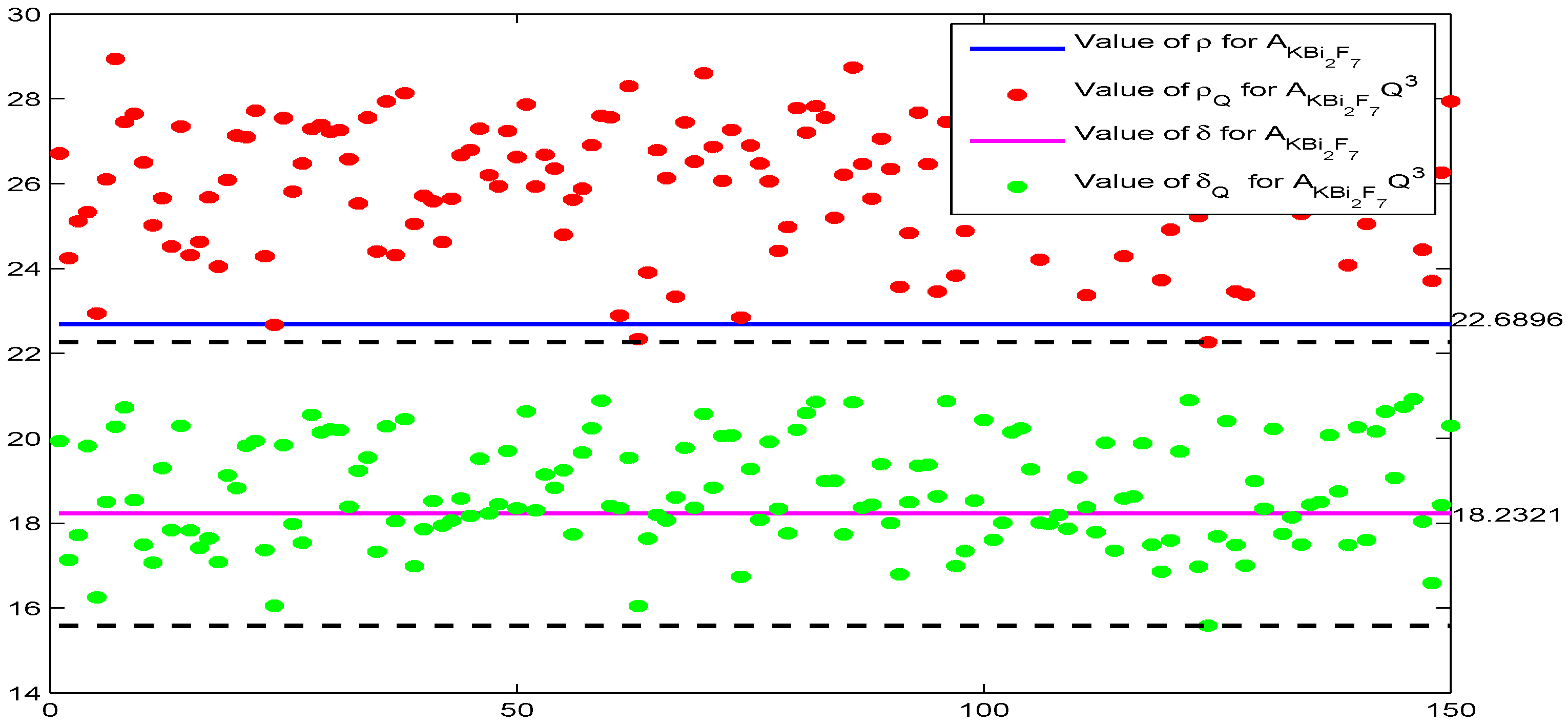
where ${\rho }_Q=\underset{i,k\in N}{max}{\left\{R_i^{(1)}(\mathcal{A}{Q}^3)R_k^{(3)}(\mathcal{A}{Q}^3)\right\}}^{\frac{1}{2}}$ and ${\mathcal{Q}}^{n\times n}$ denotes the orthogonal matrix sets. However, the interval $[-\delta ,\delta ]$ given in Theorem 1 may not be invariant under orthogonal transformation, as shown below. Consider the piezoelectric tensor ${\mathcal{A}}_{KB{i}_2{F}_7}$ in [8,21] with its nonzero entries

$$\begin{array}{cc}\hfill & a_{111}=12.64393,a_{122}=1.08802,a_{133}=4.14350,a_{123}=1.59052,\hfill \\ \hfill & a_{113}=1.96801,a_{112}=0.22465,a_{211}=2.59187,a_{222}=0.08263,\hfill \\ \hfill & a_{233}=0.81041,a_{223}=0.51165,a_{213}=0.71432,a_{212}=0.10570,\hfill \\ \hfill & a_{311}=1.51254,a_{322}=0.68235,a_{333}=-0.23019,a_{323}=0.19013,\hfill \\ \hfill & a_{313}=0.39030,a_{312}=0.08381.\hfill \end{array}$$

For orthogonal matrix

$$\begin{array}{c}\hfill Q=\left(\begin{array}{ccc}\frac{\sqrt{2}}{2}& 0& \frac{\sqrt{2}}{2}\\ 0& 1& 0\\ -\frac{\sqrt{2}}{2}& 0& \frac{\sqrt{2}}{2}\end{array}\right),\end{array}$$

we have

$$\begin{array}{c}\hfill {\delta }_Q=\underset{i,k\in N}{max}\sqrt{({\alpha }_i(\mathcal{A}{Q}^3)+{\beta }_i(\mathcal{A}{Q}^3))R_k^{(3)}(\mathcal{A}{Q}^3)}=18.7823,\end{array}$$

$$\begin{array}{c}\hfill \delta =\underset{i,k\in N}{max}\sqrt{({\alpha }_i+{\beta }_i)R_k^{(3)}(\mathcal{A})}=18.2321.\end{array}$$

Further, taking 150 orthogonal matrices Q generated by the MATLAB code

$$\begin{array}{c}\hfill n=3,Qrand=rand(n,n),Q=orth(Qrand),\end{array}$$

we could obtain various values of $\delta$ and ${\delta }_Q$ for ${\mathcal{A}}_{KB{i}_2{F}_7}$ and ${\mathcal{A}}_{KB{i}_2{F}_7}{Q}^3$; see Figure 1.

Figure 1. Comparisons among $\rho$ and ${\rho }_Q$ in [12] and $\delta$ and ${\delta }_Q$ for ${\mathcal{A}}_{KB{i}_2{F}_7}$ and ${\mathcal{A}}_{KB{i}_2{F}_7}{Q}^3$.

Obviously, there are some orthogonal matrices Q such that ${\delta }_Q$ in Theorem 1 becomes smaller. From the arbitrariness of orthogonal matrix Q, for C-eigenvalue $\lambda$ of piezoelectric tensor $\mathcal{A},$ it holds that $\lambda \in [-\underset{Q\in {\mathcal{Q}}^{n\times n}}{min}{\delta }_Q,\underset{Q\in {\mathcal{Q}}^{n\times n}}{min}{\delta }_Q].$

Corollary 1.

Let ${\lambda }^{*}$ be the largest C-eigenvalue of piezoelectric tensor $\mathcal{A}=(a_{ijk})\in {\mathbb{R}}^{n\times n\times n}$. Then,

$$\begin{array}{c}\hfill {\lambda }^{*}\le \underset{Q\in {\mathcal{Q}}^{n\times n}}{min}{\delta }_Q\le \delta ,\end{array}$$

where ${\delta }_Q=\underset{i,k\in N}{max}\sqrt{({\alpha }_i(\mathcal{A}{Q}^3)+{\beta }_i(\mathcal{A}{Q}^3))R_k^{(3)}(\mathcal{A}{Q}^3)}.$

By ${\displaystyle \sum _{j\in N}}{y}_j^2=1$ and Cauchy–Schwartz inequality, we are in the position to establish the following theorems.

Theorem 2.

Let λ be a C-eigenvalue of piezoelectric tensor $\mathcal{A}=(a_{ijk})\in {\mathbb{R}}^{n\times n\times n}$. Then

$$\begin{array}{c}\hfill \lambda \in [-\eta ,\eta ],\end{array}$$

where $\eta =\underset{i,k\in N}{max}\sqrt{r_i^{(1)}(\mathcal{A})r_k^{(3)}(\mathcal{A})},$ $r_i^{(1)}(\mathcal{A})=\sqrt{{\displaystyle \sum _{j\in N}}({\displaystyle \sum _{k\in N}}|a_{ijk}{|)}^2}$ and $r_k^{(3)}(\mathcal{A})=$$\sqrt{{\displaystyle \sum _{j\in N}}({\displaystyle \sum _{i\in N}}|a_{ijk}{|)}^2}.$

Proof. 

Let $(\lambda ,x,y)$ be a C-eigenpair of the piezoelectric tensor $\mathcal{A}$. Setting $|x_p|=\underset{i\in N}{max}|x_i|$ and $|y_q|=\underset{i\in N}{max}|y_i|$, we obtain $0<|x_p|\le 1$ and $0<|y_q|\le 1.$ By the p-th equation of $\mathcal{A}yy=\lambda x$ in (1), we have

$$\begin{array}{c}\hfill \lambda x_p=\sum _{j,k\in N}{a}_{pjk}{y}_j{y}_k\end{array}$$

and

$$\begin{array}{cc}|\lambda ||x_p|\hfill & \hfill \le \sum _{j,k\in N}|a_{pjk}||y_j||y_k|\le \sum _{j,k\in N}|a_{pjk}||y_j||y_q|\\ \hfill & =\sum _{j\in N}\sum _{k\in N}|a_{pjk}||y_j||y_q|\hfill \\ \hfill & \le \sqrt{\sum _{j\in N}(\sum _{k\in N}|a_{pjk}{|)}^2}\sqrt{\sum _{j\in N}{|y_j|}^2}|y_q|\hfill \\ \hfill & =\sqrt{\sum _{j\in N}(\sum _{k\in N}|a_{pjk}{|)}^2}|y_q|,\hfill \end{array}$$

(6)

where the third inequality uses Cauchy–Schwartz inequality and the second equality follows from ${\displaystyle \sum _{j\in N}}{|y_j|}^2=1$.

On the other hand, recalling the q-th equation of $x\mathcal{A}y=\lambda y$ in (1), one has

$$\begin{array}{c}\hfill \lambda y_q=\sum _{i,j\in N}{a}_{ijq}{x}_i{y}_j,|\lambda ||y_q|\le \sum _{i,j\in N}|a_{ijq}||x_i||y_j|.\end{array}$$

Since $|x_p|=\underset{i\in N}{max}|x_i|$ and $|y_q|=\underset{i\in N}{max}|y_i|$, we have

$$\begin{array}{cc}\hfill |\lambda ||y_q|& \le \sum _{i,j\in N}|a_{ijq}||x_i||y_j|\le \sum _{i,j\in N}|a_{ijq}||y_j||x_p|\hfill \\ \hfill & \le \sqrt{\sum _{j\in N}(\sum _{i\in N}|a_{ijq}{|)}^2}\sqrt{\sum _{j\in N}{|y_j|}^2}|x_p|\hfill \\ \hfill & =\sqrt{\sum _{j\in N}(\sum _{i\in N}|a_{ijq}{|)}^2}|x_p|,\hfill \end{array}$$

(7)

where the third inequality uses the Cauchy–Schwartz inequality and the equality follows from ${\displaystyle \sum _{j\in N}}{|y_j|}^2=1.$ Multiplying (6) with (7) yields

$$\begin{array}{c}\hfill {|\lambda |}^2|x_p||y_q|\le \sqrt{\sum _{j\in N}(\sum _{k\in N}|a_{pjk}{|)}^2}\sqrt{\sum _{j\in N}(\sum _{i\in N}|a_{ijq}{|)}^2}|y_q||x_p|\end{array}$$

and

$$\begin{array}{c}\hfill |\lambda |\le \{(\sum _{j\in N}(\sum _{k\in N}|a_{pjk}{|)}^2)(\sum _{j\in N}(\sum _{i\in N}|a_{ijq}{|)}^2{)\}}^{\frac{1}{4}}.\end{array}$$

By the definitions of $r_i^{(1)}(\mathcal{A})$ and $r_k^{(3)}(\mathcal{A}),$ we obtain

$$|\lambda |\le \underset{i,k\in N}{max}\{(\sum _{j\in N}(\sum _{k\in N}|a_{ijk}{|)}^2)(\sum _{j\in N}(\sum _{i\in N}|a_{ijk}{|)}^2{)\}}^{\frac{1}{4}}=\underset{i,k\in N}{max}\sqrt{r_i^{(1)}(\mathcal{A})r_k^{(3)}(\mathcal{A})}.$$

□

Now, we make another theoretical comparison of the upper bounds given in Theorem 2 and Theorem 1 in [12].

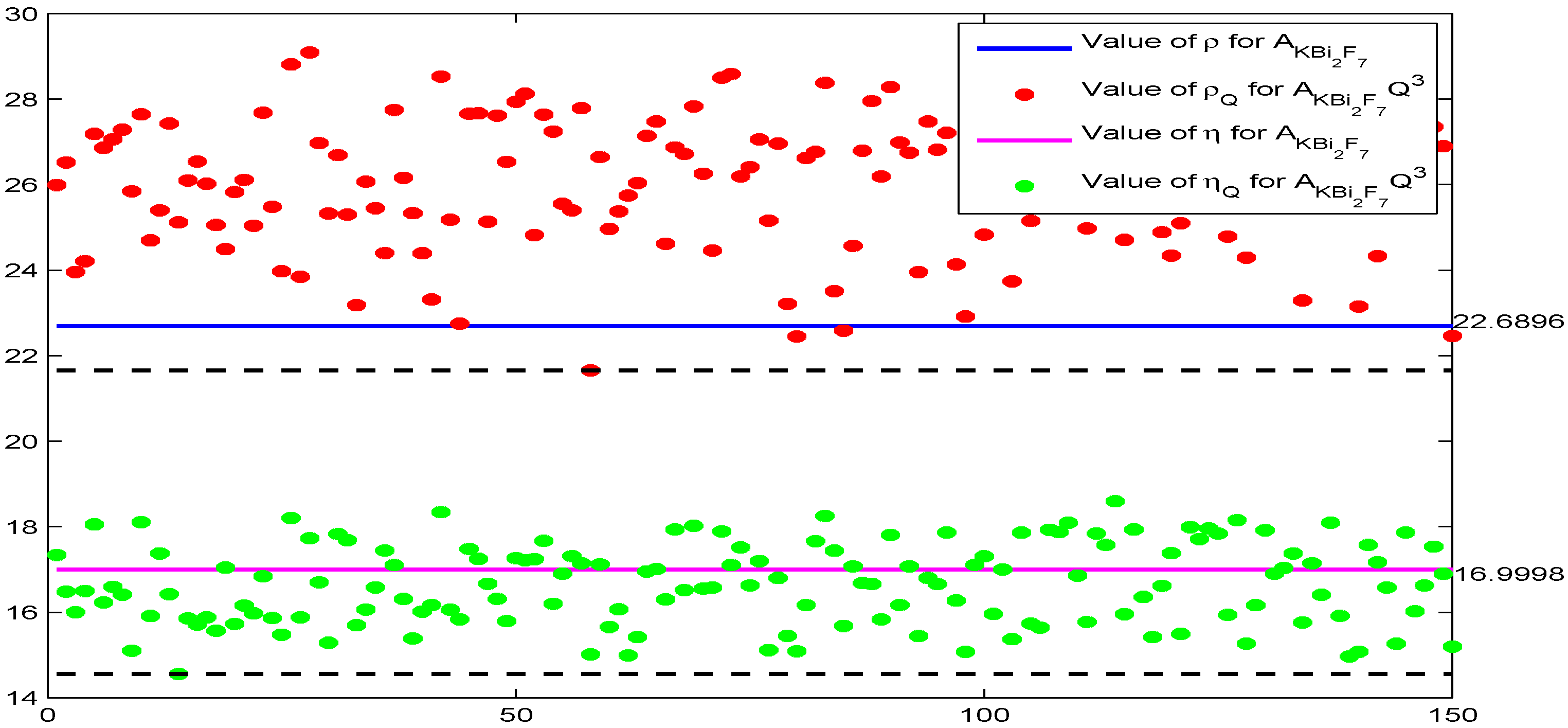
Remark 2.

It is easy to verify that

$$\begin{array}{c}\hfill {(r_i^{(1)}(\mathcal{A}))}^2=\sum _{j\in N}(\sum _{k\in N}|a_{ijk}{|)}^2\le (\sum _{j\in N}\sum _{k\in N}|a_{ijk}{|)}^2={(R_i^{(1)}(\mathcal{A}))}^2,\end{array}$$

$$\begin{array}{c}\hfill {(r_k^{(3)}(\mathcal{A}))}^2=\sum _{j\in N}(\sum _{i\in N}|a_{ijk}{|)}^2\le (\sum _{j\in N}\sum _{i\in N}|a_{ijk}{|)}^2={(R_k^{(3)}(\mathcal{A}))}^2.\end{array}$$

Hence,

$$\begin{array}{c}\hfill \underset{i,k\in N}{max}\sqrt{r_i^{(1)}(\mathcal{A})r_k^{(3)}(\mathcal{A})}\le \underset{i,k\in N}{max}\sqrt{R_i^{(1)}(\mathcal{A})R_k^{(3)}(\mathcal{A})}.\end{array}$$

Thus, the interval $[-\eta ,\eta ]$ captures all C-eigenvalues of piezoelectric tensors more precisely than the interval $[-\rho ,\rho ]$ given in [12].

Similarly, the interval $[-\eta ,\eta ]$ given in Theorem 2 may not be invariant under orthogonal transformation. Following the generation process of the orthogonal matrix of Corollary 2, we obtain various values of $\rho$ and ${\rho }_Q$ in [12] and $\eta$ and ${\eta }_Q$ for ${\mathcal{A}}_{KB{i}_2{F}_7}$ and ${\mathcal{A}}_{KB{i}_2{F}_7}{Q}^3$; see Figure 2.

Figure 2. Comparisons among $\rho$ and ${\rho }_Q$ in [12] and $\eta$ and ${\eta }_Q$ for ${\mathcal{A}}_{KB{i}_2{F}_7}$ and ${\mathcal{A}}_{KB{i}_2{F}_7}{Q}^3$.

Corollary 2.

Let ${\lambda }^{*}$ be the largest C-eigenvalue of piezoelectric tensor $\mathcal{A}=(a_{ijk})\in {\mathbb{R}}^{n\times n\times n}$. Then

$$\begin{array}{c}\hfill {\lambda }^{*}\le \underset{Q\in {\mathcal{Q}}^{n\times n}}{min}{\eta }_Q\le \eta ,\end{array}$$

where ${\delta }_Q=\underset{i,k\in N}{max}\sqrt{r_i^{(1)}(\mathcal{A}{Q}^3)r_k^{(3)}(\mathcal{A}{Q}^3)}.$

In the following, we propose a sharp C-eigenvalue inclusion interval based on the symmetry of piezoelectric tensors.

Theorem 3.

Let λ be a C-eigenvalue of piezoelectric tensor $\mathcal{A}=(a_{ijk})$. Then

$$\lambda \in [-\tau ,\tau ],$$

where $\tau =\sqrt{{\displaystyle \sum _{i\in N}}(\underset{j\in N}{max}{\displaystyle \sum _{k\in N}}|a_{ijk}{|)}^2}.$

Proof. 

It follows from (ii) of Lemma 1 that

$$\begin{array}{cc}\hfill \lambda =& \hfill \{x\mathcal{A}yy:x^{\top }x=1and{y}^{\top }y=1,x,y\in {\mathbb{R}}^n\}.\hfill \end{array}$$

For C-eigenvalue $\lambda$, using Cauchy inequality, we obtain

$$\begin{array}{c}\hfill \lambda \le \underset{x,y}{max}x\mathcal{A}yy\le \underset{x,y}{max}\sqrt{\sum _{i\in N}{x}_i^2}\sqrt{\sum _{i\in N}{(\mathcal{A}yy)}_i^2}\le \underset{y}{max}\sqrt{\sum _{i\in N}(\underset{y}{max}{|(\mathcal{A}yy)}_i{|)}^2},\end{array}$$

(8)

where ${(\mathcal{A}yy)}_i={\displaystyle \sum _{j,k\in N}}{a}_{ijk}{y}_j{y}_k.$ Further,

$$\underset{y}{max}{|(\mathcal{A}yy)}_i|=\underset{y}{max}|y^{\top }\mathcal{A}(i,:,:)y|,$$

where $\mathcal{A}(i,:,:)$ is a symmetric matrix. Then, it follows from Girshgorin circles for the matrices $\mathcal{A}(i,:,:)$ that

$$\underset{y}{max}{|(\mathcal{A}yy)}_i|\le \underset{j\in N}{max}\sum _{k\in N}|a_{ijk}|,$$

which implies

$$\begin{array}{c}\hfill \lambda \le \sqrt{\sum _{i\in N}(\underset{j\in N}{max}\sum _{k\in N}|a_{ijk}{|)}^2}.\end{array}$$

□

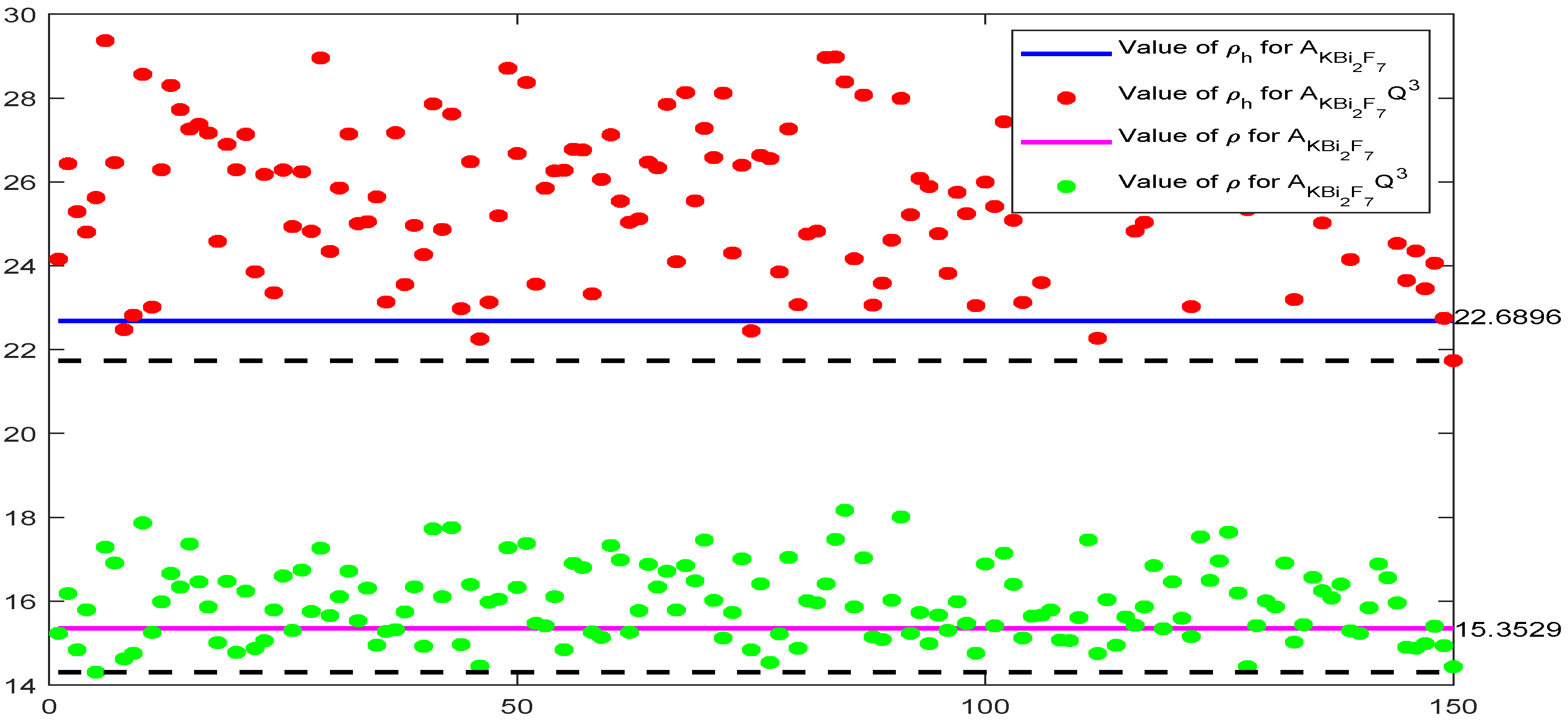
It should be noted that interval $[-\tau ,\tau ]$ given in Theorem 3 may not be invariant under orthogonal transformation. In fact, following the generation process of the orthogonal matrix of Corollary 1, we can obtain various values of $\rho$ and ${\rho }_Q$ in [12] and $\tau$ and ${\tau }_Q$ for ${\mathcal{A}}_{KB{i}_2{F}_7}$ and ${\mathcal{A}}_{KB{i}_2{F}_7}{Q}^3$; see Figure 3.

Figure 3. Comparisons among $\rho$ and ${\rho }_Q$ in [12] and $\tau$ and ${\tau }_Q$ for ${\mathcal{A}}_{KB{i}_2{F}_7}$ and ${\mathcal{A}}_{KB{i}_2{F}_7}{Q}^3$.

Corollary 3.

Let ${\lambda }^{*}$ be the largest C-eigenvalue of piezoelectric tensor $\mathcal{A}=(a_{ijk})\in {\mathbb{R}}^{n\times n\times n}$. Then

$${\lambda }^{*}\le \underset{Q\in {\mathcal{Q}}^{n\times n}}{min}{\tau }_Q\le \delta ,$$

where ${\tau }_Q=\sqrt{\sum _{i\in N}(\underset{j\in N}{max}(\sum _{k\in N}|{(\mathcal{A}{Q}^3)}_{ijk}{|))}^2}.$

Now, we utilize numerical examples given in [2,3,8,21] to show the superiority of the obtained results.

Example. 1.

(I) Take piezoelectric tensor ${\mathcal{A}}_{VFeSb}$ with its nonzero entries

$$\begin{array}{c}\hfill a_{123}=a_{213}=a_{312}=-3.68180667.\end{array}$$

(II) Take piezoelectric tensor ${\mathcal{A}}_{Si{O}_2}$ with its nonzero entries

$$\begin{array}{c}\hfill a_{111}=-a_{122}=-a_{212}=-0.13685and{a}_{123}=-a_{213}=-0.009715.\end{array}$$

(III) Take piezoelectric tensor ${\mathcal{A}}_{C{r}_{2}AgBi{O}_8}$ with its nonzero entries

$$\begin{array}{cc}\hfill & a_{123}=a_{213}=-0.22163,a_{113}=-a_{223}=2.608665,\hfill \\ \hfill & a_{311}=-a_{322}=0.152485,a_{312}=-0.37153.\hfill \end{array}$$

(IV) Take piezoelectric tensor ${\mathcal{A}}_{RbTa{O}_3}$ with its nonzero entries

$$\begin{array}{cc}\hfill & a_{113}=a_{223}=-8.40955,a_{222}=-a_{212}=-a_{211}=-5.412525,\hfill \\ \hfill & a_{311}=a_{322}=-4.3031,a_{333}=-5.14766.\hfill \end{array}$$

(V) Take piezoelectric tensor ${\mathcal{A}}_{NaBi{S}_2}$ with its nonzero entries

$$\begin{array}{cc}\hfill & a_{113}=-8.90808,a_{223}=-0.00842,a_{311}=-7.11526,\hfill \\ \hfill & a_{322}=-0.6222,a_{333}=-7.93831.\hfill \end{array}$$

(VI) Take piezoelectric tensor ${\mathcal{A}}_{LiBi{B}_2{O}_5}$ with its nonzero entries

$$\begin{array}{cc}\hfill & a_{123}=2.35682,a_{112}=0.34929,a_{211}=0.16101,a_{222}=0.12562,\hfill \\ \hfill & a_{233}=0.1361,a_{213}=-0.05587,a_{323}=6.91074,a_{312}=2.57812.\hfill \end{array}$$

(VII) Take piezoelectric tensor ${\mathcal{A}}_{KB{i}_2{F}_7}$ in the above; also see [8,21].

(VIII) Take piezoelectric tensor ${\mathcal{A}}_{BaNi{O}_3}$ with its nonzero entries

$$\begin{array}{c}\hfill a_{113}=a_{223}=0.038385,a_{311}=a_{322}=6.89822,a_{333}=27.4628.\end{array}$$

We locate all C-eigenvalues of the above eight piezoelectric tensors by different methods. Since each interval mentioned above is symmetric about the origin, we only list the right boundary of each interval. Numerical results are shown in Table 1.

Table 1. Comparisons among Li’s method [12], Che’s method [13], Xiong’s method [16], He’s method [14], Liu’s method [15] and our method.

	${\mathcal{A}}_{\mathit{V}\mathit{F}\mathit{e}\mathit{S}\mathit{b}}$	${\mathcal{A}}_{{\mathit{SiO}}_2}$	${\mathcal{A}}_{{\mathit{Cr}}_2{\mathit{AgBiO}}_8}$	${\mathcal{A}}_{\mathit{RbT}{\mathit{aO}}_3}$	${\mathcal{A}}_{{\mathit{NaBiS}}_2}$	${\mathcal{A}}_{{\mathit{LiBiB}}_2{\mathit{O}}_5}$	${\mathcal{A}}_{{\mathit{KBi}}_2{\mathit{F}}_7}$	${\mathcal{A}}_{{\mathit{BaNiO}}_3}$
${\lambda }^{*}$	$4.2514$	$0.1375$	$2.6258$	$12.4234$	$11.6674$	$7.7376$	$13.5021$	$27.4628$
$\rho$	$7.3636$	$0.2882$	$5.6606$	$30.0911$	$17.3288$	$15.2911$	$22.6896$	$38.8162$
${\rho }_{min}$	$7.3636$	$0.2834$	$5.6606$	$23.5377$	$16.8548$	$12.3206$	$20.2351$	$35.3787$
${\rho }_{\Gamma }$	$7.3636$	$0.2834$	$5.6606$	$23.5377$	$16.8548$	$12.3206$	$20.2351$	$27.5396$
${\rho }_{\mathcal{L}}$	$7.3636$	$0.2734$	$4.8058$	$23.5377$	$16.5640$	$11.0127$	$18.8793$	$27.5109$
${\rho }_{\mathcal{M}}$	$7.3636$	$0.2834$	$4.7861$	$23.5377$	$16.8464$	$11.0038$	$19.8830$	$27.5013$
${\rho }_{{\rm Y}}$	$7.3636$	$0.2834$	$4.7335$	$23.5377$	$16.8464$	$10.9998$	$19.8319$	$27.5013$
${\rho }_{{\Omega }^S}$	$7.3636$	$0.2738$	$4.2732$	$23.0353$	$16.8464$	$10.2581$	$17.7874$	$27.4629$
${\tilde{\rho }}_{min}$	$7.3636$	$0.2393$	$4.6717$	$22.7163$	$14.5723$	$12.1694$	$18.7025$	$27.5396$
$\delta$	$5.2068$	$0.2038$	$4.0026$	$21.2776$	$12.2533$	$10.8123$	$18.2321$	$27.5011$
$\eta$	$5.2068$	$0.1934$	$3.9284$	$18.1473$	$12.2221$	$10.8081$	$16.9998$	$28.2909$
$\tau$	$6.3371$	$0.2073$	$4.0373$	$16.9703$	$11.8319$	$9.1696$	$15.3529$	$27.4629$

In Table 1, ${\lambda }^{*}$ represents the largest C-eigenvalue of a piezoelectric tensor; $\rho$ and ${\rho }_{min}$ are the right boundaries of the intervals $[-\rho ,\rho ]$ and $[-{\rho }_{min},{\rho }_{min}]$ obtained by Theorems 1 and 2 of [12]; ${\tilde{\rho }}_{min}$ is the right boundary of the interval $[-{\tilde{\rho }}_{min},{\tilde{\rho }}_{min}]$ obtained by Theorem 2.1 of [15]; ${\rho }_{\Gamma },{\rho }_{\mathcal{L}}$ and ${\rho }_{\mathcal{M}}$ are the right boundaries of the intervals $[-{\rho }_{\Gamma },{\rho }_{\Gamma }],[-{\rho }_{\mathcal{L}},{\rho }_{\mathcal{L}}]$ and $[-{\rho }_{\mathcal{M}},{\rho }_{\mathcal{M}}]$ obtained by Theorems 2.1, 2.2 and 2.4 of [13]; ${\rho }_{{\rm Y}}$ is the right boundary of the interval $[-{\rho }_{{\rm Y}},{\rho }_{{\rm Y}}]$ obtained by Theorem 2.1 of [16]; ${\rho }_{{\Omega }^S}$ is the right boundary of the interval $[-{\rho }_{{\Omega }^S},{\rho }_{{\Omega }^S}]$ obtained by Theorem 5 of [14]; $\delta ,\eta$ and $\tau$ are the right boundaries of the intervals $[-\delta ,\delta ],[-\eta ,\eta ]$ and $[-\tau ,\tau ]$ obtained by Theorems 1–3. Numerical results reveal that our results are sharper than those of [12,13,14,15,16] Table 1.

3. Efficiency Evaluation of the Best Rank-One Approximation of Piezoelectric Tensors

In this section, we will propose sharp bound estimations of the largest C-eigenvalue, and evaluate the efficiency of the best rank-one approximation of piezoelectric tensors based on the quotient of the residual $\omega$ in [22,23,24]. First, we give a lower bound of the largest C-eigenvalue for the piezoelectric tensor $\mathcal{A}$.

Theorem 4.

Let ${\lambda }^{*}$ be the largest C-eigenvalue of piezoelectric tensor $\mathcal{A}=(a_{ijk})\in {\mathbb{R}}^{n\times n\times n}$. Then,

$$\begin{array}{c}\hfill {\lambda }^{*}\ge max\left\{\underset{i,j\in N}{max}|a_{ijj}|,\frac{|{\displaystyle \sum _{i,j,k\in N}}{a}_{ijk}|}{n\sqrt{n}}\right\}=\kappa .\end{array}$$

Proof. 

It follows from (iii) of Lemma 1 that

$$\begin{array}{c}\hfill {\lambda }^{*}=max\{x\mathcal{A}yy:x^{\top }x=1,y^{\top }y=1,x,y\in {\mathbb{R}}^n\}.\end{array}$$

(9)

Next, we break down the proof into two cases to show ${\lambda }^{*}\ge \underset{i,j\in N}{max}|a_{ijj}|.$

Case I. $a_{ijj}\ge 0.$ Set

$$(\tilde{x},\tilde{y})=\left\{\begin{array}{c}\hfill x_i=1,y_j=1;\hfill \\ \hfill 0,otherwise.\hfill \end{array}\right.$$

By (9), it holds that

$$\begin{array}{c}\hfill {\lambda }^{*}\ge \tilde{x}\mathcal{A}\tilde{y}\tilde{y}=a_{ijj}.\end{array}$$

(10)

Case II. $a_{ijj}<0.$ Set

$$(\tilde{x},\tilde{y})=\left\{\begin{array}{c}\hfill x_i=-1,y_j=1;\hfill \\ \hfill 0,otherwise.\hfill \end{array}\right.$$

It follows from (9) that

$${\lambda }^{*}\ge \tilde{x}\mathcal{A}\tilde{y}\tilde{y}=-a_{ijj}.$$

Summing up the above two cases, one has

$$\begin{array}{c}\hfill {\lambda }^{*}\ge \underset{i,j\in N}{max}|a_{ijj}|.\end{array}$$

(11)

In order to prove ${\lambda }^{*}\ge \frac{|{\displaystyle \sum _{i,j,k\in N}}{a}_{ijk}|}{n\sqrt{n}}$, we set

$$(\tilde{x},\tilde{y})=\left\{\begin{array}{c}{x}_i=\frac{1}{\sqrt{n}},y_j=\frac{1}{\sqrt{n}},y_k=\frac{1}{\sqrt{n}},j,k\in N,j\ne k;\hfill \\ 0,otherwise;\hfill \end{array}\right.$$

or

$$(\tilde{x},\tilde{y})=\left\{\begin{array}{c}{x}_i=-\frac{1}{\sqrt{n}},y_j=\frac{1}{\sqrt{n}},y_k=\frac{1}{\sqrt{n}},j,k\in N,j\ne k;\hfill \\ 0,otherwise.\hfill \end{array}\right.$$

Following similar arguments to the proof of Cases I and II, we obtain

$$\begin{array}{c}\hfill {\lambda }^{*}\ge \frac{|{\displaystyle \sum _{i,j,k\in N}}{a}_{ijk}|}{n\sqrt{n}}.\end{array}$$

(12)

It follows from (11) and (12) that

$$\begin{array}{c}\hfill {\lambda }^{*}\ge max\left\{\underset{i,j\in N}{max}|a_{ijj}|,\frac{|{\displaystyle \sum _{i,j,k\in N}}{a}_{ijk}|}{n\sqrt{n}}\right\}=\kappa .\end{array}$$

□

In what follows, we propose lower bounds of the largest C-eigenvalue of the eight piezoelectric tensors in Example 1. Numerical results are shown in Table 2, where $\kappa$ represents the lower bound of the largest C-eigenvalue for a piezoelectric tensor.

Table 2. Lower bound estimations of the largest C-eigenvalue in Theorem 4.

	${\mathcal{A}}_{\mathit{VFeSb}}$	${\mathcal{A}}_{{\mathit{SiO}}_2}$	${\mathcal{A}}_{{\mathit{Cr}}_2{\mathit{AgBiO}}_8}$	${\mathcal{A}}_{\mathit{RbT}{\mathit{aO}}_3}$	${\mathcal{A}}_{{\mathit{NaBiS}}_2}$	${\mathcal{A}}_{{\mathit{LiBiB}}_2{\mathit{O}}_5}$	${\mathcal{A}}_{{\mathit{KBi}}_2{\mathit{F}}_7}$	${\mathcal{A}}_{{\mathit{BaNiO}}_3}$
${\lambda }^{*}$	$4.2514$	$0.1375$	$2.6258$	$12.4234$	$11.6674$	$7.7376$	$13.5021$	$27.4628$
$\kappa$	$4.2514$	$0.1369$	$0.1525$	$7.9661$	$7.9383$	$4.7538$	$12.6439$	$27.4628$

In the following, we propose bound estimations for the quotient of the residual $\omega$, which evaluate the efficiency of the best rank-one approximation for piezoelectric tensors.

Theorem 5.

For piezoelectric tensor $\mathcal{A}=(a_{ijk})\in {\mathbb{R}}^{n\times n\times n}$, it holds that

$$\begin{array}{c}\hfill \frac{\sqrt{{||\mathcal{A}||}_F^2-{\kappa }^2}}{{||\mathcal{A}||}_F}\ge \omega \ge max\left\{\frac{\sqrt{{||\mathcal{A}||}_F^2-{\delta }^2}}{{||\mathcal{A}||}_F},\frac{\sqrt{{||\mathcal{A}||}_F^2-{\eta }^2}}{{||\mathcal{A}||}_F},\frac{\sqrt{{||\mathcal{A}||}_F^2-{\tau }^2}}{{||\mathcal{A}||}_F}\right\},\end{array}$$

where $\delta ,\tau ,\eta$ and κ are defined in Theorems 1–4.

Proof. 

Since $\mathcal{A}$ is a piezoelectric tensor, from Lemma 2, we deduce that ${\lambda }^{*}{x}^{*}\circ y^{*}\circ y^{*}$ is a best rank-one approximation of $\mathcal{A}$, i.e.,

$$\begin{array}{c}\hfill \underset{\lambda ,x,y}{min}||\mathcal{A}-\lambda x\circ y\circ {y||}_F^2=||\mathcal{A}-{\lambda }^{*}{x}^{*}\circ y^{*}\circ y^{*}{||}_F^2={||\mathcal{A}||}_F^2-{{\lambda }^{*}}^2,\end{array}$$

where ${\lambda }^{*}$ is the largest C-eigenvalue. From Theorems 1–4, we obtain that the quotient of the residual of piezoelectric tensor $\mathcal{A}$ is

$$\begin{array}{cc}\hfill \frac{\sqrt{{||\mathcal{A}||}_F^2-{\kappa }^2}}{{||\mathcal{A}||}_F}& \ge \omega =\frac{||\mathcal{A}-{\lambda }^{*}{x}^{*}\circ y^{*}\circ y^{*}{||}_F}{{||\mathcal{A}||}_F}=\sqrt{1-\frac{{{\lambda }^{*}}^2}{{||\mathcal{A}||}_F^2}}\hfill \\ \hfill & \ge max\left\{\frac{\sqrt{{||\mathcal{A}||}_F^2-{\delta }^2}}{{||\mathcal{A}||}_F},\frac{\sqrt{{||\mathcal{A}||}_F^2-{\eta }^2}}{{||\mathcal{A}||}_F},\frac{\sqrt{{||\mathcal{A}||}_F^2-{\tau }^2}}{{||\mathcal{A}||}_F}\right\}.\hfill \end{array}$$

□

In the following, we will calculate the quotient of the residual $\omega$ of the eight piezoelectric tensors in Example 1. For the first piezoelectric tensor ${\mathcal{A}}_{VFeSb},$ we know $4.2514\le {\lambda }^{*}\le 5.2068$ from Table 1 and Table 2, where ${\lambda }^{*}$ represents the largest C-eigenvalue. Thus, we compute

$$0.8165\le \omega =\frac{||\mathcal{A}-{\lambda }^{*}\overline{x}\circ \overline{y}\circ \overline{y}{||}_F}{{||\mathcal{A}||}_F}\le 0.8819,$$

which evaluates the efficiency of the best rank-one approximation for piezoelectric tensor ${\mathcal{A}}_{VFeSb}.$ The quotients of the residual $\omega$ of the other seven piezoelectric tensors in Example 1 are listed in Table 3.

Table 3. Bound estimations of the quotient for the residual $\omega$.

	${\mathcal{A}}_{VFeSb}$	${\mathcal{A}}_{Si{O}_2}$	${\mathcal{A}}_{C{r}_{2}AgBi{\mathit{O}}_8}$	${\mathcal{A}}_{RbTa{O}_3}$
$\omega$	$[0.8165,0.8819]$	$[0.7094,0.8264]$	$[0.8450,0.9996]$	$[0.6155,0.9290]$
	${\mathcal{A}}_{NaBi{S}_2}$	${\mathcal{A}}_{LiBi{B}_2{O}_5}$	${\mathcal{A}}_{KB{i}_2{F}_7}$	${\mathcal{A}}_{BaNi{O}_3}$
$\omega$	$[0.6915,0.8211]$	$[0.4857,0.9011]$	$[0.1142,0.4286]$	$[0.3346,0.3347]$

4. Conclusions

In this paper, we proposed sharp C-eigenvalue inclusion intervals based on the structure of piezoelectric tensors and obtained good numerical results. More importantly, we established not only the upper bound but also the lower bound of the largest C-eigenvalues to evaluate the efficiency of the best rank-one approximation of piezoelectric tensors. It is unfortunate that we attempted to estimate the largest C eigenvalue but did not obtain the real largest C-eigenvalue. Further studies can be considered to develop efficient algorithms to calculate quickly the largest C-eigenvalue of a high-dimensional piezoelectric tensor by our C-eigenvalue inclusion intervals.