An Earthquake-Clustering Model in North Aegean Area (Greece)

Abstract

The investigation of short-term earthquake-clustering features is made feasible through the application of a purely stochastic Epidemic-Type Aftershock Sequence (ETAS) model. The learning period that is used for the estimation of the parameters is composed by earthquakes with M ≥ 2.6 that occurred between January 2008 and May 2017. The model predictability is retrospectively examined for the 12 June 2017 Lesvos earthquake (M_w6.4) and the subsequent events. The construction of time-dependent seismicity maps and comparison between the observed and expected earthquake number are performed in order to temporally and spatially test the evolution of the sequence, respectively. The generation of 127 target events with M ≥ 3.0 in the period June–July 2017, just before the main shock occurrence, is examined in a quantitative evaluation. The statistical criteria used for assessing the model performance are the Relative Operating Characteristic Diagram, the R-score, and the probability gain. Reliable forecasts are provided through the epidemic model testifying its superiority towards a time-invariant Poisson model.

1. Introduction

It is widely accepted that a large earthquake is followed by an increased seismicity rate for several years [1] and at distinctly larger distances—2 or 3 times—than its rupture length [2,3,4]. The investigation of clustering features of seismicity both in time and space has proved to be one of the most important elements of earthquake forecasting in recent decades. From a statistical point of view, the Epidemic-Type Aftershock Sequence (ETAS) model [5,6,7,8] became the most popular in the scientific community and is introduced as the most suitable model for describing the short-term seismicity [9,10].

During the evolution of a seismic sequence, when the magnitude of an earthquake is smaller than that of the previous one, the event is considered an aftershock. This definition is rather arbitrary and the distinction between “foreshocks”, “main shocks” and “aftershocks” is not a trivial procedure. The concept upon which the epidemic models are developed is that there is no need to distinguish this earthquake property. Each event above the magnitude threshold, irrespective of whether it is small or large, is regarded as being able to generate its own descendants. None of them is independent but rather related to the previous events according to certain criteria and upon a certain weight. Since its development, the ETAS model and its extensions have been widely applied towards operational earthquake forecasting, particularly following a large earthquake [11,12,13,14]. Reliable forecasts for main shocks have also been demonstrated through ETAS models [15,16,17,18].

The validation of earthquake-forecasting models constitutes an important component of the application. This is the main concept behind international cooperation such as the Collaboratory for the Study of Earthquake Predictability (CSEP) [19]. The conducted tests assess the performance of the models and aim at quantitatively specifying the uncertainties involved in earthquake forecasts. These forecasts are computed in statistical terms towards the probabilistic hazard assessment of earthquake risk [20,21,22].

The model application in the northern Aegean Sea is considered both suitable and necessary, given that the study area attracts high seismological interest since it undergoes intense active deformation, producing increased seismicity rates and frequent occurrences of strong (M ≥ 6.0) earthquakes. Strong (M ≥ 6.0) earthquakes are frequently recorded in both the historical and instrumental eras, and in particular seven main shocks of M ≥ 6.0 have occurred since 1980. These strong earthquakes along with the intense seismic activity of smaller events offer a unique opportunity to apply and test clustering models and track the evolution of the forthcoming sequences. Aiming to retrospectively test its short-term predictability efficiency, the epidemic model by Console & Murru [7] is applied to earthquakes that occurred in the area since January 2008. Particularly, the occurrence of the 12 June 2017, M_w6.4 earthquake located south of Lesvos Island along with its aftershock sequence are under investigation to corroborate and examine the model’s performance. The evaluation of this performance is carried out through statistical methods based on a binary approach, notably, the Relative Operating Characteristics (ROC) diagrams, the R-score and the probability gain.

2. Brief Description of the Earthquake-Clustering Model

The model considers earthquakes as the realization of a Hawkes process, namely as a point with coordinates (x, y, t, m) corresponding to its geographical position (x, y), occurrence time (t) and earthquake magnitude (m). As in previous publications [7,8,23], we neglected depth as a spatial coordinate. We based this decision on the fact that the depths of the crustal earthquakes in our catalog range between 3 and 15 km. This consideration reduces the involved location errors, which are higher for depth estimation in comparison with the horizontal coordinate’s estimation. The basic assumption of the epidemic model is that each event is triggered by the previous events and is capable of triggering subsequent events depending upon its magnitude and spatial and temporal distance from the other events.

The expected occurrence-rate density, λ, for earthquakes with magnitudes above a threshold, is modeled as the superposition of spontaneous and triggered events, as

$$\lambda \left(x,y,t,m\right)=f_r{\lambda }_0\left(x,y,m\right)+{\displaystyle \sum }_{i=1}^{N}H\left(t-t_i\right){\lambda }_i\left(x,y,t,m\right)$$

(1)

where $f_r$ is a factor called “failure rate” that constitutes a measure of the fraction of independent earthquakes with reference to the total number of earthquakes and represents the spontaneous background seismicity, ${\lambda }_0\left(x,y,m\right)$ is the total time-invariant background seismicity rate, $t_i$ is the occurrence time of each of the N earthquakes, H(t) is the Heaviside step function, such that $H\left(t\right)=0$ for $t\le 0$ and $H\left(t\right)=1$ for $t>0$, and ${\lambda }_i\left(x,y,t,m\right)$ is the kernel function describing the single contribution of each past event and depends on the magnitude and the spatial distance from the triggering earthquake and the time lapse between this event’s occurrence time and the target time.

The first and the second term of the right-hand side of Equation (1) represent the time-invariant background “spontaneous” and the time-varying “triggered” seismic activity, respectively. This means that any earthquake is not truly independent or dependent on any other single earthquake, but it is rather linked to all past earthquakes and the background seismicity, according to different weights.

Assuming that the Gutenberg–Richter (G–R) law holds, the long-term average seismicity ${\lambda }_o\left(x,y,m\right)$ can be expressed as:

$${\lambda }_0\left(x,y,m\right)={\mu }_0\left(x,y\right)\beta e^{-\beta \left(m-m_0\right)}$$

(2)

where ${\mu }_0\left(x,y\right)$ is the spatial density of earthquakes with magnitude $m\ge m_0$, $m_o$ is the magnitude cutoff and $\beta$ is connected to the b-value of the G–R law by the relation $\beta =b ln\left(10\right)$. The only criterion for the selection of the magnitude cutoff m_o is that it should be larger than the completeness magnitude. An algorithm for smoothing, introduced by Frankel [24] and then modified by Console et al. [25], is then applied in an attempt to obtain a continuous rate density ${\mu }_{\mathrm{o}}\left(x,y\right)$. Instead of distinguishing events in a binary way, i.e., as being independent or triggered, a probability is assigned to them as in the method adopted by Zhuang et al. [26]. The iterative adjustment of the weights is carried out in a way similar to that adopted by Marsan and Longliné [27]. It should be noted that for the estimation of the smoothed distribution of the background seismicity, it is essential to compute the correlation distance, c_d, of the earthquake epicentral distribution. It could be regarded as an indicator of the spatial variability of seismicity, revealing the spatial interrelation of earthquakes.

The contribution of any past earthquake $\left(x_i,y_i,m_i,t_i\right)$ to the occurrence-rate density, λ_i, of the triggering earthquakes is expressed by three terms related to the time, magnitude and space distribution, respectively, for t > t_i,

$${\lambda }_i\left(x,y,t,m\right)=Kh\left(t-t_i\right)\beta e^{-\beta \left(m-m_i\right)}f\left(x-x_i,y-y_i\right)$$

(3)

where K is the productivity coefficient, $h\left(t\right)$ is the time and $f\left(x,y\right)$ is the space distribution.

The time dependence is given by the modified Omori law [28], according to the relation

$$h\left(t\right)=\left(p-1\right)c^{p-1}{\left(t-c\right)}^{-p}, p>1,$$

(4)

where c and p are characteristic parameters of the process.

The spatial distribution is modeled through a function $f\left(x-x_i,y-y_i\right)$ with circular symmetry around the point with coordinates $\left(x_i, y_i\right)$, which is the location of the earthquake with magnitude m_i. In polar coordinates (r, θ), the function can be written as

$$f\left(r, \theta \right)=\frac{\left(q-1\right)}{\pi }\frac{d^{2\left(q-1\right)}}{{\left(r^2+d^2\right)}^q}$$

(5)

where r is the distance of $\left(x, y\right)$ from $\left(x_i, y_i\right)$, q is a free parameter, $d=d_0{e}^{\alpha \left(m_i-m_0\right)}$ with d₀ being the characteristic triggering distance for an earthquake with magnitude m_i in the spatial distribution, and α is a free parameter, the productivity parameter. This means that the average triggering distance of the aftershock zone is proportional to the square root of the main shock rupture area [29]. It is worth mentioning that the spatial function varies among different publications [26,30,31,32,33,34].

A maximum-likelihood procedure is followed for the estimation of the parameters K, $d_0$, q, α, c and p. The fraction of the spontaneous events, f_r, is not a free parameter but it depends on the other parameters since it is constrained by the condition that when Equation (1) is integrated over a very long time, it provides the total number of expected earthquakes, which is equal to the integral of λ_o(x, y, m). The β-value is independently estimated from the other parameters by means of the likelihood-estimation method of Aki [35].

3. Validation Methods

A crucial step in the application of an earthquake-forecasting model (EFM) is the validation of the results. The assessment must be performed by means of robust and rigorous tests that measure the effectiveness of the algorithm [36]. The statistical techniques employed for this purpose and carried out in this study include the Relative Operating Characteristic (ROC) diagrams, the R-score and the probability gain. Kossobokov [37], Chen et al. [38], Zechar and Jordan [39], Murru et al. [15], and Console et al. [16], among others, applied these techniques for the evaluation of earthquake-prediction algorithms and showed that the clustering epidemic model performs up to several hundred times better than a simple random forecasting hypothesis.

Although the model provides forecasts rather than predictions, these statistical methods are based on a binary approach. The whole space–time volume is divided into cells. Then, after setting a certain occurrence-rate threshold, we examined whether or not a forecast is produced and whether or not an earthquake occurred. The outcomes are summarized in a 2 × 2 contingency table where a is the number of successful forecasts of occurrence, b is the number of false alarms, c is the number of successful forecasts of non-occurrence and d is the number of events that failed to be predicted (

Table 1. Contingency table representation.

	Observed
Forecasted	Yes	No
Yes	a	b
No	d	c

).

Holliday et al. [40] proposed the terms hit rate ($H$) and false-alarm rate ($F$), estimated by the ratios $H=a/\left(a+d\right)$ and $F=b/\left(b+c\right)$. H represents the fraction of events that occurred in an alarm cell, based on a predefined threshold r and the fraction of false alarms F, i.e., events that are predicted by the model based on the probability threshold, but they have not actually occurred. When H is greater than F, the forecasting method is considered successful, while if H is equal to F the predictions are purely random. For every probability threshold, a single ROC diagram is built. The occurrence-rate threshold, r, is chosen intuitively. The smaller the value of r, the more common it is for an earthquake to be predicted by the model; yet, the number of false alarms increases.

A test statistic called R-score [41,42] is built based on the contingency table, according to the equation:

$$R=\frac{a}{a+b}-\frac{d}{c+d}$$

(6)

The values of R vary between −1 and 1. When R is equal to 1, it is assumed that all predictions, positive and negative ones, are correct, while R equal to −1 means that all the predictions are wrong, and R = 0 corresponds to random predictions. Shi et al. [43] proposed an alternative expression for the R-score with a similar interpretation:

$$R^{\prime }=\frac{a}{a+d}-\frac{b}{b+c}$$

(7)

The probability gain G is also considered as a measure of the effectiveness of the model predictability. This quantity defined by Aki [44] represents the ratio between the success rate and the average occurrence rate:

$$G=(a/\left(a+d\right))·e/\left(a+b\right)=H·e/\left(a+b\right)$$

(8)

where $e=a+b+c+d$ is the total number of cells multiplied by the number of time bins. The values of G range between 0 and ∞. When G tends to ∞, all predictions are correct, G = 1 corresponds to random predictions (similar to R = 0) and G = 0 means that all predictions are wrong.

We accomplished an additional quantitative test for a branching model’s performance by means of the branching ratio, ρ, which is defined as the average number of direct descendants generated per parent event [45,46]. In the ETAS model, the parent events are supposed to be the background events and their descendants are aftershocks, which are spatially and temporally related to the parent. Following Console et al. [47], the branching ratio is:

$$\rho =\frac{K\beta }{\beta -a}=\frac{Kbln10}{bln10-a}$$

(9)

This concept is related to the stability of a branching model. When ρ < 1 each earthquake is assumed to trigger less than one aftershock, the seismicity diminishes, and eventually the family dies. That means the process is stable and stationary, indicating that the estimated model parameters are rational [48]. On the contrary, a value of ρ > 1 means that the process generates more than one primary aftershock per earthquake, indicating that seismic activity exponentially increases with time. If we allow the ETAS parameters to change over time, the process could be occasionally explosive in a specific aftershock sequence, returning back to stability later on.

4. Study Area and Data

The study area is very frequently visited by large (M > 6.5) earthquakes, as historical information and instrumental recordings testify, most of them being associated with dextral strike–slip faulting and a NE–SW orientation, which is the dominant regional stress regime. It constitutes the northern part of the Aegean microplate, bounded in the north by the North Aegean Trough (NAT), which consists of the prolongation of the North Anatolian Fault (NAF) into the Aegean [49]. Parallel to the NAT, other parallel fault branches are running, which also accommodate large (up to M7.2) dextral strike–slip faulting earthquakes. Their conjugate counterparts, of sinistral strike–slip motion, are mainly located in the western part of the northern Aegean area, positioned almost parallel to the coastline of the Greek mainland with a NW–SE strike. Trans-tensional faulting is also present in the study area, manifested by the occurrence of M > 6.0 earthquakes that are mostly located in the eastern part of the study area. The slight diversity in the type of faulting can be dynamically interpreted as the result of the different orientations of the major regional faults with respect to the fast (~3.5 cm/yr), almost N–S extension of the back arc Aegean region due to the rollback of the eastern Mediterranean oceanic slab [50] that is subducted under the continental Aegean microplate [51].

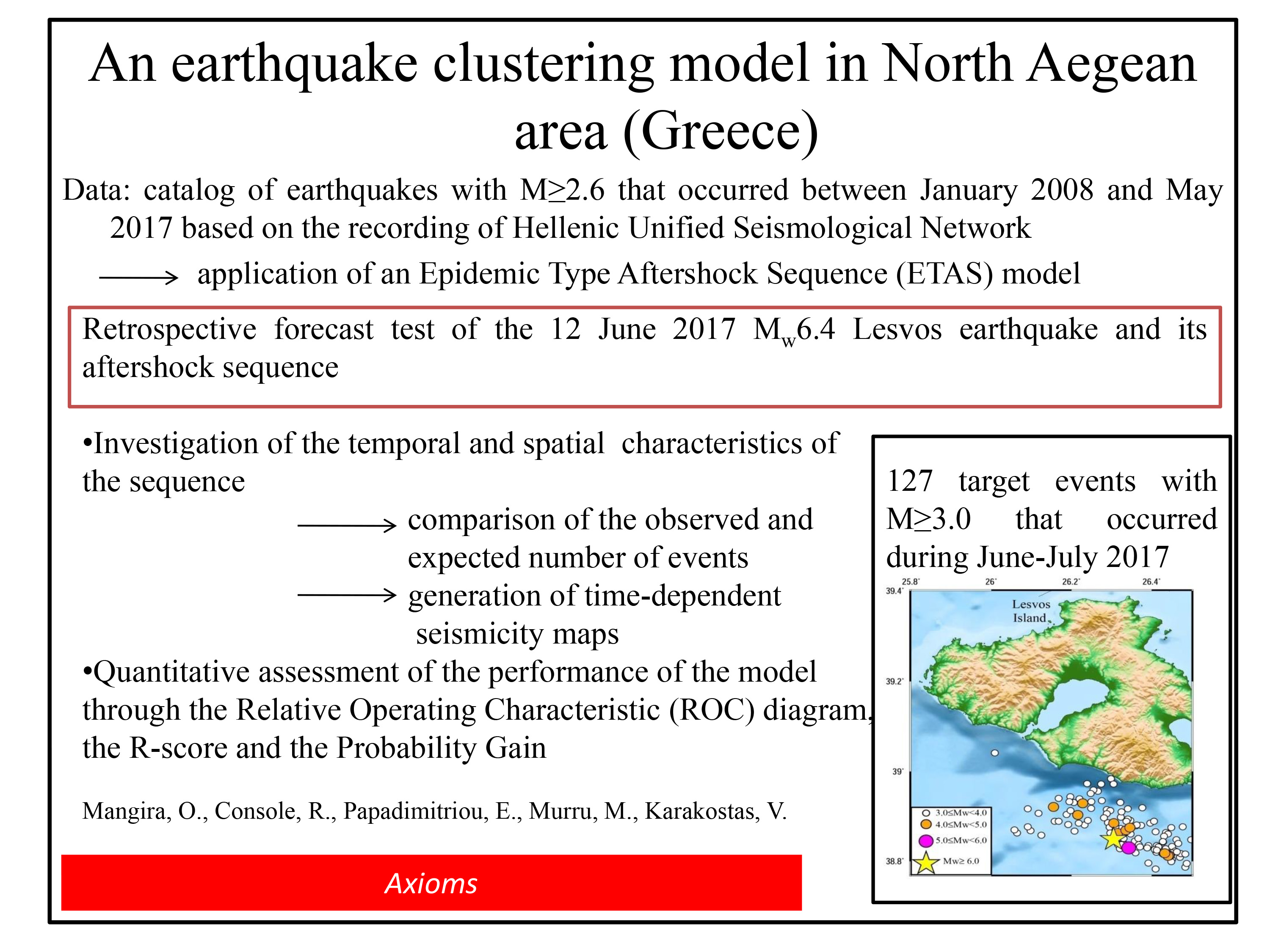
Figure 1 depicts the epicentral distribution of earthquakes with M ≥ 2.6 that occurred in the study area between January 2008 and December 2018. Seismicity is mainly concentrated along the North Aegean Trough (NAT) and onto the well-defined subparallel branches, as well as in the southeastern part where it is more diffused.

Among the most recent strong earthquakes is the 24 May 2014 M_w6.9 main shock, which occurred approximately 20 km southeast of Samothraki Island in North Aegean Trough (lat. 40.286$°$, lon. 25.375$°$). The absence of strong aftershocks with M > 5.0 as well as aftershocks very close to the main shock are two of its main characteristics [52,53]. This aftershock sequence belongs to the testing period in our analysis, as we will show in a later section.

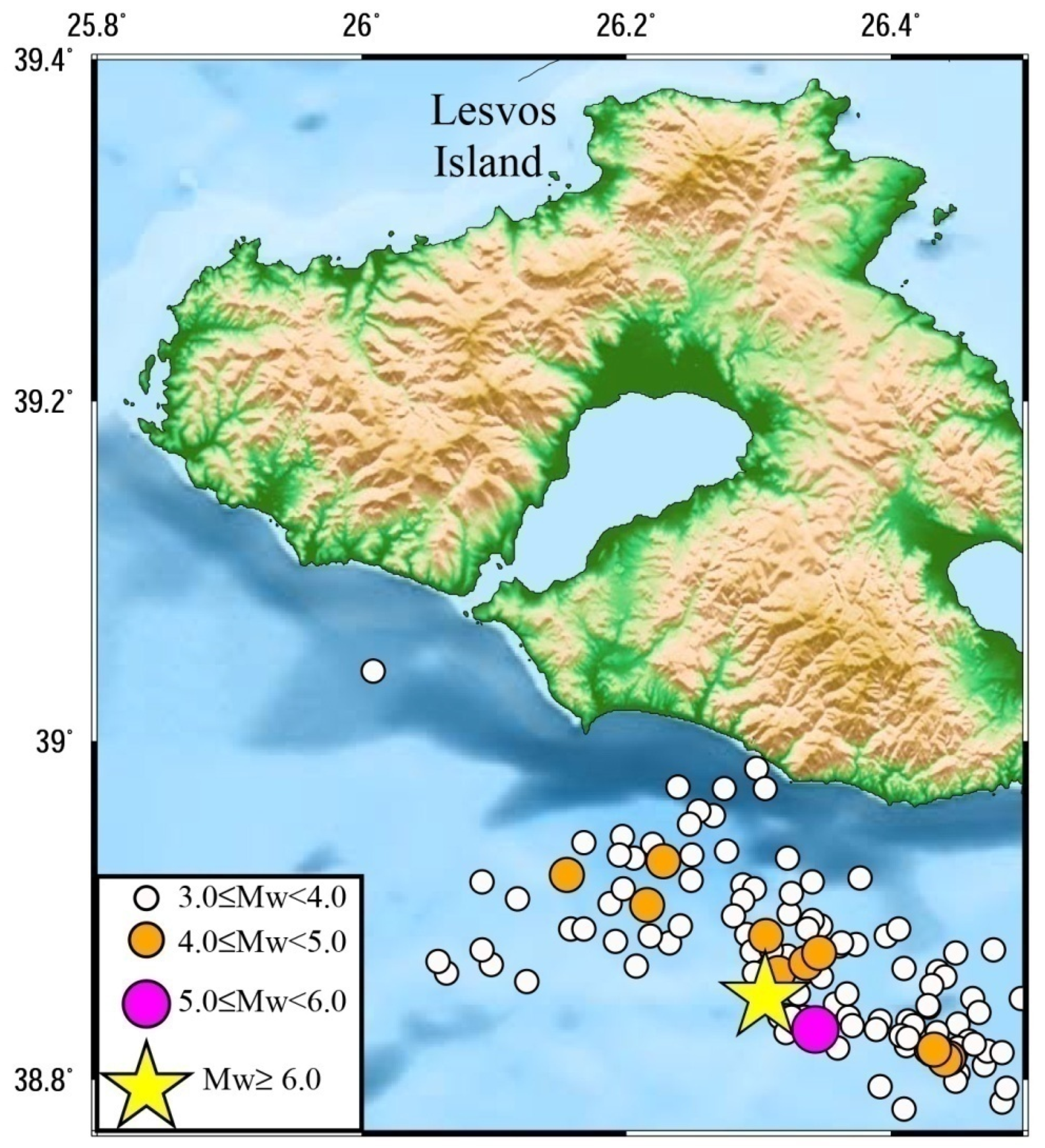
The last strong event (M_w6.4) occurred almost 15 km offshore of the southeastern coast of Lesvos Island (lat. 38.849$°$, lon. 26.305$°$) on 12 June 2017. This destructive earthquake caused one fatality, 15 injuries and extensive structural deterioration in the towns and villages of Lesvos Island. The aftershock epicentral distribution defines a NW–SE trending seismic zone offshore of the southeastern coasts of Lesvos Island. The 20 km-long seismogenic fault agrees with the seismicity spatiotemporal distribution. A vivid subsequence began with the largest aftershock (M_w5.3) on 17 June, clustering in the easternmost portion of the activated area [54]. When strong aftershocks produce secondary aftershocks within an aftershock sequence, the modified Omori law is not efficient at adequately fitting the aftershock activity. On the contrary, this fact constitutes the ETAS model suitability for the statistical analysis of the seismicity, since the fluctuation of the seismic activity is anticipated and predicted by the model. The aftershock sequence belongs to the testing period of the epidemic model.

The data used for the current study were taken from the catalog compiled by the Geophysics Department of the Aristotle University of Thessaloniki (GD–AUTh, https://doi.org/doi:10.7914/SN/HT (accessed on 1 January 2021)) [55] based on the recordings of the Hellenic Unified Seismological Network (HUSN). It is recognized that the more recent catalogs are characterized by higher quality and adequacy. In addition, it is necessary that the test of the forecasting hypothesis is carried out by means of a completely different dataset, completely independent from the one used for the formulation hypothesis. This requirement could pose a problem if the target events are large earthquakes since their recurrence times are long. In any case, the learning period should include at least one strong main shock since, in general, the learning period, as its name indicates, serves as a guide, used for estimating the parameters. The model adjusted itself to the data, and then we examined its performance using the data belonging to the testing period.

For the aforementioned reasons, the learning period was chosen to last from the 1 January of 2008 until the 31 May 2017. It includes the 2014 M_w6.9 main shock along with the swarm that occurred near the Aegean coast of northwestern Turkey during January–March 2017, which was relocated and detailed by Mesimeri et al. [56]. The completeness magnitude was equal to M_c = 2.6 according to the goodness-of-fit method (GFT) [57]. The maximum-likelihood method proposed by Aki [35] was used for the calculation of the b-value, being equal to 1.0100 ± 0.0003. The standard deviation estimate was carried out through the methodology introduced by Shi & Bolt [58]. As a result, 3919 events were included in the dataset above the magnitude threshold.

5. Results

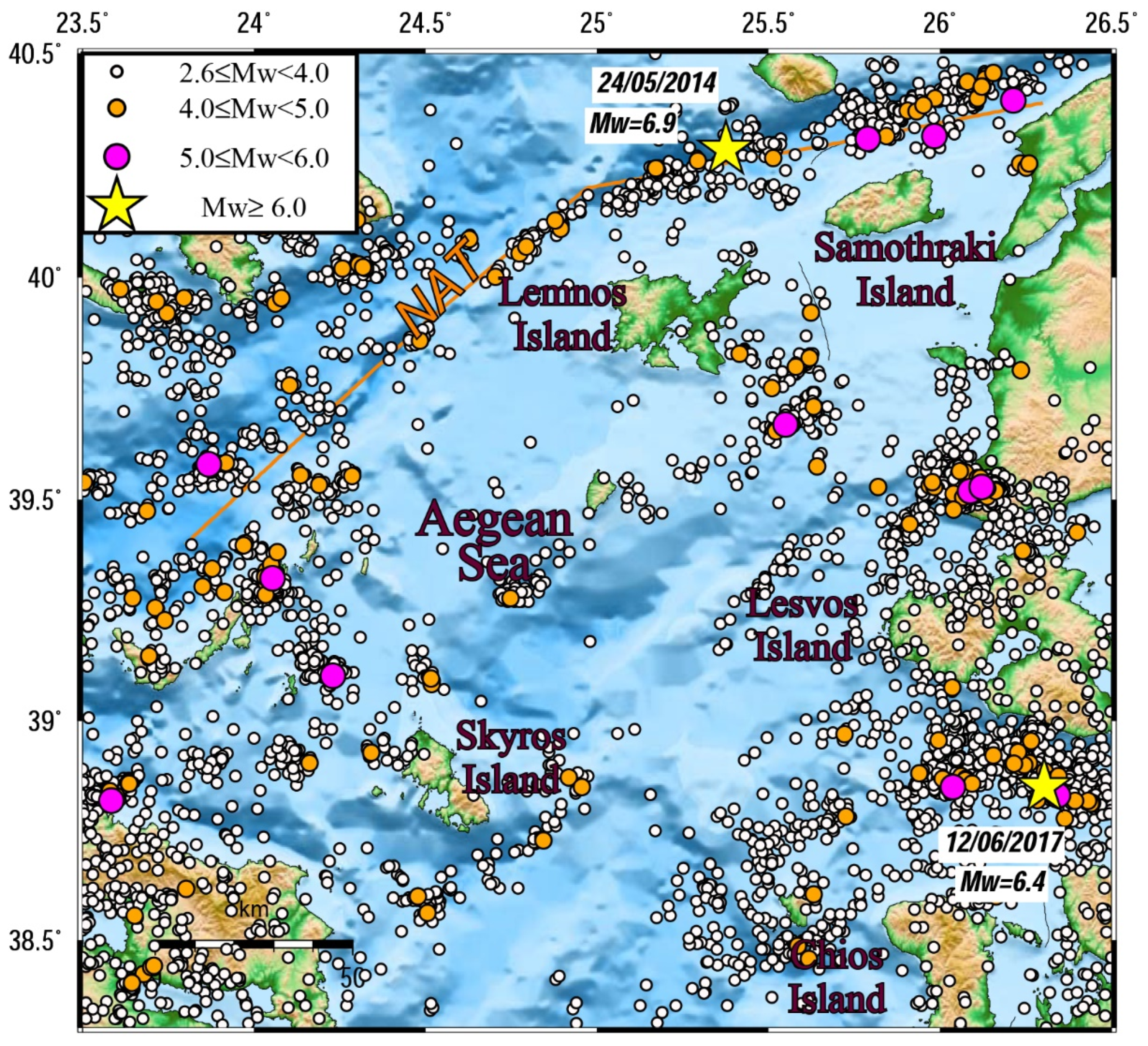
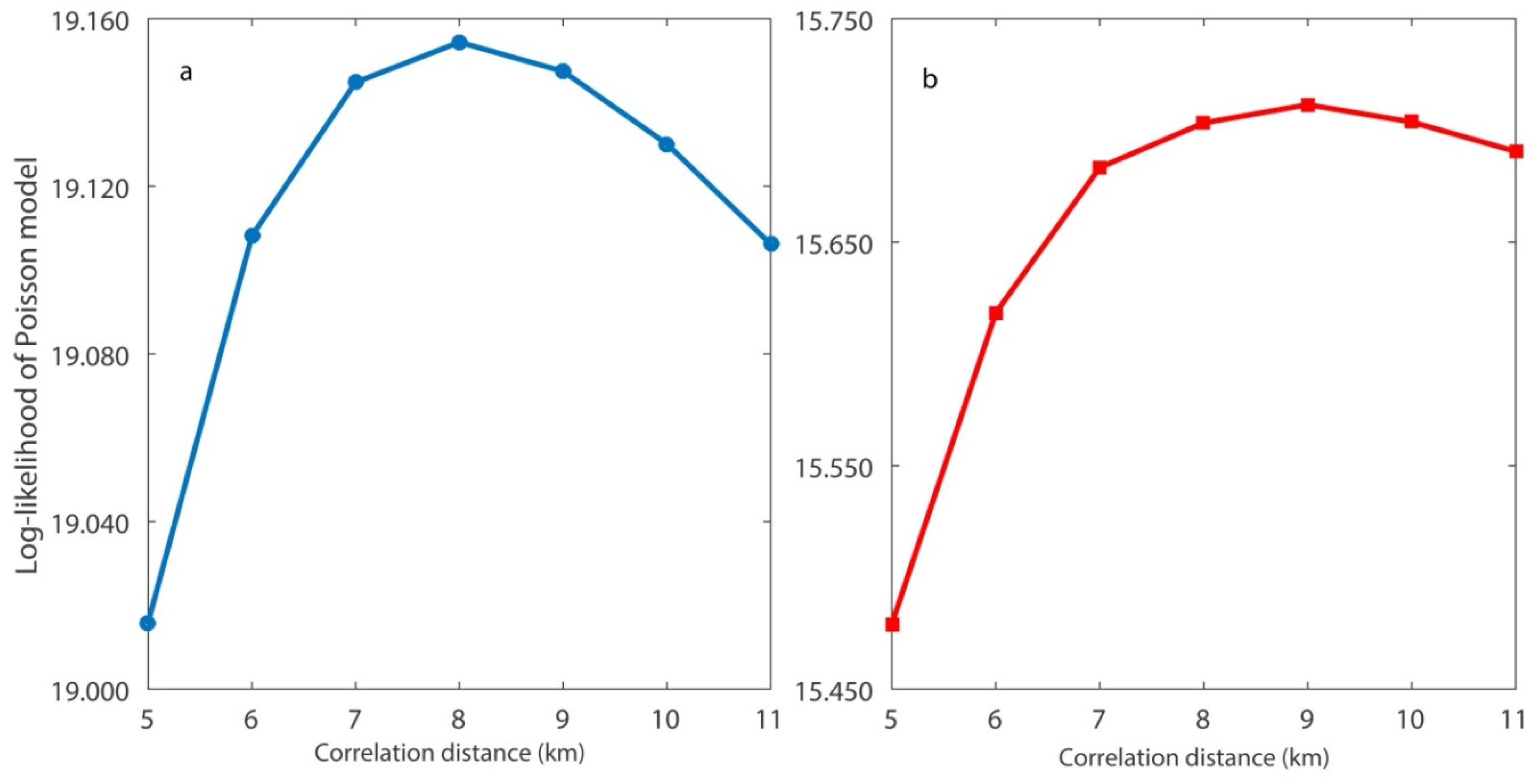
The spatial distribution of the background seismicity was estimated for the learning period with the smoothing method of Console et al. [25] following Frankel [24]. For the determination of the correlation distance c_d, the catalog with the 3919 events was divided in two subcatalogs containing an equal number of events, namely, 1960 and 1959 events, respectively. The division depends only on the number of events. The first subcatalog covers the period between the 1 January 2008 and the 6 November 2010 and the second subcatalog covers the rest of the learning period. A normal grid with nodes at distances of 2 km was used covering a rectangular area with side of 150 km far from the origin point (lat. 39.5$°$, lon. 25$°$) in each axis. The process carried out included the maximization of the likelihood of the seismicity contained in the second half of the catalog under the time-independent Poisson model estimated from the first half, and vice versa. The optimal values for the two periods were equal to 8 km and 9 km, respectively, as shown in Figure 2. The fact that these values are close indicates the stability in time of the spatial distribution of the seismic activity, despite the fact that there is some discrepancy between the duration of the two subcatalogs. 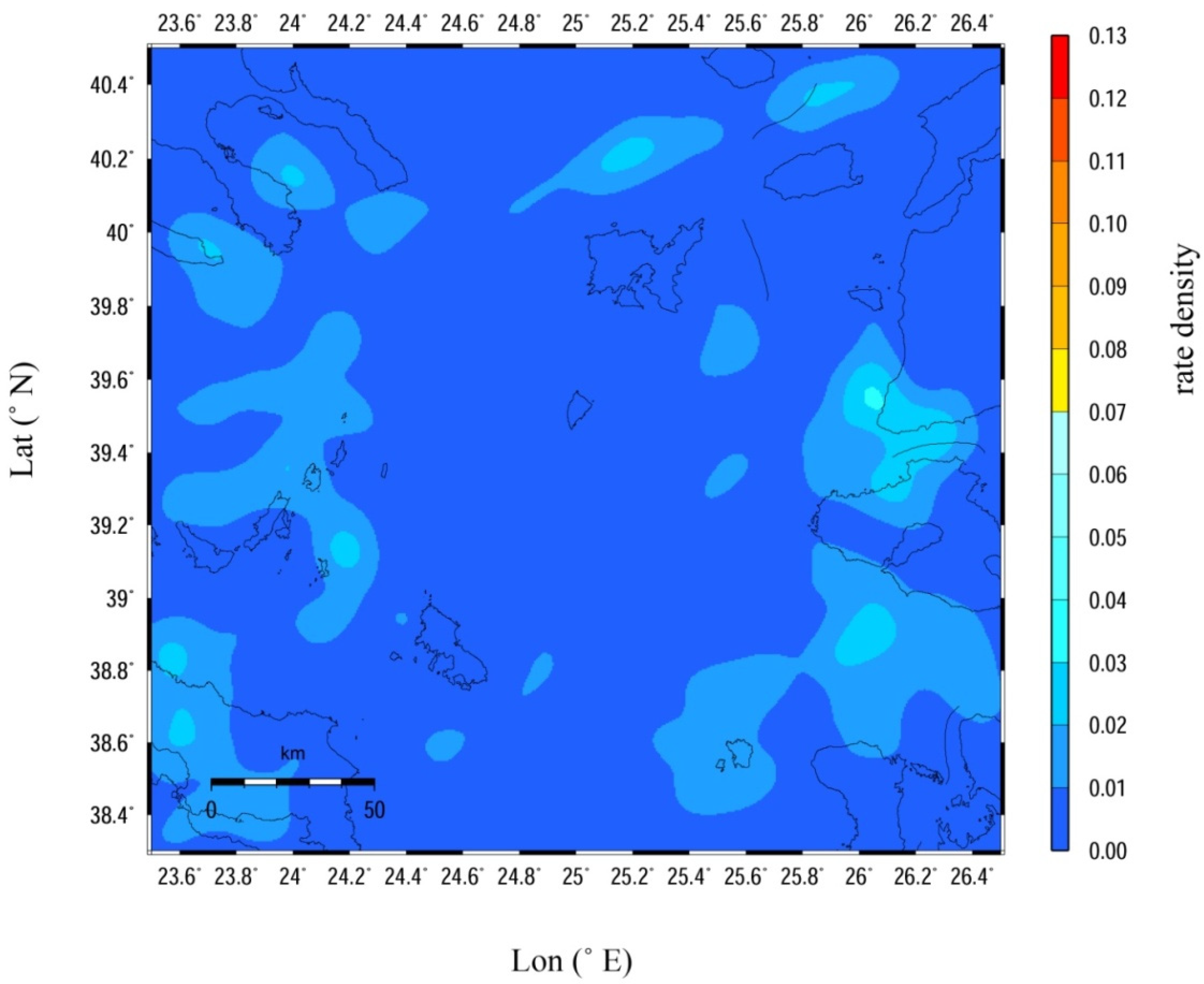The average of the two optimal values, i.e., c_d = 8.5 km, was chosen for the smoothed distribution shown in Figure 3.

In order to obtain a spatial distribution that does not comprise the triggered part of seismicity, we estimated the maximum-likelihood best-fit parameters of the ETAS model by progressively adjusting the background seismicity.

Table 2. Values obtained for the parameters of the epidemic model in the progressive adjustment of the background seismicity.

Parameters	Number of Iterations
	1st	2nd	3rd	4th	5th	6th	7th
k (daysp−1)	0.2275	0.2245	0.2245	0.2230	0.2230	0.2219	0.2218
d0 (km)	1.378	1.400	1.4115	1.4150	1.4250	1.4250	1.4256
q	1.9819	2.0178	2.0297	2.0347	2.0450	2.0450	2.0436
c (days)	0.0075	0.00725	0.00725	0.00725	0.00712	0.00712	0.00713
p	1.0306	1.0311	1.0309	1.0309	1.0309	1.0309	1.0309
α	0.3932	0.3931	0.3956	0.3956	0.3962	0.3962	0.3953
fr	0.321	0.324	0.322	0.321	0.322	0.325	0.325
lnL	46,849.32	46,995.06	46,995.45	46,995.73	46,996.02	46,996.11	46,996.17

shows the results yielded after seven consecutive iterations. The new smoothed seismicity distribution in the study area was obtained by means of the parameters that were derived after the final iteration (Figure 4).

Figure 3 and Figure 4 reveal the smoothed seismicity spatial distribution associated with the major regional faults. In the second map particularly, the seismicity is more scattered. Using the same color scale for a direct comparison between Figure 3 and Figure 4, we see that after the consecutive iterations there is not any single point associated with warm colors, meaning that the rate density is smoothed. The influence of the seismic excitation that occurred near the coast of northwestern Turkey during the first months of 2017 as well as the effect of the 2014 Samothraki sequence are partly eliminated. As expected, the spots along the North Aegean Trough are still present. The southeastern and southwestern boundaries of the study area also exhibit some degree of clustering since they are historically connected with increased seismic activity.

We then applied the epidemic model to retrospectively evaluate its performance. The original formulation of the ETAS model is intended for modeling aftershock sequences, but it may be extended to forecast the occurrence of stronger events. The testing period in our case is selected to start a few days before the occurrence of the 12 July 2017 M_w6.4 main shock, starting on the 1 June 2017, and lasting until the 31 July 2017. The choice of the testing period was adopted so that it began a few days before the main shock in order to test not only the performance of the aftershock activity but also the performance of the model towards the main shock. It was assumed that each forecast refers to seismicity starting at 0:00 and ending at 24:00 for every day of the testing period. The foreshock activity in the testing period of the first 11 days of June included only an event with M ≥ 2.7. This low foreshock activity influenced the forecasted occurrence probability for an event with M ≥ 6.0, which was found low at midnight, approximately 12 h before the occurrence of the main shock, and was equal to 0.4 × 10⁻⁶.

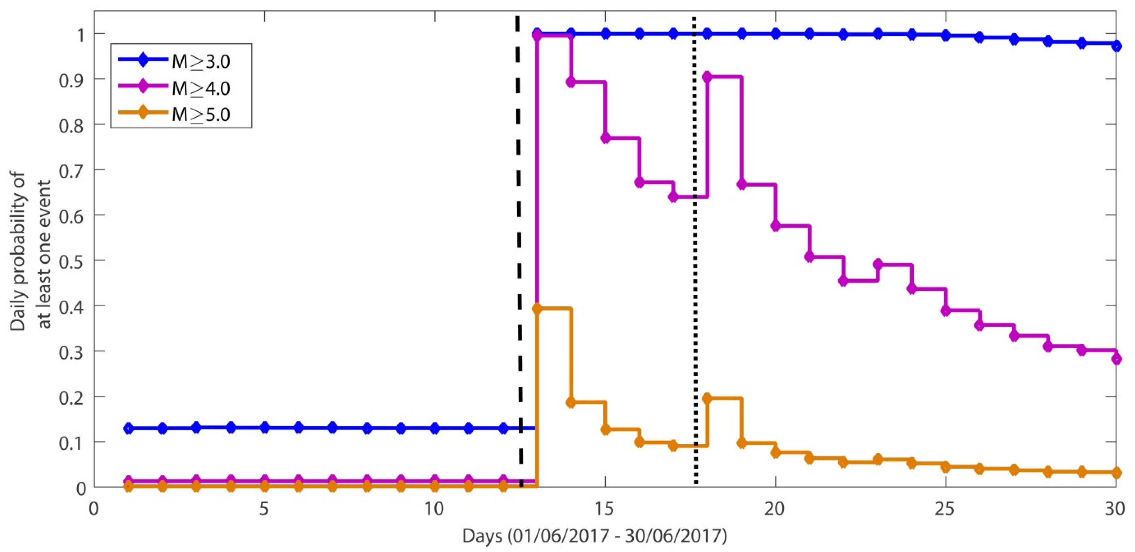
We calculated daily occurrence probabilities for several days before and after the main shock, 30 days in total, for three magnitude ranges (Figure 5). An abrupt increase in the daily probabilities appeared in relation to the first computations that were carried out approximately 12 h after the occurrence of the target event, and are marked by the dashed line. The occurrence probabilities became extremely high, particularly for M ≥ 3.0 earthquakes, which were assigned a daily occurrence probability equal to 1 for almost all of the remaining study period. On 13 June the occurrence of events with M ≥ 4.0 corresponded to a daily probability of occurrence equal to 0.995, whereas for those with M ≥ 5.0, the occurrence probability was equal to 0.393. The dotted line corresponds to the occurrence time of the M_w5.3 event on 17 June, the occurrence of which resulted in jumps in the plots of the occurrence probabilities for earthquakes with M ≥ 4.0 (prob = 0.904) and M ≥ 5.0 (prob = 0.195).

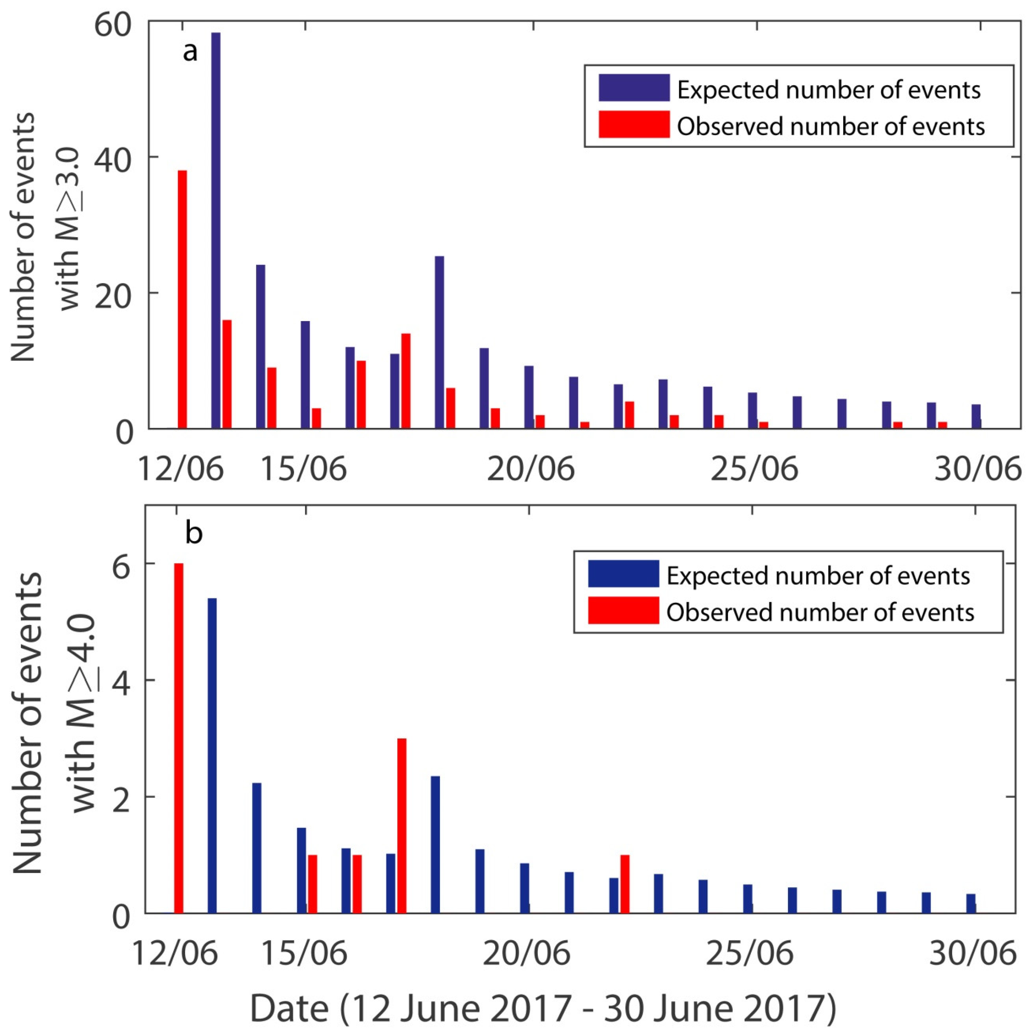
The observed and expected number of earthquakes with M ≥ 3.0 and M ≥ 4.0 are compared in Figure 6a,b, respectively. Given the absence of foreshocks at midnight, 12 h before the occurrence of the main shock, it is plausible that a small number of events is expected for both magnitude ranges. Then, on 13 June, particularly for earthquakes with M ≥ 3.0, the expected earthquake frequency increases rapidly. For most of the days, the expected number of events is larger than the observed one, but in general, the model manages to sufficiently predict the number of events. The sequence lacks earthquakes with M ≥ 4.0, as we see in Figure 6b. The predictions are not contradictory, though, since especially during the last ten days of June, the expected numbers range in low levels, under one expected event per day, between 0.33 and 0.85.

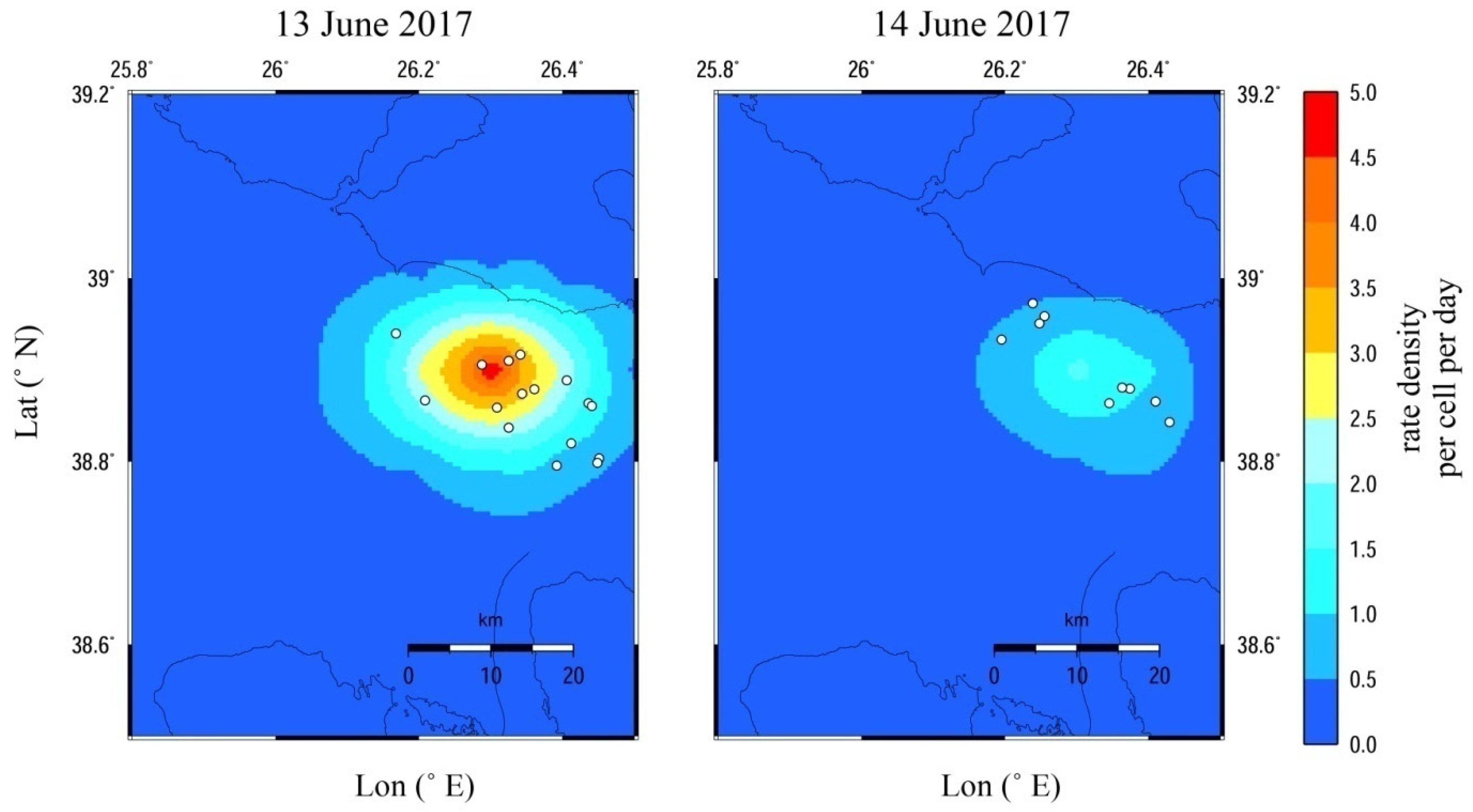
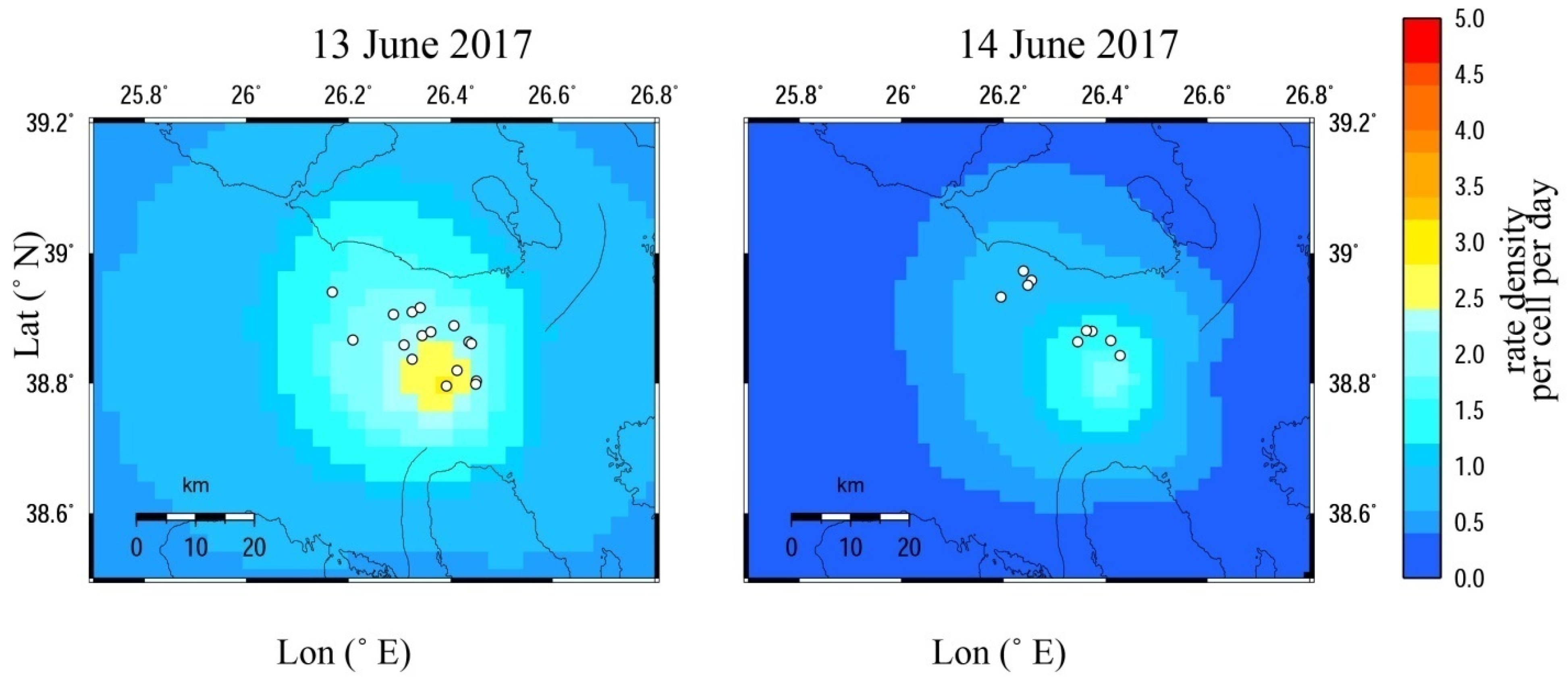
We then aimed to show the time-dependent seismicity related to the expected number of earthquakes with magnitudes of M ≥ 3.0 for a few days after the occurrence of the M_w6.4 Lesvos main shock on 12 June. For that reason, we divided the entire area into square cells of 0.1$°$ × 0.1$°$ in an attempt to examine if the spatial pattern of the expected earthquakes is in agreement with the earthquake’s epicentral distribution. As shown in the relevant maps (Figure 7), the spatial distribution of the expected number of events is in good agreement with the locations of the observed events on 13 and 14 June 2017. All of them are located in sites where the expected daily rate-density per cell is comparatively high. For a more detailed illustration, the maps are focused on an area south of Lesvos Island, where we anticipated intense aftershock activity.

In addition, with the qualitative assessment of the model performance, the quantitative evaluation included the generation of ROC diagrams by constructing a 2 × 2 contingency table. The initial date of the verification period coincided with the same date of the test phase, i.e., 1 June, and the final date was 31 July 2017. The study area was divided, as previously mentioned, into 713 square cells of 0.1$°$ × 0.1$°$ and 61 bins of 24 h each, resulting in 43,493 time–space cells. The magnitude threshold of the earthquakes for which forecasts are required was set equal to 3.0. One-hundred-twenty-seven (127) target events comprised the aforementioned period, the epicentral distribution of which is shown in Figure 8. The target events are concentrated in the offshore area south of Lesvos Island. For that reason, the map in Figure 9 focuses on a smaller part relative to the whole study area.

It may happen that two or more events, particularly those belonging in the magnitude range of [3.0, 3.2], occur in the same time–space cell of 0.1$°$ × 0.1$°$ lasting 24 h. It is more reasonable that when dealing with alarm-based forecasts, each cell of the time–space target volume is considered once, so that the total number of counts considered in the 2D binary matrix is identical to the total number of cells in the time–space volume. Thus, if two events occur in the same time–space bin, they must be counted as one observation and are considered as one success in the case that they are forecasted yes, and as one missed event in the case of being forecasted no. As a result, seventy-three (73) out of the one-hundred-twenty-seven (127) earthquakes with M ≥ 3.0 were the target events, while fifty-four (54) events were excluded from the computations.

When filling in the contingency tables, a forecast was defined in a certain cell if the occurrence rate of earthquakes with magnitude greater than 3.0 exceeded the threshold value r. The calculations were performed every 24 h in cells of 0.1$°$ × 0.1$°$. The results for various occurrence-rate thresholds between 0.0005 and 0.03 are presented in

Table 3. Contingency tables for the clustering model related to the testing period between 1 June 2017–31 July 2017 using various occurrence-rate thresholds for events with M ≥ 3.0. Events that occur in the same time–space bin are counted as one observation.

Forecasted	Observed
r = 0.03	Yes	No
Yes	$a=57$	$b=1602$
No	$d=16$	$c=\mathrm{41,818}$
r = 0.02
Yes	$a=57$	$b=2323$
No	$d=16$	$c=\mathrm{41,097}$
r = 0.01
Yes	$a=57$	b = 4226
No	$d=16$	$c=\mathrm{39,194}$
r = 0.005
Yes	$a=57$	$b=7542$
No	$d=16$	$c=\mathrm{35,878}$
r = 0.001
Yes	$a=60$	$b=\mathrm{20,735}$
No	$d=13$	$c=\mathrm{22,685}$
r = 0.0005
Yes	$a=67$	$b=\mathrm{30,488}$
No	$d=6$	$c=\mathrm{12,932}$

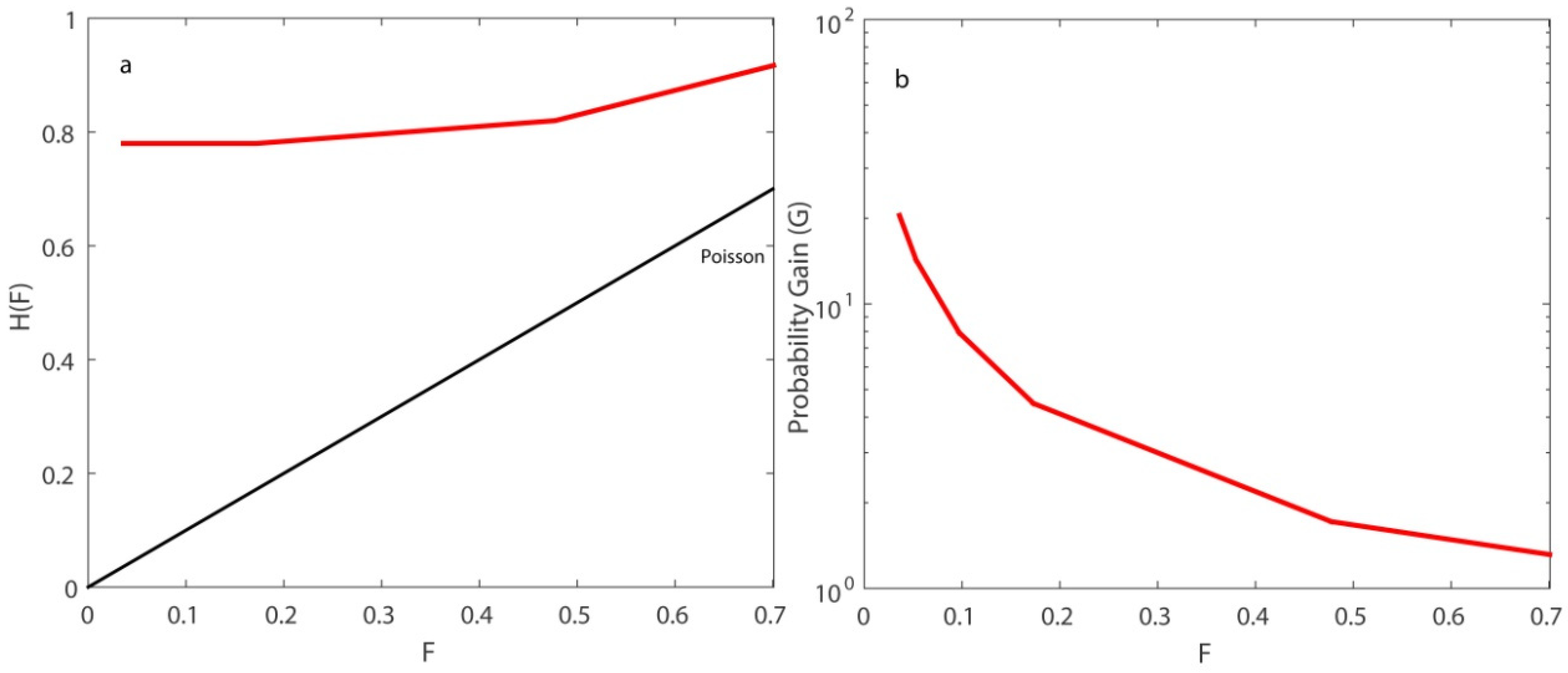
. In most cases, except for r = 0.03, the vast majority of cells are empty. Based on the contingency tables, the values of the hit rate H and the false-alarm rate F were computed in order to be employed for the creation of the ROC diagrams. For each occurrence-rate threshold, a different point (H, F) was plotted in the ROC diagram (Figure 9a). In general, when increasing the rate threshold r, the H and F decrease, i.e., both the fraction of events that occurred in an alarm cell and the fraction of false alarms decrease. This happens because the predictions are stricter. It is not that common for a cell to be assigned a high occurrence probability, meaning that alarms are more infrequent. For example, when r = 0.03, only 1659 out of the 43,493 cells, i.e., 3.8 per cent of the cells contain alarms. Consequently, that leads to lower false alarms but also to a lower percentage of hit rates.

In the examined case, we can make a remarkable observation concerning the stability of the hit-rate values. Specifically, for occurrence-rate thresholds between 0.005 and 0.03, H was stable and equal to 0.78. That means 57 out of 73 earthquake targets were predicted since they belonged to cells with high occurrence rates, greater than 0.03, while the remaining 16 of them belonged to cells with very low occurrence rates, lower than 0.005. The remaining earthquakes would be very difficult to predict, only by significantly reducing the occurrence-rate threshold. A total 67 out of the 73 target events were predicted when decreasing the rate threshold to r = 0.0005. However, this would significantly increase the false-alarm rate at 70 per cent.

The difference between H and F could be considered as a measure of the randomness of the predictions. The biggest difference between them was observed for r = 0.03, H − F = 0.744 (

Table 4. Statistical tools applied for various occurrence-rate thresholds.

r = 0.03	r = 0.02	r = 0.01	r = 0.005	r = 0.001	r = 0.0005
H = 0.78	H = 0.78	H = 0.78	H = 0.78	H = 0.82	H = 0.92
F = 0.036	F = 0.053	F = 0.097	F = 0.173	F = 0.477	F = 0.701
R = 0.033	R = 0.034	R = 0.0129	R = 0.007	R = 0.023	R = 0.002
R’ = 0.744	R’ = 0.727	R’ = 0.684	R’ = 0.607	R’ = 0.344	R’ = 0.217
G = 20.47	G = 14.27	G = 7.93	G = 4.47	G = 1.72	G = 1.32

). In all the examined cases, even when the false-alarm rate was at its highest value, for r = 0.0005, the predictions were far from random. This can be easily shown in Figure 10a.

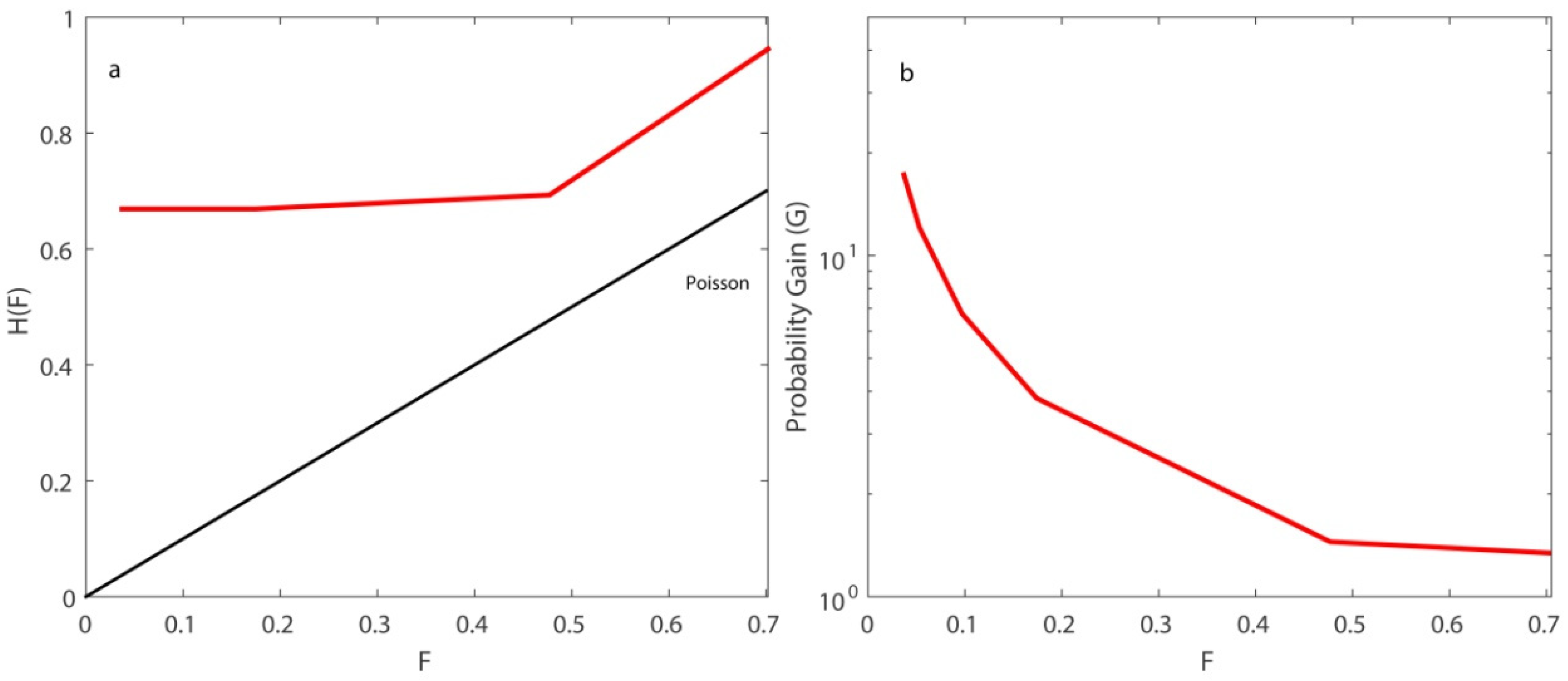
The assessment of the ETAS model was also carried out through the probability gain G. Figure 9b shows the results of G versus F. When the false-alarm rate increases, G decreases. The values of G range from a few tens to some units. Regarding the two alternative expressions of the R-score, R’ obtained higher values than R [15]. This mainly happened due to their formulations, because d was much smaller than b, and b was smaller than c. For r = 0.03, the value of G was quite high, equal to 20.47. At the same time, the value of R’ was maximized. For that occurrence-rate threshold, the real rate of successes was equal to 0.034. This value resulted from the fact that 57 events were successfully estimated over 1659 alarms. In that way, not only were the space–time cells that were rightly expected to accommodate an earthquake taken into account, but also those that, according to the model, corresponded to an earthquake, but in reality an event did not ultimately occur.

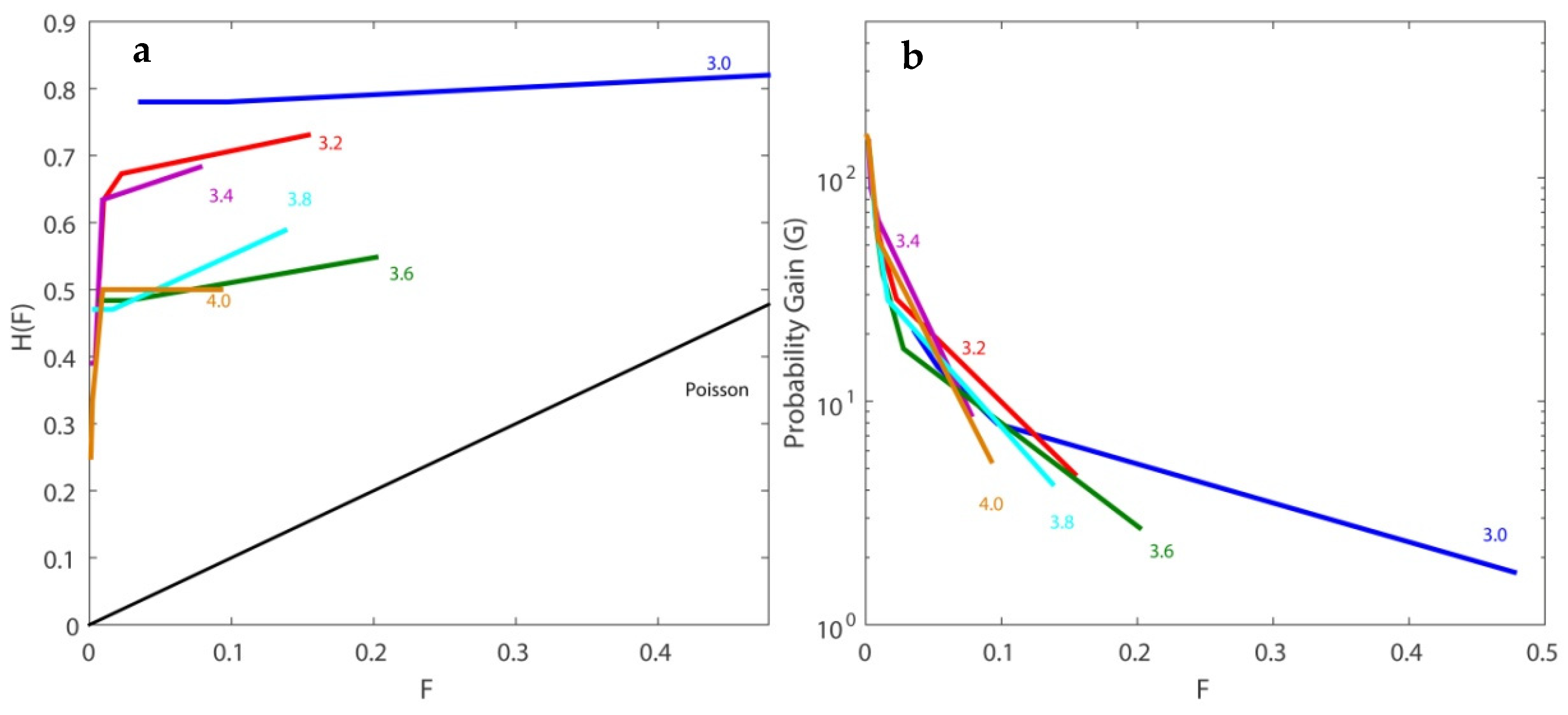
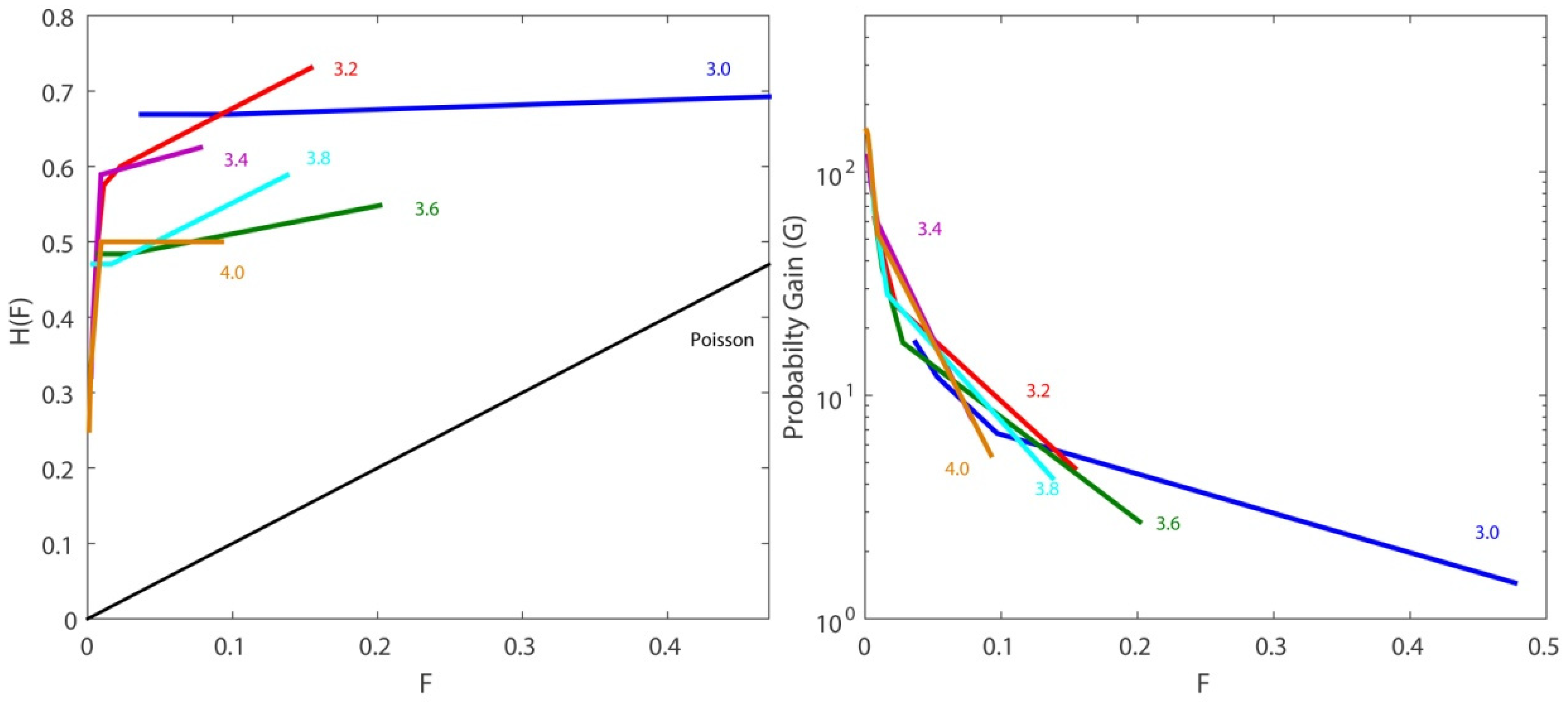
For further investigating the model’s performance, different magnitude thresholds over the completeness magnitude were tested, from 3.0 up to 4.0 in steps of 0.2 magnitude units. This resulted in modifications to the contingency table. As a result, the corresponding ROC diagrams and the probability-gain diagrams also changed (Figure 10). The higher the threshold magnitude, the smaller the number of successes and false alarms. In any case, all predictions were far from being random. For example, for r = 0.001 and a magnitude threshold equal to 4.0, the real success rate was 0.0014 (6 successes out of 4027 alarms) towards a random occurrence rate equal to 0.0002 (12 events over 43,493 space–time cells). For a magnitude threshold equal to 3.0 and r = 0.01, the real success rate was 0.013 towards a random occurrence rate equal to 0.0016.

Regarding the branching ratio, the computed value of ρ for the suggested model was equal to 0.267, indicating the stability of the model.

For comparison and a more profound investigation, the alternative approach was also followed, where every event was considered in the computations irrespective of whether an event had previously occurred in the same time–space cell. That means the target events with M ≥ 3.0 were 127. For comparison we refer to the Appendix A.

6. Discussion and Conclusions

The performance of an epidemic model of clustered seismicity in the northern Aegean Sea area was retrospectively evaluated. The absence of foreshocks is responsible for the low probability of occurrence for an event with M ≥ 6.0 a few hours before the occurrence of the Mw6.4 Lesvos main shock. The performance of the model regarding the aftershock sequence was quite satisfactory, although the observed aftershocks were fewer than those anticipated by the model. The spatial distribution of the expected seismicity rate agreed well with the spatial distribution of the observed seismicity during 13 and 14 June 2017, since all of them were located in sites where the expected daily rate-density per cell was high.

The quantitative assessment of the model deemed 127 target events with M ≥ 3.0 whose occurrence in June and July 2017 were investigated in terms of probabilities through the construction of contingency tables, the application of statistical criteria and the generation of ROC diagrams. We pursued two different approaches, in which events that occurred in the same time–space bin were either counted as one observation or as different ones. Thus, in the first case, there were 73 target events compared to 127 in the second case.

We examined earthquake occurrence in both approaches through various occurrence-probability thresholds r. High threshold rates resulted in high values of probability gain and low values of false-alarm rate. Although we expected that the values of H would also decrease as r increased, there was a remarkable stability for several occurrence-probability thresholds. The optimal solution should ensure that not only the rate of successes is high but also the rate of false alarms is low. For example, for r = 0.03, only a small percentage of 3.6 per cent corresponded to earthquakes that the model predicted but that did not occur. We considered this value of the occurrence-rate threshold as the most suitable towards that direction, predicting 78 per cent in the first case and 67 per cent of the target events in the second case, while simultaneously maintaining false alarms at very low levels.

We then compared the model’s performance with a clustering model previously applied in the Greek territory, details of which are provided in

Table 5. Estimated parameters of the clustering model applied in the Greek territory.

Time Span	1 January 2010–31 May 2017
Testing period	1 June 2017–31 July 2017
Study region	lat. 34.0°–42° N, lon. 19.0°–29.5° E
Magnitude threshold	2.7
Correlation distance(km)	14.5
k (daysp−1)	0.2218
d0 (km)	1.4256
q	2.0436
c (days)	0.0071
p	1.0309
a	0.3953
fr	0.3250

. As expected, the value of the correlation distance in the northern Aegean area was smaller since it referred to a much smaller area. This may also be attributed to the slightly smaller magnitude threshold adopted in this study. We observed, though, that the values of the estimated parameters in both cases were quite close, indicating similar spatio-temporal behavior. The calculated value of the branching ratio was equal to ρ = 0.267, showing that the branching process was stable. The two compared values were similar since they were derived from almost equal parameter estimations.

The daily probabilities of occurrence of having at least one event with M ≥ 6.0 in the study area at midnight on 12 June was equal to 1.1 × 10⁻³. The respective probability for the main shock, when applying the epidemic clustering model in the Greek territory, was almost 3000 times greater than the estimate for the northern Aegean area. A possible interpretation is probably either the presence or absence of foreshocks. In the testing period, during the first eleven days of June, 51 events with Μ ≥ M_th occurred before the main shock, while in the northern Aegean area only one event is included in the catalog. This also might be attributed to the calculation area of the daily probability for an event with Μ ≥ 6.0, which included the whole study area and not only the particular cell corresponding to the main shock. Larger study areas are probably associated with larger occurrence probabilities.

The maps depicting the time-dependent seismicity were created based on a grid of square cells with dimensions 0.2$°$ × 0.2$°$ (Figure 11) while the corresponding northern Aegean area was divided into square cells of 0.1$°$ × 0.1$°$ because of its smaller dimensions. The spatial patterns based on the two different models were similar, as anticipated based on the similar values of the estimated parameters. Yet, the clustering model exclusively developed for the northern Aegean area provided a more concentrated and focused pattern around higher densities (marked with orange and red colors in Figure 7).

Concluding, the performance of the northern Aegean clustering model was retrospectively verified by comparing the expected and observed earthquake numbers and through various statistical criteria. Target events with Μ ≥ 3.0 were predicted with high probabilities and at the same time, the model did not produce a great deal of false alarms. The encouraging retrospective results that emerged from our analysis and the forecast-verification procedures indicate that the clustering model is able to provide reliable information regarding short-term probabilities of occurrence of future events. As a next step, it could be thus used as a contribution to real-time forecasts, even for practical purposes.

References

1. Utsu, T.; Ogata, Y.; Matsu’ura, R.S. The centenary of the Omori formula for a decay law of aftershock activity. J. Phys. Earth 1995, 43, 1–33. [Google Scholar] [CrossRef]
2. Kagan, Y.Y.; Jackson, D.D. Spatial aftershock distribution: Effect of normal stress. J. Geophys. Res. 1998, 103, 24453–24467. [Google Scholar] [CrossRef] [Green Version]
3. Meltzner, A.J.; Wald, D.J. Foreshocks and aftershocks of the great 1857 California earthquake. Bull. Seismol. Soc. Am. 1999, 89, 1109–1120. [Google Scholar] [CrossRef]
4. Dreger, D.; Savage, B. Aftershocks of the 1952 Kern County, California, earthquake sequence. Bull. Seismol. Soc. Am. 1999, 89, 1094–1108. [Google Scholar] [CrossRef]
5. Ogata, Y. Statistical models for earthquake occurrences and residual analysis for point processes. J. Am. Stat. Assoc. 1988, 83, 9–27. [Google Scholar] [CrossRef]
6. Ogata, Y. Space–time point-process models for earthquake occurrences. Ann. Inst. Stat. Maths 1998, 50, 379–402. [Google Scholar] [CrossRef]
7. Console, R.; Murru, M. A simple and testable model for earthquake clustering. J. Geophys. Res. 2001, 106, 8699–8711. [Google Scholar] [CrossRef]
8. Console, R.; Murru, M.; Lombardi, A.M. Refining earthquake clustering models. J. Geophys. Res. 2003, 108, 2468. [Google Scholar] [CrossRef]
9. Helmstetter, A.; Jackson, D.D.; Kagan, Y.Y. Comparison of short-term and time-independent earthquake forecast models for southern California. Bull. Seismol. Soc. Am. 2006, 96, 90–106. [Google Scholar] [CrossRef] [Green Version]
10. Zhuang, J.; Werner, W.J.; Hainzl, S.; Harte, D.; Zhou, S. Basic models of seismicity: Spatiotemporal modes. Commun. Online Resour. Stat. Seismol. Anal. 2011, 20. [Google Scholar] [CrossRef]
11. Marzocchi, W.; Lombardi, A.M. Real-time forecasting following a damaging earthquake. Geophys. Res. Lett. 2009, 36, L21302. [Google Scholar] [CrossRef]
12. Lombardi, A.M.; Cocco, M.; Marzocchi, W. On the increase of background seismicity rate during the 1997–1998 Umbria-Marche, central Italy, sequence: Apparent variation or fluid-driven triggering? Bull. Seismol. Soc. Am. 2010, 100, 1138–1152. [Google Scholar] [CrossRef] [Green Version]
13. Zhuang, J. Next–day earthquake forecasts by using the ETAS model. Earth Planets Space 2011, 63, 207–216. [Google Scholar] [CrossRef] [Green Version]
14. Murru, M.; Zhuang, J.; Console, R.; Falcone, G. Short-term earthquake forecasting experiment before and during the L’Aquila (central Italy) seismic sequence of April 2009. Ann. Geophys. 2014, 57, S0649. [Google Scholar] [CrossRef]
15. Murru, M.; Console, R.; Falcone, G. Real time earthquake forecasting in Italy. Tectonophysics 2009, 470, 214–223. [Google Scholar] [CrossRef]
16. Console, R.; Murru, M.; Falcone, G. Probability gains of an epidemic-type aftershock sequence model in retrospective forecasting of m ≥ 5 earthquake in Italy. J. Seismol. 2010, 14, 9–26. [Google Scholar] [CrossRef] [Green Version]
17. Nanjo, K.Z.; Tsuruoka, H.; Yokoi, S.; Ogata, Y.; Falcone, G.; Hirata, N.; Ishigaki, Y.; Jordan, T.H.; Kasahara, K.; Obara, K.; et al. Predictability study on the aftershock sequence following the 2011 Tohoku-Oki, Japan, earthquake: First results. Geophys. J. Int. 2012, 191, 653–658. [Google Scholar] [CrossRef] [Green Version]
18. Ogata, Y.; Katsura, K.; Falcone, G.; Nanjo, K.Z.; Zhuang, J. Comprehensive and topical evaluations of earthquake forecasts in terms of number, time, space, and magnitude. Bull. Seismol. Soc. Am. 2013, 103, 1692–1708. [Google Scholar] [CrossRef]
19. Jordan, T. Earthquake predictability, brick by brick. Seismol. Res. Lett. 2006, 77, 3–6. [Google Scholar] [CrossRef]
20. Marzocchi, W.; Taroni, M.; Falcone, G. Earthquake forecasting during the complex Amatrice-Norcia seismic sequence. Sci. Adv. 2017, 3, e1701239. [Google Scholar] [CrossRef] [Green Version]
21. Schorlemmer, D.; Werner, M.J.; Marzocchi, W.; Jordan, T.H.; Yosihiko, O.; Jackson, D.D.; Mak, S.; Rhoades, D.A.; Gerstenberger, M.C.; Hirata, N.; et al. The collaboratory for the study of earthquake predictability: Achievements and priorities. Seismol. Res. Lett. 2018, 89, 1305–1313. [Google Scholar] [CrossRef] [Green Version]
22. Taroni, M.; Marzocchi, W.; Schorlemmer, D.; Werner, M.; Zechar, J.D.; Wiemer, S.; Heiniger, L.; Euchner, F. Prospective CSEP evaluation of 1-day, 3-month, and 5-year earthquake forecasts for Italy. Seismol. Res. Lett. 2018, 89, 1251–1261. [Google Scholar] [CrossRef] [Green Version]
23. Mangira, O.; Console, R.; Papadimitriou, E.; Murru, M.; Karakostas, V. The short-term seismicity of the Central Ionian Islands (Greece) studied by means of a clustering model. Geophys. J. Int. 2020, 220, 856–875. [Google Scholar] [CrossRef]
24. Frankel, A. Mapping seismic hazard in the central and eastern United States. Seismol. Res. Lett. 1995, 66, 8–21. [Google Scholar] [CrossRef]
25. Console, R.; Jackson, D.D.; Kagan, Y.Y. Using the ETAS model for catalog declustering and seismic background assessment. Pure Appl. Geophys. 2010, 167, 819–830. [Google Scholar] [CrossRef] [Green Version]
26. Zhuang, J.; Ogata, Y.; Vere-Jones, D. Stochastic declustering of space-time earthquake occurrence. J. Am. Stat. Assoc. 2002, 97, 369–380. [Google Scholar] [CrossRef]
27. Marsan, D.; Longliné, O. Extending earthquakes’ reach through cascading. Science 2008, 319, 1076–1079. [Google Scholar] [CrossRef] [Green Version]
28. Ogata, Y. Estimation of the parameters in the modified Omori formula for aftershock sequences by the maximum likelihood procedure. J. Phys. Earth 1983, 31, 115–124. [Google Scholar] [CrossRef]
29. Kagan, Y.Y.; Jackson, D.D. Long-term earthquake clustering. Geophys. J. Int. 1991, 104, 117–133. [Google Scholar] [CrossRef] [Green Version]
30. Zhuang, J.; Ogata, Y.; Vere-Jones, D. Analyzing earthquake clustering features by using stochastic reconstruction. J. Geophys. Res. 2004, 109, B05301. [Google Scholar] [CrossRef] [Green Version]
31. Zhuang, J.; Chang, C.-P.; Ogata, Y.; Chen, Y.-I. A study of the background and clustering seismicity in the Taiwan region by using a point process model. J. Geophys. Res. 2005, 110, B05S18. [Google Scholar] [CrossRef] [Green Version]
32. Ogata, Y.; Zhuang, J. Space–time ETAS models and an improved extension. Tectonophysics 2006, 413, 13–23. [Google Scholar] [CrossRef]
33. Hainzl, S.; Christophersen, A.; Enescu, B. Impact of earthquake rupture extensions on parameter estimations of point process models. Bull. Seismol. Soc. Am. 2008, 98, 2066–2072. [Google Scholar] [CrossRef]
34. Werner, M.J.; Helmstetter, A.; Jackson, D.D.; Kagan, Y.Y. High-resolution long-term and short-term earthquake forecasts for California. Bull. Seismol. Soc. Am. 2011, 101, 1630–1648. [Google Scholar] [CrossRef] [Green Version]
35. Aki, K. Maximum likelihood estimate of b in the formula log n = a−bm and its confidence limits. Bull. Earthq. Res. Inst. 1965, 43, 99–103. [Google Scholar]
36. Console, R. Testing earthquake forecast hypotheses. Tectonophysics 2001, 338, 261–268. [Google Scholar] [CrossRef]
37. Kossobokov, V.G. Testing earthquake prediction methods: The West Pacific short-term forecast of earthquakes with magnitude MwHRV ≥ 5.8. Tectonophysics 2006, 413, 25–31. [Google Scholar] [CrossRef]
38. Chen, C.-C.; Rundle, J.B.; Li, H.-C.; Holliday, J.R.; Nanjo, K.Z.; Turcotte, D.L.; Tiampo, K.F. From tornados to earthquakes: Forecast verification for binary events applied to the 1999 Chi-Chi, Taiwan, Earthquake. Terr. Atmos. Ocean. Sci. 2006, 17, 503–516. [Google Scholar] [CrossRef] [Green Version]
39. Zechar, J.D.; Jordan, T.H. Testing alarm–based earthquake predictions. Geophys. J. Int. 2007, 172, 715–724. [Google Scholar] [CrossRef] [Green Version]
40. Holliday, J.R.; Nanjo, K.Z.; Tiampo, K.F.; Rundle, J.B.; Turcotte, D.L. Earthquake forecasting and its verification, nonlinear processes in geophysics. Eur. Geosci. Union 2005, 12, 965–977. [Google Scholar]
41. Hanssen, A.W.; Kuipers, A.J.W. On the relationship between frequency of rain and various meteorological parameters. Meded. Verh. 1965, 81, 2–15. [Google Scholar]
42. Harte, D.; Vere-Jones, D. The entropy score and its uses in earthquake forecasting. Pure Appl. Geophys. 2005, 162, 1229–1253. [Google Scholar] [CrossRef]
43. Shi, Y.; Liu, J.; Zhang, G. An evaluation of Chinese annual earthquake predictions, 1990–1998. J. Appl. Probab. 2001, 38, 222–231. [Google Scholar] [CrossRef] [Green Version]
44. Aki, K. A Probabilistic Synthesis of Precursory Phenomena. In Earthquake Prediction; Simpson, D.W., Richards, P.G., Eds.; American Geophysical Union: Washington, DC, USA, 1981; pp. 556–574. [Google Scholar]
45. Sornette, D.; Helmstetter, A. Occurrence of finite-time singularities in epidemic models of rupture, earthquakes and starquakes. Phys. Rev. Lett. 2002, 89, 158501. [Google Scholar] [CrossRef] [Green Version]
46. Sornette, D.; Werner, M.J. Constraints on the size of the smallest triggering earthquake from the epidemic–type aftershock sequence model, Bath’s law, and observed aftershock sequences. J. Geophys. Res. 2005, 110, D15. [Google Scholar] [CrossRef] [Green Version]
47. Console, R.; Falcone, G.; Karakostas, V.; Murru, M.; Papadimitriou, E.; Rhoades, D. Renewal models and coseismic stress transfer in the Corinth Gulf Greece, fault system. J. Geophys. Res. 2013, 118, 3655–3673. [Google Scholar] [CrossRef]
48. Zhuang, J.; Harte, D.; Werner, M.J.; Hainzl, S.; Zhou, S. Basic models of seismicity: Temporal models. Commun. Online Resour. Stat. Seismol. Anal. 2012, 42. [Google Scholar] [CrossRef]
49. Papazachos, B.C.; Papadimitriou, E.E.; Kiratzi, A.A.; Papazachos, C.B.; Louvari, E.K. Fault plane solutions in the Aegean Sea and the surrounding area and their tectonic implications. Boll. Geofis. Teor. Appl. 1998, 39, 199–218. [Google Scholar]
50. Le Pichon, X. Land-Locked Oceanic Basins and Continental Col-Lision: Eastern Mediterranean as a Case Example. In Mountain Building Processes; Hsü, K., Ed.; Academic Press: New York, NY, USA, 1982; p. 201. [Google Scholar]
51. Papazachos, B.C.; Comninakis, P.E. Geophysical and tectonic features of the Aegean arc. J. Geophys. Res. 1971, 76, 8517–8533. [Google Scholar] [CrossRef]
52. Evangelidis, C.P. Imaging supershear rupture for the 2014 Mw6.9 Northern Aegean earthquake by back projection of strong motion waveforms. Geophys. Res. Lett. 2015, 42, 307–315. [Google Scholar] [CrossRef]
53. Kiratzi, A.; Tsakiroudi, E.; Benetatos, C.; Karakaisis, G. The 24 May 2014 (Mw6.8) earthquake (North Aegean Trough): Spatiotemporal evolution, source and slip model from teleseismic data. Phys. Chem. Earth 2016, 95, 85–100. [Google Scholar] [CrossRef]
54. Papadimitriou, P.; Kassaras, I.; Kaviris, G.; Tselentis, A.; Voulgaris, N.; Lekkas, E.; Chouliaras, G.; Evangelidis, C.; Pavlou, K.; Kapetanidis, V.; et al. The 12th June 2017 Mw = 6.3 Lesvos earthquake from detailed seismological observations. J. Geodyn. 2018, 115, 23–42. [Google Scholar] [CrossRef]
55. Aristotle University of Thessaloniki Seismological Network Permanent Regional Seismological Network Operated by the Aristotle University of Thessaloniki. International Federation of Digital Seismograph Networks, Other/Seismic Network. 1981. Available online: https://doi.org/10.7914/SN/HT (accessed on 1 January 2021).
56. Mesimeri, M.; Kourouklas, C.; Papadimitriou, E.; Karakostas, V.; Kementzetzidou, D. Analysis of microseismicity associated with the 2017 seismic swarm near the Aegean coast of NW Turkey. Acta Geophys. 2018, 66, 479–495. [Google Scholar] [CrossRef]
57. Wiemer, S.; Wyss, M. Minimum magnitude of completeness in earthquake catalogs: Examples from Alaska, the western US and Japan. Bull. Seismol. Soc. Am. 2000, 90, 859–869. [Google Scholar] [CrossRef]
58. Shi, Y.; Bolt, A. The standard error of the magnitude-frequency b-value. Bull. Seismol. Soc. Am. 1982, 72, 1677–1687. [Google Scholar] [CrossRef]
59. Wessel, P.; Smith, W.H.F.; Scharroo, R.; Luis, J.; Wobbe, F. Generic mapping tools: Improved version released. EOS Trans. Am. Geophys. Union 2013, 94, 409–410. [Google Scholar] [CrossRef] [Green Version]
Figure 1. Epicentral distribution of earthquakes with Μ ≥ 2.6 that occurred from January 2008 to December 2018. Events with 2.6 ≤ Μ < 4.0, 4.0 ≤ Μ < 5.0 and 5.0 ≤ Μ < 6.0 are depicted with white, orange and magenta, circles, respectively. The events of 2014 (Mw6.9) and that of 2017 (Mw6.4) are depicted with yellow stars.
Axioms 11 00249 g001
Figure 2. (a) Plot of the likelihood of the second part of the catalog under the time-independent Poisson model created from the first part of the catalog, versus different values of the cd parameter of the smoothing algorithm. (b) Equivalent plot for the likelihood of the first part of the catalog with respect to the second.
Axioms 11 00249 g002
Figure 3. Smoothed seismicity distribution in the study area (1 January 2008–31 May 2017) obtained by the smoothing algorithm applied to the raw catalog with a correlation distance of cd = 8.5 km. The color scale represents the number of events occurred in cells of 2 km × 2 km wide over the total duration of the catalog.
Axioms 11 00249 g003
Figure 4. Smoothed seismicity distribution of the study area (1 January 2008–31 May 2017) obtained by the smoothing algorithm applied to the weighted catalog with a correlation distance of cd = 8.5 km. The color scale represents the number of events occurred in cells of 2 km × 2 km over the total duration of the catalog.
Axioms 11 00249 g004
Figure 5. Daily occurrence probabilities of at least one event with M ≥ 3.0, M ≥ 4.0 and M ≥ 5.0 with blue, violet, and orange lines, respectively, for the period 1 June 2017–30 June 2017. The dashed line corresponds to the occurrence time of the Mw6.4, 12 June 2017 main shock. The dotted line corresponds to the occurrence time of the Mw5.3 aftershock on the 17 June.
Axioms 11 00249 g005
Figure 6. (a) Expected (blue bars) and observed (red bars) number of events with M ≥ 3.0 per day, under the ETAS model with the best-fit parameters. (b) The same as in (a) but with M ≥ 4.0.
Axioms 11 00249 g006
Figure 7. Expected daily number of events per cell of 0.1° × 0.1° of events with M ≥ 3.0 on 13 and 14 June. The computations are performed at midnight of each day. The white circles show the epicenters of the aftershocks observed on that certain day.
Axioms 11 00249 g007
Figure 8. Epicentral distribution of the 127 target events with M ≥ 3.0 that occurred during the testing period (June–July 2017). Events with 3.0 M < 4.0 ,   4.0 M < 5.0 ,   5.0 M < 6.0 are depicted with white, orange and magenta circles, respectively. The Mw6.4 event of 12 June 2017 is depicted with a yellow star.
Axioms 11 00249 g008
Figure 9. (a) Values of the hit rate H versus the false-alarm rate F. Each value of F corresponds to a different threshold rate for issuing alarms. Events that occur in the same time–space bin are counted as one observation. Random forecasts correspond to the black line. (b) Same as in (a), for the probability gain G, computed on the whole space–time volume.
Axioms 11 00249 g009
Figure 10. (a) Values of the hit rate H versus the false-alarm rate F for different magnitude thresholds. Each value of F corresponds to a different threshold rate for issuing alarms. Events that occur in the same time–space bin are counted as one observation. Random forecasts correspond to the black line. (b) Same as in (a) for the probability gain G, computed on the whole space–time volume.
Axioms 11 00249 g010
Figure 11. Expected daily number of earthquakes with M ≥ 3.0 per cell of 0.2° × 0.2° on 13 and 14 June based on the Greek territory clustering model. The computations are performed at midnight of each day. The white circles show the epicenters of the aftershocks occurred on the certain day.
Axioms 11 00249 g011