
Development of a Model for Evaluating the Efficiency of Transport Companies: PCA–DEA–MCDM Model

 ,
, 

Abstract
1. Introduction
2. Literature Review
2.1. Review of Applying the DEA Method for Evaluating the Efficiency in the Field of Transport
2.2. Review of Applying the PCA–DEA Model for Evaluating the Efficiency in the Field of Transport and the Supply
2.3. Review of Applying Integrated Models in the Field of Transport
2.4. A Review of Studies of Pandemic Impact on Transport and the Supply Chain
3. Methodology
3.1. DEA Model
3.2. PCA Model
- Standardization of variables;
- Computation of the matrix of correlations between all initial standardized variables;
- Finding the eigenvalues of the principal components;
- Rejection of the components that are carriers of a proportionally small share of variance (usually the first several components carry 80–90% of the total variance).
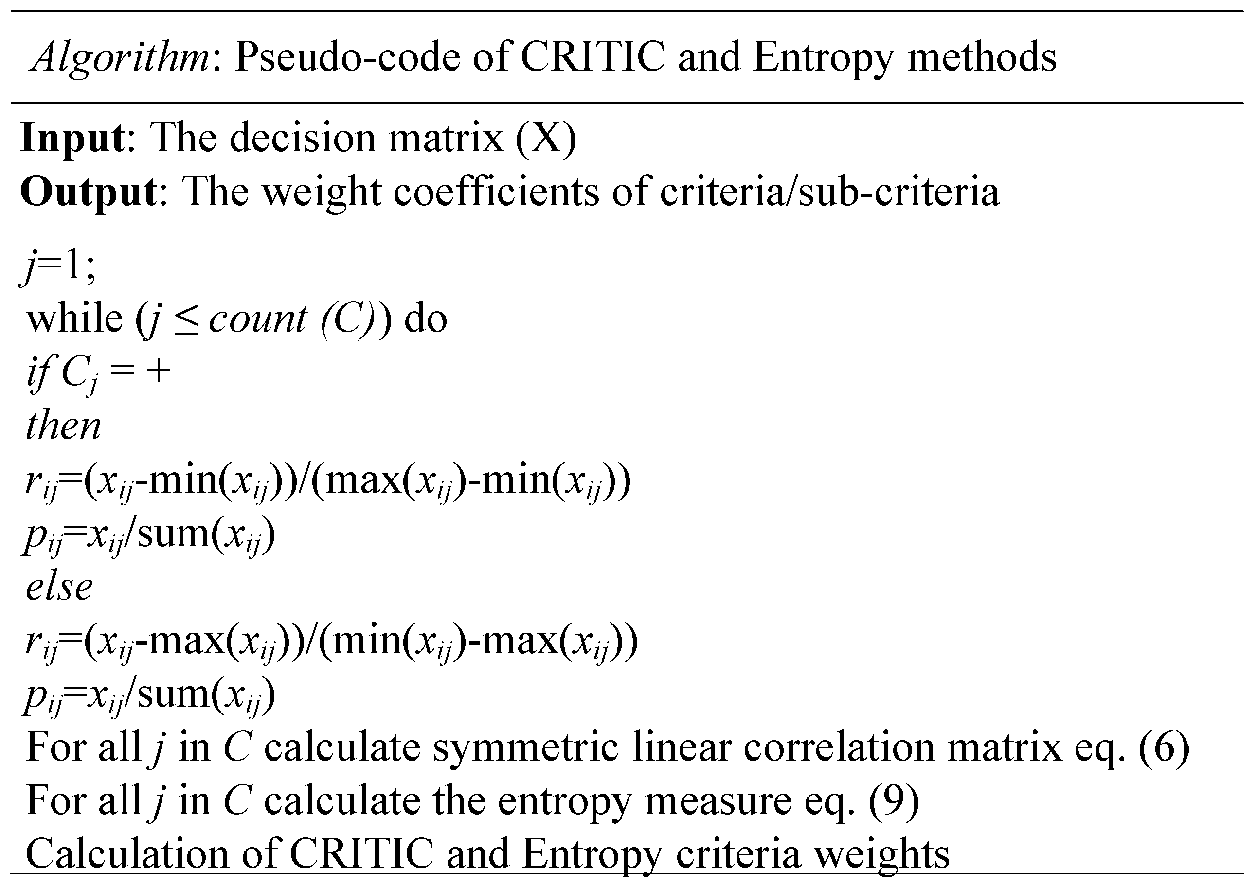
3.3. CRITIC Method
3.4. Entropy Method
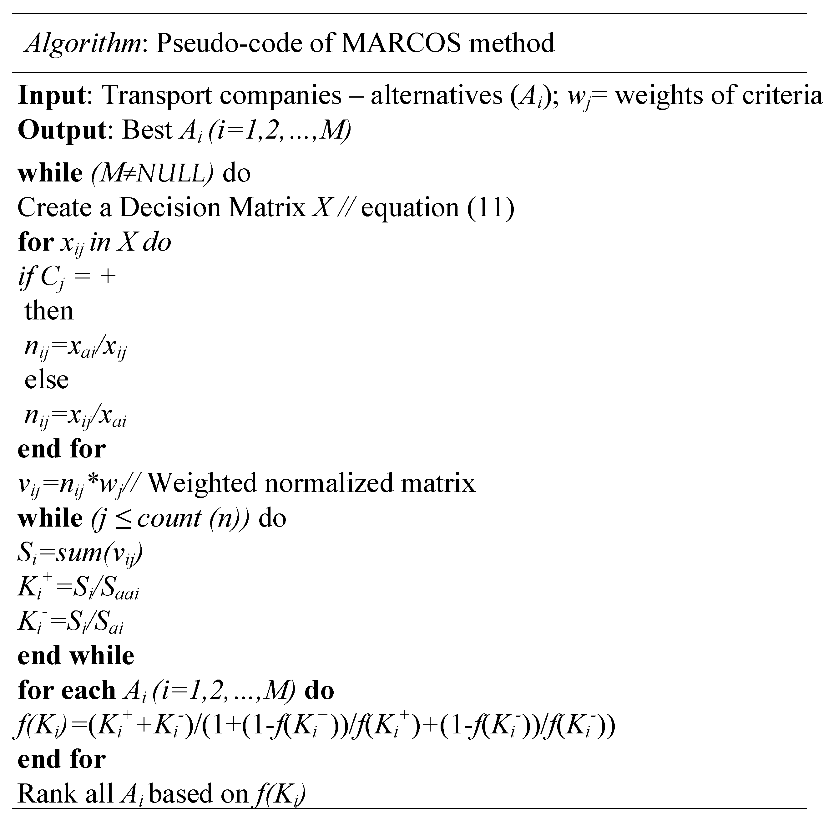
3.5. MARCOS Method
4. Integrated Model for Determining the Efficiency of Transport Companies
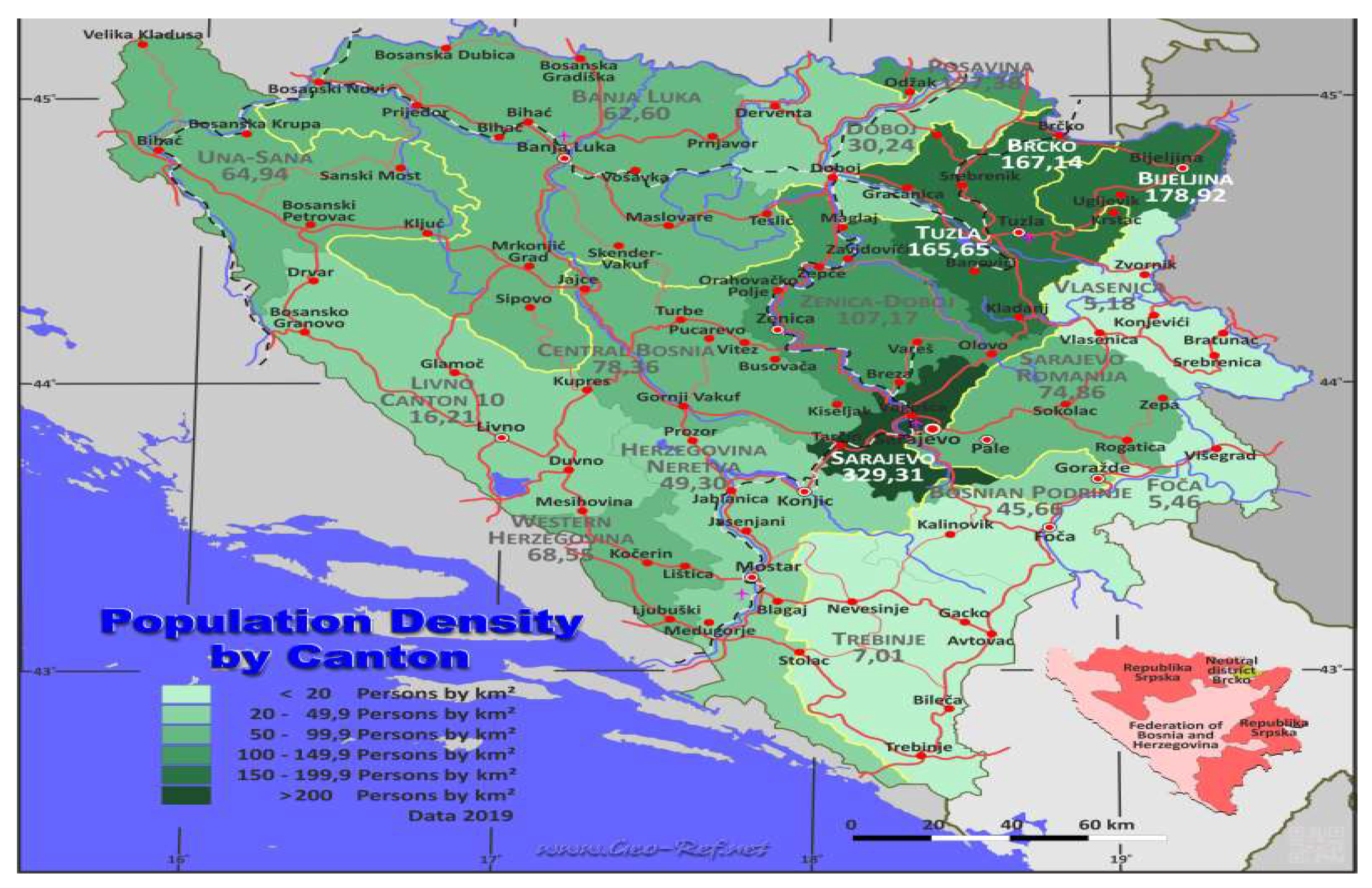
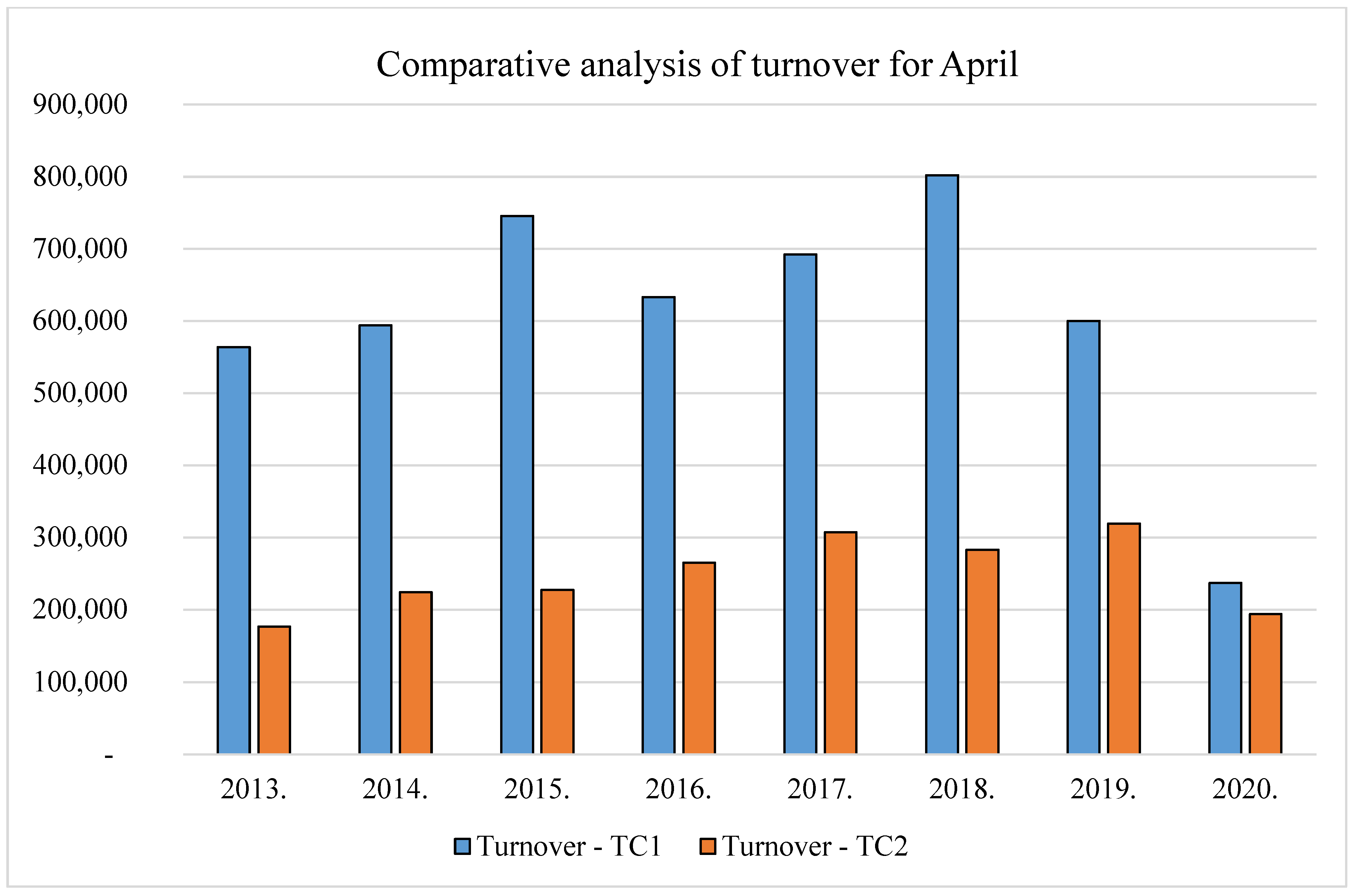
4.1. Analysis of Representative Transport Companies
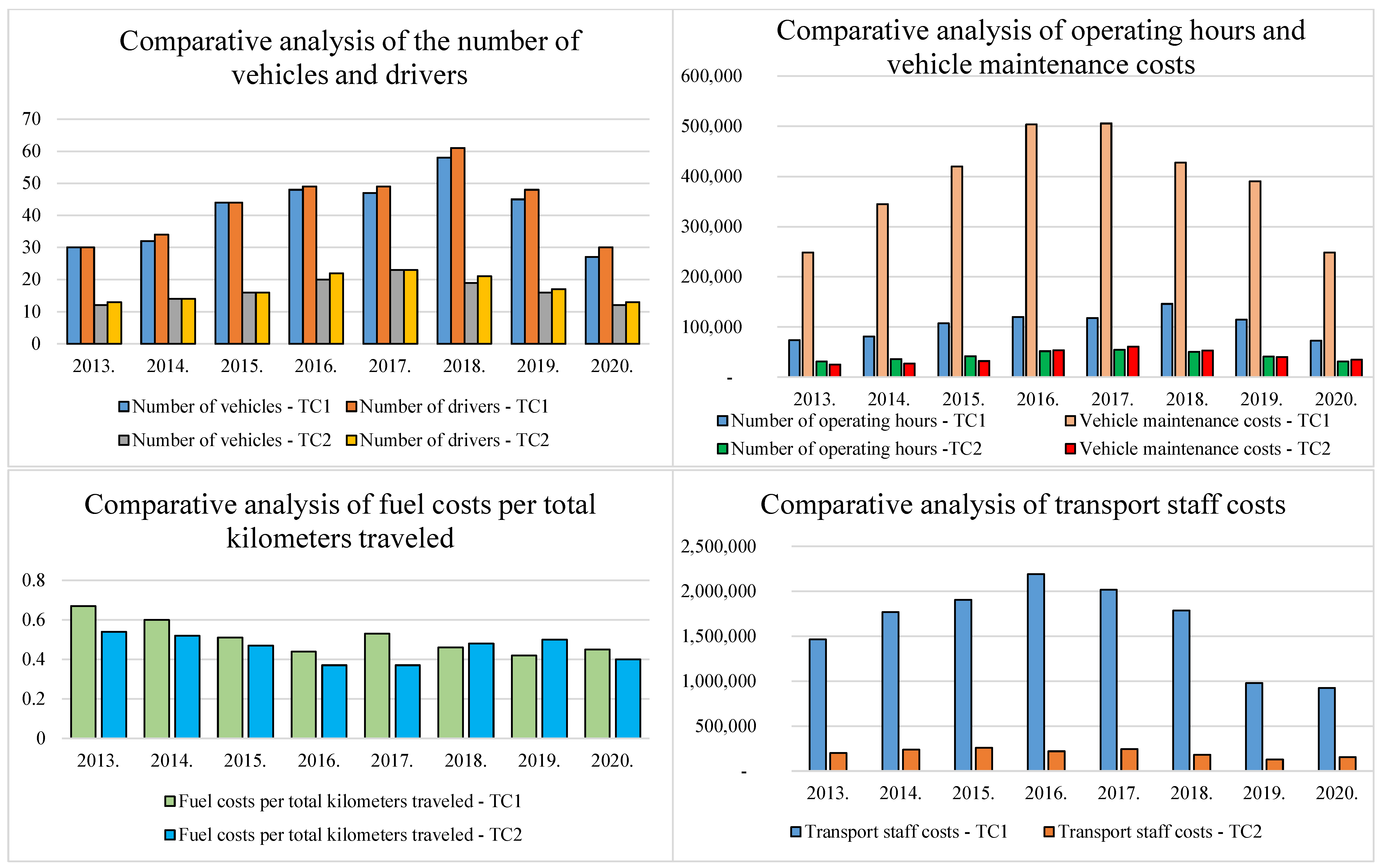
4.2. Data Collections for Inputs and Outputs
4.3. Determining Efficiency Using an Integrated PCA–DEA Model
4.4. Determining the Weight Values of Parameters Applying the CRITIC Method
4.5. Determining the Weight Values of Parameters Applying the Entropy Method
4.6. Ranking the Alternatives Applying the MARCOS Method
5. Sensitivity Analysis and Comparative Analysis
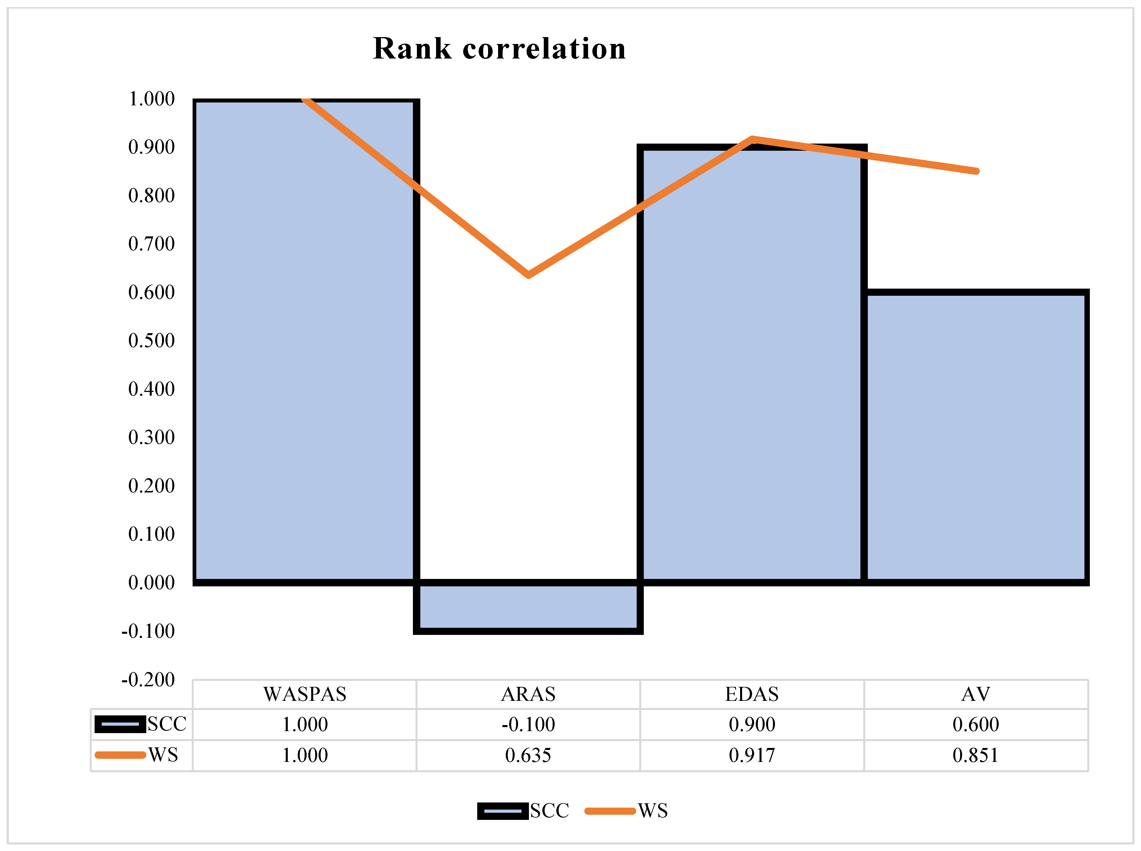
5.1. Comparative Analysis with Other MCDM Methods
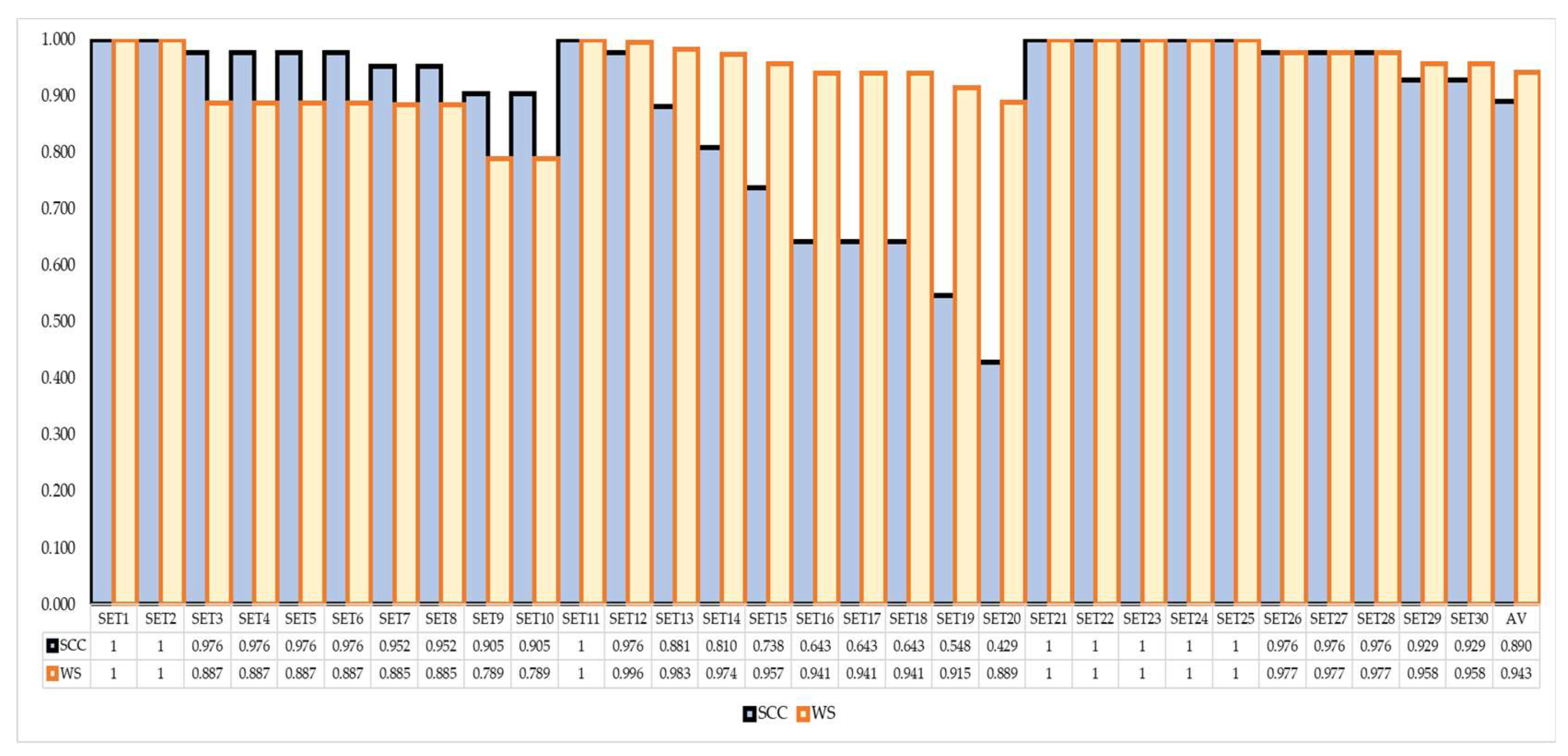
5.2. Changes in Parameter Significance
6. Discussion
6.1. Discussion of Obtained Results
6.2. Discussion Related to Other Studies
6.3. Managerial Implications
7. Conclusions
Author Contributions
Funding
Institutional Review Board Statement
Informed Consent Statement
Data Availability Statement
Conflicts of Interest
References
- Sénquiz-Díaz, C. The Effect of Transport and Logistics on Trade Facilitation and Trade: A PLS-SEM Approach. Economics 2021, 9, 11–24. [Google Scholar] [CrossRef]
- Sénquiz-Díaz, C. Transport infrastructure quality and logistics performance in exports. Economics 2021, 9, 107–124. [Google Scholar] [CrossRef]
- Bugarčić, F.Ž.; Skvarciany, V.; Stanišić, N. Logistics performance index in international trade: Case of Central and Eastern European and Western Balkans countries. Bus. Theory Pract. 2020, 21, 452–459. [Google Scholar] [CrossRef]
- Filová, A.; Hrdá, V. Managerial Evaluation of the Logistics Performance and Its Dependencies on Economies in Selected Countries. Ekon.-Manaz. Spektrum 2021, 15, 15–27. [Google Scholar] [CrossRef]
- Jensen, D.M.; Granzin, K.L. Consumer Logistics: The Transportation Subsystem. In Proceedings of the 1985 Academy of Marketing Science (AMS) Annual Conference; Springer: Cham, Switzerland, 2015; pp. 26–30. [Google Scholar]
- Szymonik, A. Transport Economics for Logistics and Logisticians. Theory and Practice. 2013. Available online: https://www.researchgate.net/publication/297369663_Transport_Economics_for_Logistics_and_Logisticians_Theory_and_Practice (accessed on 10 January 2022).
- Andrejić, M.M. Merenje efikasnosti u logistici. Mil. Tech. Cour. 2013, 61, 84–104. [Google Scholar]
- Ćiraković, L.S.; Bojović, N.J.; Milenković, M.S. Analiza efikasnosti autobuskog podsistema javnog transporta putnika u gradu Beogradu, korišćenjem DEA metode. Tehnika 2014, 69, 1032–1039. [Google Scholar] [CrossRef]
- Dožić, S.; Babić, D. Efikasnost aviokompanija u Evropskoj uniji: Primena AHP i DEA metoda. Proc. Zb. Rad. 2015, V, 512. [Google Scholar]
- Krstić, M.; Tadić, S.; Zečević, S. Analiza efikasnosti evropskih kopnenih trimodalnih terminala efficiency analysis of the European inland trimodal terminals. In Proceedings of the SYMOPIS, Belgrade, Romania, 20–23 September 2020. [Google Scholar]
- Radonjić, A.; Pjevčević, D.; Hrle, Z.; Čolić, V. Application of DEA method to intermodal container transport. Transport 2011, 26, 233–239. [Google Scholar] [CrossRef]
- Karami, S.; Ghasemy Yaghin, R.; Mousazadegan, F. Supplier selection and evaluation in the garment supply chain: An integrated DEA–PCA–VIKOR approach. J. Text. Inst. 2021, 112, 578–595. [Google Scholar] [CrossRef]
- Hatami-Marbini, A.; Hekmat, S.; Agrell, P.J. A strategy-based framework for supplier selection: A grey PCA-DEA approach. Oper. Res. 2020, 22, 263–297. [Google Scholar] [CrossRef]
- Muge, A.K. Exploring the Eco-Efficiency of Transport-Related Particulate Matter Pollution in Nairobi City, Kenya. Open Access Libr. J. 2020, 7, 106279. [Google Scholar] [CrossRef]
- Melo, I.C.; Péra, T.G.; Júnior, P.N.A.; do Nascimento Rebelatto, D.A.; Caixeta-Filho, J.V. Framework for logistics performance index construction using DEA: An application for soybean haulage in Brazil. Transp. Res. Procedia 2020, 48, 3090–3106. [Google Scholar] [CrossRef]
- Ivanović, A.S.; Macura, D.V.; Knežević, N.L. A hybrid model for measuring the efficiency of transport infrastructure projects. Tehnika 2019, 74, 849–857. [Google Scholar] [CrossRef]
- Stević, Ž.; Das, D.K.; Kopić, M. A Novel Multiphase Model for Traffic Safety Evaluation: A Case Study of South Africa. Math. Probl. Eng. 2021, 2021, 5584599. [Google Scholar] [CrossRef]
- Blagojević, A.; Vesković, S.; Stojić, G. DEA model za ocjenu efikasnosti i efektivnosti željezničkih putničkih operatora. Železnice 2019, 2017, 81–94. [Google Scholar]
- Blagojević, A.; Vesković, S.; Kasalica, S.; Gojić, A.; Allamani, A. The application of the fuzzy AHP and DEA for measuring the efficiency of freight transport railway undertakings. Oper. Res. Eng. Sci. Theory Appl. 2020, 3, 1–23. [Google Scholar] [CrossRef]
- Gojić, A. Analiza evropskog tržišta transporta robe i efikasnosti željezničkih operatora. Železnice 2019, 2017, 242–249. [Google Scholar]
- Batur, T.; Nikolić, J. Mjerenje efikasnosti luka i terminala. Naše More Znan. Časopis Za More I Pomor. 2016, 63 (Suppl. 2), 61–64. [Google Scholar]
- Andrejić, M.; Kilibarda, M. Efikasnost logističkih procesa distribucije proizvoda. 2011. Available online: http://www.cqm.rs/2011/FQ2011/pdf/38/37.pdf (accessed on 10 January 2022).
- Kampf, R.; Cejka, J.; Telecky, M. Applicability of the DEA method on the transport undertakings in selected regions. Commun.-Sci. Lett. Univ. Zilina 2016, 18, 129–132. [Google Scholar] [CrossRef]
- Hajduk, S. Efficiency evaluation of urban transport using the DEA method. Equilibrium. Q. J. Econ. Econ. Policy 2018, 13, 141–157. [Google Scholar]
- Azadeh, A.; Salehi, V. Modeling and optimizing efficiency gap between managers and operators in integrated resilient systems: The case of a petrochemical plant. Process Saf. Environ. Prot. 2014, 92, 766–778. [Google Scholar] [CrossRef]
- Davoudabadi, R.; Mousavi, S.M.; Sharifi, E. An integrated weighting and ranking model based on entropy, DEA and PCA considering two aggregation approaches for resilient supplier selection problem. J. Comput. Sci. 2020, 40, 101074. [Google Scholar] [CrossRef]
- Deng, F.; Xu, L.; Fang, Y.; Gong, Q.; Li, Z. PCA-DEA-Tobit regression assessment with carbon emission constraints of China’s logistics industry. J. Clean. Prod. 2020, 271, 122548. [Google Scholar] [CrossRef]
- Layeb, S.B.; Omrane, N.A.; Siala, J.C.; Chaabani, D. Toward a PCA-DEA based Decision Support System: A case study of a third-party logistics provider from Tunisia. In Proceedings of the 2020 4th International Conference on Advanced Systems and Emergent Technologies (IC_ASET), Hammamet, Tunisia, 15–18 December 2020; pp. 294–299. [Google Scholar]
- Andrejić, M.; Kilibarda, M. Distribution channels selection using PCA-DEA approach. Int. J. Traffic Transp. Eng. 2015, 5, 74–81. [Google Scholar] [CrossRef][Green Version]
- Adler, N.; Golany, B. PCA-DEA. In Modeling Data Irregularities and Structural Complexities in Data Envelopment Analysis; Springer: Cham, Switzerland, 2007; pp. 139–153. [Google Scholar]
- Azadeh, A.; Ghaderi, S.F.; Maghsoudi, A. Location optimization of solar plants by an integrated hierarchical DEA PCA approach. Energy Policy 2008, 36, 3993–4004. [Google Scholar] [CrossRef]
- Andrejić, M.M.; Kilibarda, M.J. Measuring global logistics efficiency using PCA-DEA approach. Tehnika 2016, 71, 733–740. [Google Scholar] [CrossRef]
- Wu, H.W.; Zhen, J.; Zhang, J. Urban rail transit operation safety evaluation based on an improved CRITIC method and cloud model. J. Rail Transp. Plan. Manag. 2020, 16, 100206. [Google Scholar] [CrossRef]
- Torkayesh, A.E.; Ecer, F.; Pamucar, D.; Karamaşa, Ç. Comparative assessment of social sustainability performance: Integrated data-driven weighting system and CoCoSo model. Sustain. Cities Soc. 2021, 71, 102975. [Google Scholar] [CrossRef]
- Stević, Ž.; Brković, N. A novel integrated FUCOM-MARCOS model for evaluation of human resources in a transport company. Logistics 2020, 4, 4. [Google Scholar] [CrossRef]
- Biswas, S. Measuring performance of healthcare supply chains in India: A comparative analysis of multi-criteria decision making methods. Decis. Mak. Appl. Manag. Eng. 2020, 3, 162–189. [Google Scholar] [CrossRef]
- Zolfani, S.H.; Bazrafshan, R.; Akaberi, P.; Yazdani, M.; Ecer, F. Combining the suitability-feasibility-acceptability (SFA) strategy with the MCDM approach. Facta Univ. Ser. Mech. Eng. 2021, 19, 579–600. [Google Scholar]
- Ecer, F. A consolidated MCDM framework for performance assessment of battery electric vehicles based on ranking strategies. Renew. Sustain. Energy Rev. 2021, 143, 110916. [Google Scholar] [CrossRef]
- Ecer, F.; Pamucar, D. MARCOS technique under intuitionistic fuzzy environment for determining the COVID-19 pandemic performance of insurance companies in terms of healthcare services. Appl. Soft Comput. 2021, 104, 107199. [Google Scholar] [CrossRef] [PubMed]
- Li, Y.; Yang, J.; Shi, H.; Li, Y. Assessment of sustainable urban transport development based on entropy and unascertained measure. PLoS ONE 2017, 12, e0186893. [Google Scholar]
- Ding, L.; Shao, Z.; Zhang, H.; Xu, C.; Wu, D. A comprehensive evaluation of urban sustainable development in China based on the TOPSIS-entropy method. Sustainability 2016, 8, 746. [Google Scholar] [CrossRef]
- Popović, M. Unapređenje analize obavijanja podataka metodama multiatributivnog odlučivanja: Doktorska disertacija. Универзитет У Беoграду 2019, 1–12. Available online: https://nardus.mpn.gov.rs/handle/123456789/12120 (accessed on 10 January 2022).
- Hlača, B.; Rudić, D.; Kolarić, G. The efficiency of the global transportation system. Zbornik Veleučilišta Rijeci 2015, 3, 160–181. [Google Scholar]
- Pamučar, D.S. Fuzzy-DEA model for measuring the efficiency of transport quality. Vojnotehnički glasnik 2011, 59, 40–61. [Google Scholar] [CrossRef]
- Bašnec, I. Utjecaj COVID-19 na Međunarodnu Trgovinu. Doctoral Dissertation, University North, Koprivnica, Croatia, 2021. [Google Scholar]
- Cui, Q.; He, L.; Liu, Y.; Zheng, Y.; Wei, W.; Yang, B.; Zhou, M. The impacts of COVID-19 pandemic on China’s transport sectors based on the CGE model coupled with a decomposition analysis approach. Transport Policy 2021, 103, 103–115. [Google Scholar] [CrossRef]
- Loske, D. The impact of COVID-19 on transport volume and freight capacity dynamics: An empirical analysis in German food retail logistics. Transp. Res. Interdiscip. Perspect. 2020, 6, 100165. [Google Scholar] [CrossRef]
- Ivanisevic, T.; Simović, S. Dostava robe od strane kurirskih službi, pre i u toku epidemije virusa COVID-19. Put Saobraćaj 2021, 67, 53–56. [Google Scholar] [CrossRef]
- Zhang, J.; Hayashi, Y.; Frank, L.D. COVID-19 and transport: Findings from a world-wide expert survey. Transport Policy 2021, 103, 68–85. [Google Scholar] [CrossRef] [PubMed]
- Jenelius, E.; Cebecauer, M. Impacts of COVID-19 on public transport ridership in Sweden: Analysis of ticket validations, sales and passenger counts. Transp. Res. Interdiscip. Perspect. 2020, 8, 100242. [Google Scholar] [PubMed]
- Arellana, J.; Márquez, L.; Cantillo, V. COVID-19 outbreak in Colombia: An analysis of its impacts on transport systems. J. Adv. Transp. 2020, 2020, 8867316. [Google Scholar] [CrossRef]
- Budd, L.; Ison, S. Responsible Transport: A post-COVID agenda for transport policy and practice. Transp. Res. Interdiscip. Perspect. 2020, 6, 100151. [Google Scholar] [CrossRef] [PubMed]
- Andrejić, M.M. Modeli merenja i unapređenja efikasnosti logističkih procesa distribucije proizvoda. Универзитет у Беoграду 2015, 1–9. Available online: https://nardus.mpn.gov.rs/handle/123456789/4213 (accessed on 10 January 2022).
- Mahmutagić, E.; Stević, Ž.; Nunić, Z.; Chatterjee, P.; Tanackov, I. An integrated decision-making model for efficiency analysis of the forklifts in warehousing systems. Facta Univ. Ser. Mech. Eng. 2021, 19, 537–553. [Google Scholar] [CrossRef]
- Hassanpour, M. An investigation of five generation and regeneration industries using DEA. Oper. Res. Eng. Sci. Theory Appl. 2021, 4, 19–37. [Google Scholar] [CrossRef]
- Bouraima, M.B.; Stević, Ž.; Tanackov, I.; Qiu, Y. Assessing the performance of Sub-Saharan African (SSA) railways based on an integrated Entropy-MARCOS approach. Oper. Res. Eng. Sci. Theory Appl. 2021, 4, 13–35. [Google Scholar] [CrossRef]
- Stević, Ž.; Pamučar, D.; Puška, A.; Chatterjee, P. Sustainable supplier selection in healthcare industries using a new MCDM method: Measurement of alternatives and ranking according to COmpromise solution (MARCOS). Comput. Ind. Eng. 2020, 140, 106231. [Google Scholar] [CrossRef]
- Đalić, I.; Stević, Ž.; Ateljević, J.; Turskis, Z.; Zavadskas, E.K.; Mardani, A. A novel integrated MCDM-SWOT-TOWS model for the strategic decision analysis in transportation company. Facta Univ. Ser. Mech. Eng. 2021, 19, 401–422. [Google Scholar] [CrossRef]
- Sałabun, W.; Urbaniak, K. A new coefficient of rankings similarity in decision-making problems. In Computational Science—ICCS 2020; Springer: Cham, Switzerland, 2020; pp. 632–645. [Google Scholar]
- Kizielewicz, B.; Wątróbski, J.; Sałabun, W. Identification of relevant criteria set in the MCDA process—Wind farm location case study. Energies 2020, 13, 6548. [Google Scholar] [CrossRef]
- Faizi, S.; Sałabun, W.; Nawaz, S.; ur Rehman, A.; Wątróbski, J. Best-Worst method and Hamacher aggregation operations for intuitionistic 2-tuple linguistic sets. Expert Syst. Appl. 2021, 181, 115088. [Google Scholar] [CrossRef]
- Jordá, P.; Cascajo, R.; Monzón, A. Analysis of the Technical Efficiency of Urban Bus Services in Spain Based on SBM Models. ISRN Civ. Eng. 2012, 2012, 984758. [Google Scholar] [CrossRef][Green Version]


| Method | Findings | Observed Inputs and Outputs | Authors |
|---|---|---|---|
| DEA | Analysis of the efficiency of the bus subsystem of public passenger transport | Realized kilometers, realized places/kilometers and number of operationally ready vehicles | Despić et al. [8] |
| AHP and DEA | The analysis of the efficiency of airlines in the European Union | Operational costs, number of employees and offered capacity and realized passenger kilometers | Dožić and Babić [9] |
| DEA | Efficiency analysis of the European inland trimodal terminals | Terminal area, total track length, total operational shore length, maximum draft depth, storage capacity and annual terminal capacity | Krstić et al. [10] |
| DEA | An assessment of intermodal container transportation | The sum of transportation costs, time travel utilization, transportation work and strategy resistance factor | Radonjić et al. [11] |
| DEA, PCA and VIKOR | Supplier selection and evaluation in the garment supply chain | Quality, price, location, lead-time, monetary position (variability), financial position, on-time delivery, ability to produce, support and service and technical capacity | Karami et al. [12] |
| PCA and DEA | Developing A strategy-based framework for supplier selection | Delivery time, service relation combination, cost and organizational management | Hatami-Marbini et al. [13] |
| PCA, DEA and MLR | An assessment of the Eco-Efficiency of Transport-Related Particulate Matter Pollution | Fuel consumption, the number of employees, trips per day, pollution and emissions of various harmful gases | Muge [14] |
| DEA | Research in the new framework for logistics performance index | Freight price, logistic loss, fuel consumption, on-farm storage capacity, emissions (Eq. CO2/transported t), length of the route, production, corridor exports and inverted emission | Melo [15] |
| ANP and DEA | Measuring the efficiency of transport infrastructure projects | 15 inputs/outputs related to energy, quality, operational indicators, utilization and resource indicators | Ivanović et al. [16] |
| DEA, CRITIC and MARCOS | An assessment of Traffic Safety in South Africa | The average number of accidents (per km), the number of access (per km), road width, the number of lanes | Stević et al. [17] |
| Year-DMU | Input Parameters | Output Parameters | ||||||||
|---|---|---|---|---|---|---|---|---|---|---|
| Number of Vehicles | Number of Drivers | Number of Operating Hours | Vehicle Maintenance Costs | Fuel costs Per Kilometers Traveled | Transport Staff Costs | Total Number of Deliveries | Quantity Transported | Kilometers Traveled | Profit | |
| 2013 | 30 | 30 | 74,000 | 248,505 | 0.67 | 1,463,427 | 2931 | 58,620 | 3,000,000 | 328,675 |
| 2014 | 32 | 34 | 81,000 | 344,852 | 0.60 | 1,769,294 | 2917 | 58,340 | 3,700,000 | 217,144 |
| 2015 | 44 | 44 | 107,000 | 419,855 | 0.51 | 1,904,486 | 3611 | 72,220 | 4,224,000 | 302,445 |
| 2016 | 48 | 49 | 119,600 | 503,687 | 0.44 | 2,190,264 | 3672 | 73,440 | 4,704,000 | 309,331 |
| 2017 | 47 | 49 | 117,600 | 505,906 | 0.53 | 2,016,107 | 3930 | 78,600 | 4,900,000 | 313,002 |
| 2018 | 58 | 61 | 146,000 | 427,432 | 0.46 | 1,785,322 | 3849 | 76,980 | 5,856,000 | 148,554 |
| 2019 | 45 | 48 | 115,000 | 390,278 | 0.42 | 981,066 | 3126 | 62,250 | 4,608,000 | 86,743 |
| 2020 | 27 | 30 | 73,000 | 248,505 | 0.45 | 925,000 | 2168 | 43,360 | 2,880,000 | −205,389 |
| Year-DMU | Input Parameters | Output Parameters | ||||||||
|---|---|---|---|---|---|---|---|---|---|---|
| Number of Vehicles | Number of Drivers | Number of Operating Hours | Vehicle Maintenance Costs | Fuel Costs Per kilometers Traveled | Transport Staff Costs | Total Number of Deliveries | Quantity TRANSPORTED | Kilometers Traveled | Profit | |
| 2013 | 12 | 13 | 31,000 | 25,000 | 0.54 | 200,000 | 1741 | 34,800 | 1,150,000 | 97,000 |
| 2014 | 14 | 14 | 36,000 | 27,000 | 0.52 | 240,000 | 2007 | 40,100 | 1,344,000 | 170,000 |
| 2015 | 16 | 16 | 41,500 | 32,000 | 0.47 | 260,000 | 2230 | 44,500 | 1,530,000 | 301,000 |
| 2016 | 20 | 22 | 51,800 | 54,000 | 0.37 | 220,000 | 2744 | 54,000 | 1,920,000 | 319,000 |
| 2017 | 23 | 23 | 55,000 | 61,000 | 0.37 | 245,000 | 2995 | 58,000 | 2,100,000 | 196,000 |
| 2018 | 19 | 21 | 50,400 | 53,000 | 0.48 | 180,000 | 2662 | 53,200 | 1,820,000 | 110,000 |
| 2019 | 16 | 17 | 41,000 | 40,000 | 0.5 | 130,000 | 2214 | 44,000 | 1,500,000 | 12,000 |
| 2020 | 12 | 13 | 31,000 | 35,000 | 0.4 | 155,000 | 1675 | 33,500 | 1,250,000 | 33,000 |
| DEA | PCA–DEA | ||||
|---|---|---|---|---|---|
| 6-4 | 3-3 | 3-2 | 2-2 | 1-1 | |
| DMU1 | 0.966 | 0.942 | 0.756 | 0.609 | 0.593 |
| DMU2 | 1.000 | 1.000 | 0.722 | 0.616 | 0.524 |
| DMU3 | 0.969 | 0.954 | 0.900 | 0.842 | 0.532 |
| DMU4 | 1.000 | 1.000 | 1.000 | 0.953 | 0.496 |
| DMU5 | 1.000 | 1.000 | 0.941 | 0.881 | 0.530 |
| DMU6 | 1.000 | 1.000 | 1.000 | 1.000 | 0.475 |
| DMU7 | 1.000 | 1.000 | 0.936 | 0.935 | 0.485 |
| DMU8 | 0.987 | 0.939 | 0.682 | 0.633 | 0.416 |
| DMU9 | 1.000 | 0.989 | 0.987 | 0.985 | 0.807 |
| DMU10 | 1.000 | 1.000 | 1.000 | 1.000 | 0.888 |
| DMU11 | 1.000 | 1.000 | 1.000 | 1.000 | 0.970 |
| DMU12 | 1.000 | 1.000 | 1.000 | 1.000 | 1.000 |
| DMU13 | 1.000 | 1.000 | 1.000 | 1.000 | 0.950 |
| DMU14 | 1.000 | 1.000 | 1.000 | 0.999 | 0.888 |
| DMU15 | 1.000 | 1.000 | 1.000 | 0.997 | 0.821 |
| DMU16 | 1.000 | 1.000 | 0.980 | 0.980 | 0.817 |
| C1 | C2 | C3 | C4 | C5 | C6 | C7 | C8 | C9 | C10 | |
|---|---|---|---|---|---|---|---|---|---|---|
| Cj | 1.636 | 1.692 | 1.697 | 5.549 | 2.561 | 4.555 | 1.848 | 1.854 | 1.644 | 2.797 |
| wj | 0.063 | 0.065 | 0.066 | 0.215 | 0.099 | 0.176 | 0.072 | 0.072 | 0.064 | 0.108 |
| C1 | C2 | C3 | C4 | C5 | C6 | C7 | C8 | C9 | C10 | |
|---|---|---|---|---|---|---|---|---|---|---|
| Cj | 1.511 | 1.726 | 1.637 | 5.833 | 2.374 | 4.165 | 1.537 | 1.575 | 1.482 | 2.530 |
| wj | 0.062 | 0.071 | 0.067 | 0.239 | 0.097 | 0.171 | 0.063 | 0.065 | 0.061 | 0.104 |
| C1 | C2 | C3 | C4 | C5 | C6 | C7 | C8 | C9 | C10 | |
|---|---|---|---|---|---|---|---|---|---|---|
| TC1 | 0.071 | 0.071 | 0.069 | 0.148 | 0.066 | 0.139 | 0.056 | 0.056 | 0.065 | 0.258 |
| TC2 | 0.057 | 0.061 | 0.056 | 0.170 | 0.059 | 0.110 | 0.052 | 0.051 | 0.052 | 0.332 |
| Both companies | 0.073 | 0.072 | 0.071 | 0.227 | 0.049 | 0.214 | 0.044 | 0.044 | 0.077 | 0.127 |
| Si | Ki− | Ki+ | fK− | fK+ | fKi+ | Rank | |
|---|---|---|---|---|---|---|---|
| AAI | 0.253 | 1.000 | |||||
| DMU6 | 0.590 | 2.336 | 0.590 | 0.202 | 0.798 | 0.5615 | 5 |
| DMU10 | 0.635 | 2.513 | 0.635 | 0.202 | 0.798 | 0.6042 | 3 |
| DMU11 | 0.650 | 2.574 | 0.650 | 0.202 | 0.798 | 0.6187 | 2 |
| DMU12 | 0.656 | 2.595 | 0.656 | 0.202 | 0.798 | 0.6239 | 1 |
| DMU13 | 0.591 | 2.339 | 0.591 | 0.202 | 0.798 | 0.5623 | 4 |
| AI | 1.000 | 1.000 |
| MARCOS | WASPAS | ARAS | EDAS | |||||
|---|---|---|---|---|---|---|---|---|
| fKi | Rank | A | Rank | Ki | Rank | ASi | Rank | |
| DMU6 | 0.562 | 5 | 0.464 | 5 | 0.615 | 1 | 0.500 | 5 |
| DMU10 | 0.604 | 3 | 0.589 | 3 | 0.604 | 4 | 0.734 | 4 |
| DMU11 | 0.619 | 2 | 0.617 | 2 | 0.613 | 2 | 0.770 | 2 |
| DMU12 | 0.624 | 1 | 0.627 | 1 | 0.611 | 3 | 0.792 | 1 |
| DMU13 | 0.562 | 4 | 0.572 | 4 | 0.558 | 5 | 0.740 | 3 |
| Both Companies | |||
|---|---|---|---|
| DMU1 | 0.609 | DMU9 | 0.985 |
| DMU2 | 0.616 | DMU10 | 1.000 |
| DMU3 | 0.842 | DMU11 | 1.000 |
| DMU4 | 0.953 | DMU12 | 1.000 |
| DMU5 | 0.881 | DMU13 | 1.000 |
| DMU6 | 1.000 | DMU14 | 0.999 |
| DMU7 | 0.935 | DMU15 | 0.997 |
| DMU8 | 0.633 | DMU16 | 0.980 |
Publisher’s Note: MDPI stays neutral with regard to jurisdictional claims in published maps and institutional affiliations. |
© 2022 by the authors. Licensee MDPI, Basel, Switzerland. This article is an open access article distributed under the terms and conditions of the Creative Commons Attribution (CC BY) license (https://creativecommons.org/licenses/by/4.0/).
Share and Cite
Stević, Ž.; Miškić, S.; Vojinović, D.; Huskanović, E.; Stanković, M.; Pamučar, D. Development of a Model for Evaluating the Efficiency of Transport Companies: PCA–DEA–MCDM Model. Axioms 2022, 11, 140. https://doi.org/10.3390/axioms11030140
Stević Ž, Miškić S, Vojinović D, Huskanović E, Stanković M, Pamučar D. Development of a Model for Evaluating the Efficiency of Transport Companies: PCA–DEA–MCDM Model. Axioms. 2022; 11(3):140. https://doi.org/10.3390/axioms11030140
Chicago/Turabian StyleStević, Željko, Smiljka Miškić, Dragan Vojinović, Eldina Huskanović, Miomir Stanković, and Dragan Pamučar. 2022. "Development of a Model for Evaluating the Efficiency of Transport Companies: PCA–DEA–MCDM Model" Axioms 11, no. 3: 140. https://doi.org/10.3390/axioms11030140
APA StyleStević, Ž., Miškić, S., Vojinović, D., Huskanović, E., Stanković, M., & Pamučar, D. (2022). Development of a Model for Evaluating the Efficiency of Transport Companies: PCA–DEA–MCDM Model. Axioms, 11(3), 140. https://doi.org/10.3390/axioms11030140