1. Introduction
The main goal of this paper is to determine the required number of exploratory wells for additional landslides for different types of landslides, and methods used for their remediation, using the method of multicriteria optimization (PROMETHEE), taking into account the effects of increasing workloads, which can greatly affect the total costs of landslide remediation and which may lead to exceeding the planned budget.
The article is organized as follows.
Section 2 points out the importance of applying multicriteria optimization methods in solving landslide remediation problems and lists the most commonly used methods. For the purposes of research in this paper, the PROMETHEE method was chosen and the theoretical foundations on which it is based are presented.
In
Section 3, case studies on the examples of seven landslides located in the territory of the Republic of Serbia are presented, in order to consider a wide range of effects of multicriteria optimization of the application of the PROMETHEE method. Activities, criteria, and appropriate weighting coefficients are defined. For the given scenarios (and selected preferences) and based on the ranking of the flow function, the function of the number of wells was optimized during additional soil subsidence. The obtained results are presented and a comment is made on the obtained ranking results.
Sensitivity analysis of the obtained results was performed. For sensitivity analysis, in addition to the given criteria, data were used to increase the amount of material ΔV of the performed state of landslide remediation Vi according to the amount of material of the project solution of landslide remediation
In
Section 4, the corresponding conclusions are derived from the multicriteria method of optimization of the given problem presented in the previous section.
Section 5 describes the contribution of the work to science.
Estimating the condition of the landslide and the need for remediation of the same representation is a complex engineering-technological-economic problem that is solved by analyzing several parameters in the process of making the final decision. In the preliminary phase of the project development, the methods of remediation are considered, taking into account the engineering (rehabilitation technology, change in the geometry of the section, the system of drains, different types of support structures, application of deep foundation (piles) in combination with other geotechnical structures, application of coatings, application geosynthetics, geo and geochemicals, injection of masses of soil, application of electro osmosis, etc.) and economic (work premise and calculations) aspects of rehabilitation. The final design solution implies the selection of an optimal remediation method with the appropriate safety factor.
One of the most important aspects in landslide remediation, in addition to the analysis of landslide stability, is the problem of estimating the quantity of earthworks. When landscaping the landslide, situations arise such that, when excavated, the influence of destabilizing forces is further increased, which was not originally taken into account. The soil that forms the slopes of the excavation plays a role in secondary landslides that may or may not have to be activated. In the case of activation, an additional quantity of earth is being ruined, increasing the effect of the existing landslide. Experience in practice so far has shown that if these soil erosion effects are not taken into account at the stage of development of project documentation, the cost of rehabilitation can be up to 20% higher. In certain situations, this percentage increase may be even higher.
For a mass of soil that collapses during the rehabilitation of the main landslide, additional research and analyses are carried out (length of landslide and number of boreholes with increase of excavation and embankment, surface of landslide, number of boreholes per hectare with increase of excavation and embankment, drilling per hectare with increase of excavation and embankments, cost of drilling with projected price, and cost of drilling costs with the cost of execution). The big problem for the investor is the number of exploration wells, since the increase in the number of wells also increases the cost of landslide remediation. The cost of geomechanical exploration increases, and therefore the cost of the project. Determining the safety factor requires more detailed input parameters, which are directly correlated with the number of exploratory wells.
2. Application of Multi-Criteria Optimization to Landslide Rehabilitation
Solving such problems can be achieved through the application of multi-criteria optimization methods (MCDM—Multi-Criteria Decision Making). Multi-criteria optimization of landslide remediation is considered through the function of the amount of work in the additional soil erosion. Using multi-criteria optimization in the analysis of landslides with additional soil erosion can emphasize the good and bad aspects of the landslide removal method itself [
1,
2].
Today there is a considerable number of multi-criteria optimization methods in which the solution of a multi-criteria problem is obtained by choosing the best alternative from a set of defined alternatives (MADM—Multi-Attribute Decision Making) or by programming the best alternative (MODM—Multi-Objective Decision Making). The most commonly used methods are TOPSIS [
3,
4], VIKOR, ELECTRE [
5,
6,
7,
8,
9], PROMETHEE, etc.
For the purposes of this research, the PROMETHEE method was selected, given its proven reliability in the application of various multi-criteria problems in different engineering and economic fields. The key elements of PROMETHEE methods are predefined scenarios, activities, criteria, and appropriate weighting coefficient ranking; its interaction provides a spectrum of results that can be used in making final conclusions and decisions for the following facts.
PROMETHEE Method
In general, the mathematical problem according to the PROMETHEE method can be formulated as [
10,
11,
12,
13,
14,
15,
16,
17]:
where
A is the final set of
n activity,
fk are the criteria,
fj(
a) is an evaluation of the activity
a for the given criterion
fj presented in
Table 1.
In the phase of setting the problem and defining the activities and criteria, it is necessary to define the functions of preference and weight coefficients. The preference function for the given criterion and the corresponding set of activity evaluations defines the distribution model and the corresponding intervals of minimum and maximum values. The previously performed statistical data analysis and the qualitative evaluation of the obtained relations of activities and criteria determine the values of the indifference and prevalence interval. Indifference is the largest deviation, the below values are not taken into consideration as minor, while preference represents a slightest deviation taken as sufficient to generate complete preference (crucial in decision making). In general, the preference function can be presented as:
Figure 1 shows the types of preference functions implemented in the PROMETHEE method, for
f(
a) >
f(
b) are [
10,
11,
12,
13,
14,
15,
16,
17]:
Based on the weight coefficients
wi assigned to each criterion, a preference index can be determined:
where it is
If (it is)
π(
a,
b) = 0, then all values are
Pj(
a,
b) = 0, and if (it is)
π(
a,
b) = 1, then all values are
Pj(
a,
b) = 1. Now, for each activity, positive
Φ+ and negative
Φ− flows can be determined:
Rankings based on the usage of
Φ+ and
Φ− flows are partial rankings, while complete ranking is performed according to the term:
A positive flow of preferences shows the degree of importance (dominance) of one activity in relation to other activities, so if the value of the positive flow is greater Φ+→1, then the activity is even more significant. The negative flow of preference indicates the weakness of the activity, or shows how much other activities are preferred in relation to the activity for which (it is) Φ−→0.
3. Case Study
In the case study [
18,
19,
20,
21,
22] on real examples of landslides in the territory of the Republic of Serbia, the multicriteria optimization of landslide landscaping carried out for the budget model is presented—a determination of the required number of boreholes for additional soil erosion.
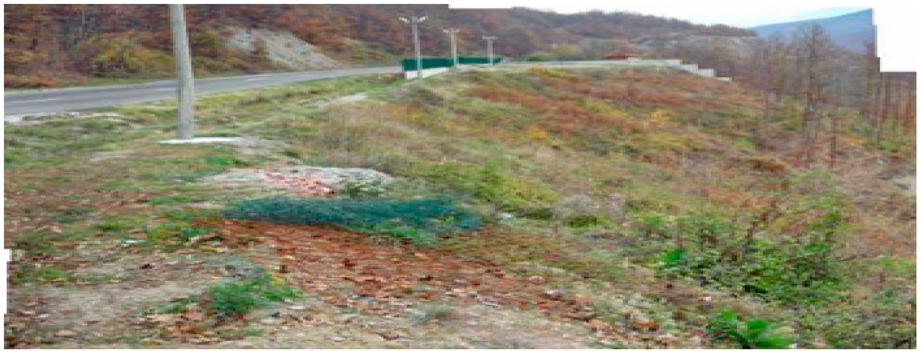
3.1. Kominje
At the site “Kominje 2” (
Figure 2) on the main road M22, the section Novi Pazar—Ribariće km 478 + 910 (ID 0253), due to the terrain slipping, had a road embankment collapse as well as a significant carriageway collapse (on the longitudinal profile of 30 cm length) at a road stretch of 50 m [
23]. The slopes are of elongated shape (the length of the body of the landslide is 50 m and the total height difference is 20 m) and it is made of clay and crushed material by which one erosion groove is filled, and the movement of the material itself is slow and takes place in the form of a phase of intermittent plastic deformations. On steep slope sides, kinematic conditions met with the orientation of the elements of the assembly; deep, blocky landslides or slopes are often formed. The sliding surface is formed in contact with less degraded wall mass.
The project includes a part of the landslide in the traffic zone. First, stability analyses were carried out prior to the planned remediation measures and the position of the critical slip surface was determined with a minimum safety factor in relation to the state of the boundary equilibrium Fs = 1.02. After these conducted analyses, a check of the stability of the slope under the conditions of the designed rehabilitation measures of the newly projected deep trenches D1 and D2 was made, including lowering of groundwater level, drainage, and regulation of surface atmospheric waters. The results of the analysis show that the safety factor obtained is Fs = 1.343. Then, the analysis of the slope stability was carried out under the conditions of the planned remediation measures, including the impact of the earthquake with the coefficient of seismicity K = 0.05. The results of the analysis show that the safety factor obtained is Fs = 1.18.
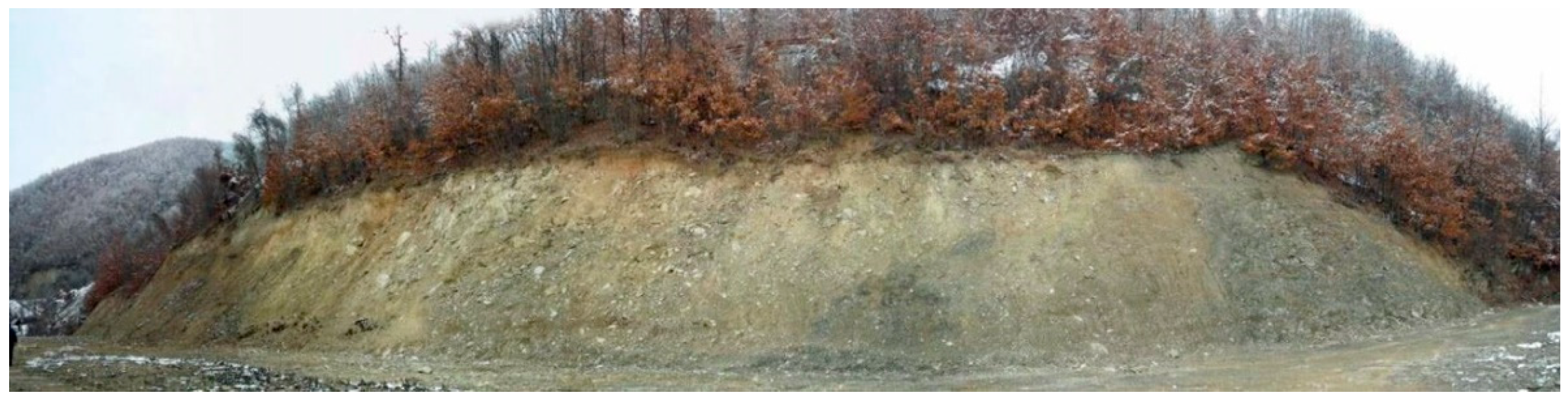
3.2. Zavlaka
On the section of the state road IIA-137 (R-221a) Šabac-Tekeriš-Zavlaka at km 10 + 225, there was a landslide [
24] (
Figure 3). The rehabilitation road route is side out and the destruction involved the left side of the road, the embankment slope. The frontal width of the landslide was 50 m. The activation of the landslide was, due to the sudden drowning of the soil with water and intense swelling of water in the field, as well as the large amount of atmospheric precipitation.
The implemented remedial measures—the drainage system development and the surface regulation of atmospheric waters. Appropriate analyses of the stability of the slopes at the moment of slipping and after the implemented remediation measures were carried out. The analysis of the slope stability was made using the method Morgenstern-Price with the conventionally assumption of the sine function of the inclination of inter-cellular forces. After the development of the longitudinal drainage trench D1 and the cross-drain trench D2, a new stability analysis was performed. The results of the analysis show that the safety factor was Fs = 1.40.
3.3. Jezgroviće
At the “Jezgroviće 2” (
Figure 4) locality of the main M2 road, the Ribariće-Vitkovići section, a 1185 + 100 (ID 0066) km, road route is side cut and the slipping terrain led to the carriageway depression (collapse) at the road stretch of 120 m [
25]. Large cracks and denivelations of 30 cm appeared on carriageway. Some sections of the existing supporting wall were separated and inclined. Traces of rupture separating individual structural blocks of massifs, partially visible on the ground and partly assumed, formed kinematic active fields.
The implemented remediation measures were also adopted—moving one track of the road to the hill, making a reinforced concrete wall and regulation of atmospheric and underground waters. For the characteristic geotechnical profile of the terrain, stability analyses were first performed prior to the planned remediation measures. On the basis of the computational analysis, the position of the critical sliding surface has been determined with a minimum safety factor in relation to the state of the boundary equilibrium, whereby a safety factor Fs = 1.055. The stability of embankments has been examined for the case when the slope is side cut and intersects with a supporting structure Fs = 1.48.
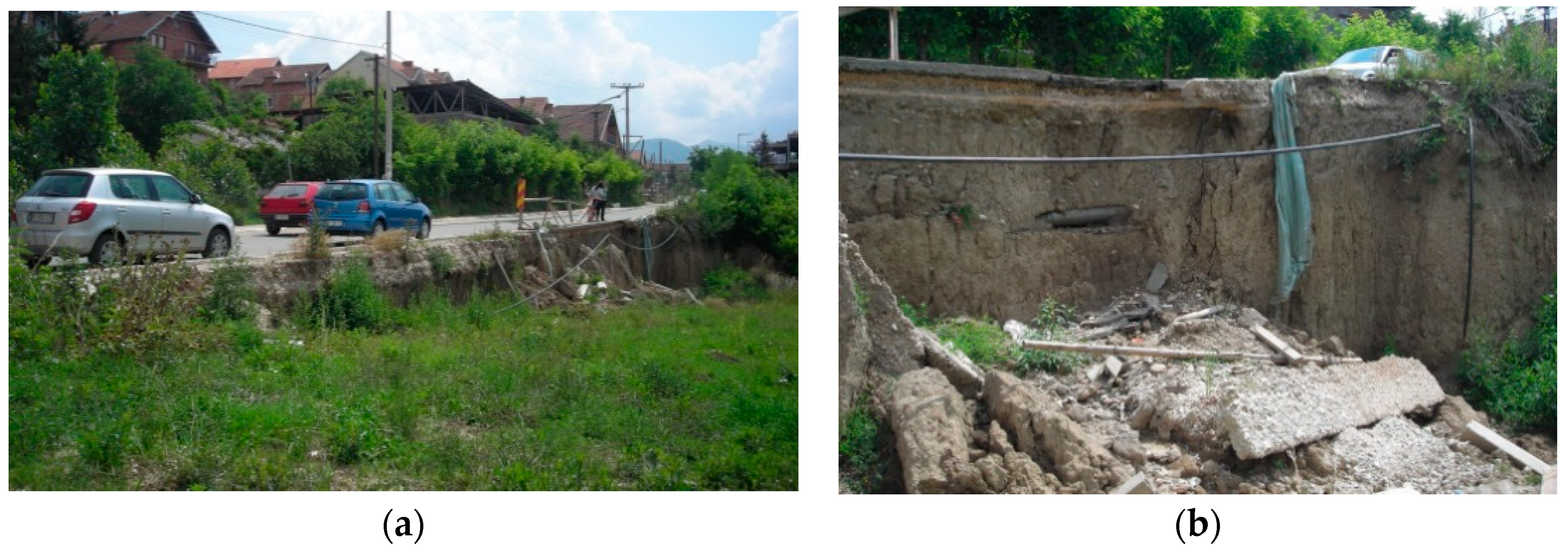
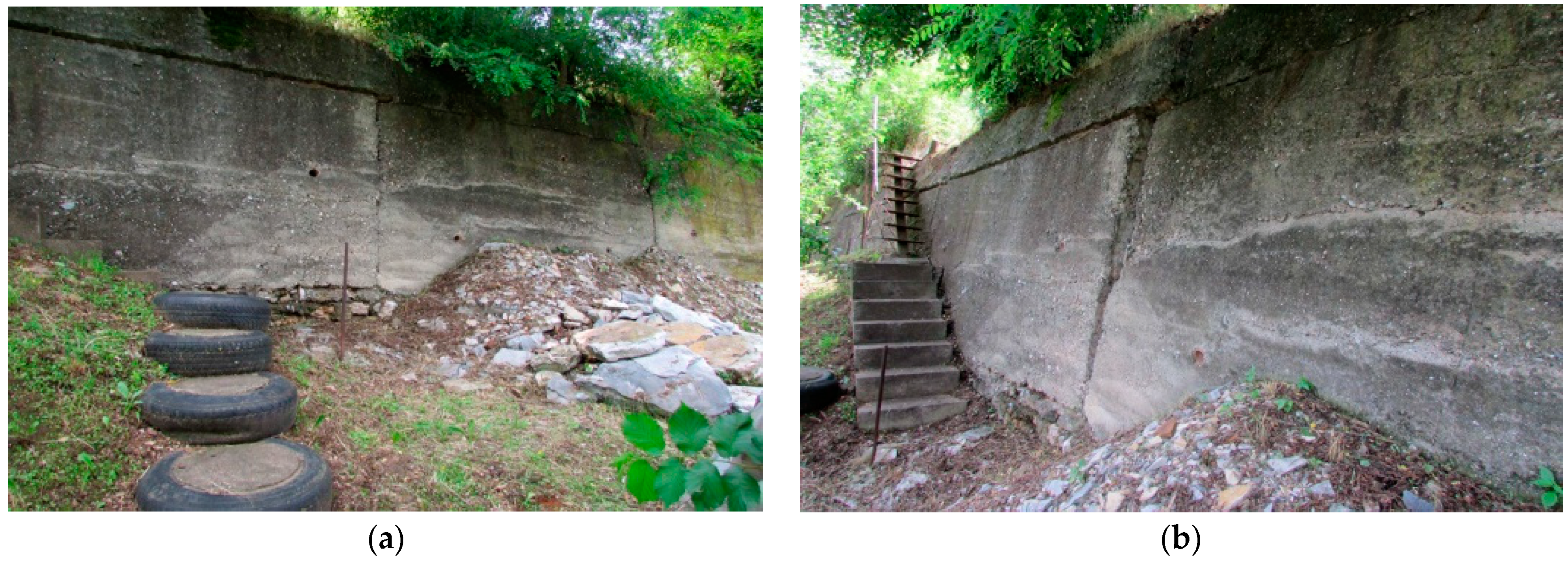
3.4. Footwear Factory
On the part of the regional road II of the line R234, Novi Pazar-Rajetiće (
Figure 5), km 1 + 000, (ID 1086), at the site of the footwear factory (Ruđera Bošković street in Novi Pazar), excavation in the pier from the embankment sheath caused the collapse of the shoulder and part of the pavement [
26]. To plan the plot on the right side of the road, an excavation of a steep cliff was made. After the precipitation and under the load of the road there was a collapse of the mentioned scarp.
The adopted and implemented recovery solution wasthe development of a reinforced concrete wall and regulation of rain and underground water. The first model analyzed the case of a non-concealed slope after excavation. The method of reverse analysis was to examine to what extent the shear strength of the soil was mobilized. The obtained result is valid when groundwater filtration takes place in the field. When a rise in groundwater level in the field forms a line of scattering due to the increase in the pore pressure in the soil, at the expense of effective strength, the slope hits the state of the boundary balance and breakdown (Fs = 0.996). After these conducted analyses, a check of the stability of the slope was achieved in the conditions of the designed rehabilitation measures, i.e., the construction of a reinforced concrete wall, and the safety factor is Fs = 2.194.
3.5. 6 + 900
On the part of the state road IIA-137 (R-127), the section Krupanj-Mačkov Kamen, km 6 + 900, due to heavy precipitation, an active landslide was formed [
27] (
Figure 6). Slipping completely destroyed the hull of the road at the length of 60 m with a leading scar of height of 3–5 m. The length of the landslide is 140 m along the local road and about 50 m below the local road with visible traces of the picking of the fine material from the formed sliding body. In addition to the above-mentioned sliding body, two more sliding bodies were registered in the direction of the growth of the station to Mačkov Kamen. The total width of all three slopes formed on the hill side is 160 m, 60 m of which are interrupted, 100 m along on the slope below the route. At a minimum distance of 5 m below the bank road, the scar was formed at a length of 15 m with a sub vertical denivelations of 8 m.
The adopted and implemented remediation measures are construction of a stone threshold as a support to the new embankment, regulation of underground water (construction of longitudinal drainage on the left side of the road), replacement of a part of the embankments on the right side of the road, regulation of atmospheric waters and protection of the slope from erosion. First, stability analyses were carried out prior to the planned remediation measures; the position of critical sliding surfaces with a minimum safety factor was determined in relation to the state of the boundary equilibrium Fs = 1.001. After this analysis, a check of slope stability was carried out under the conditions of the planned measures for remediation of the newly projected drain, riparian drainage, lowering the level of groundwater, replacing part of the roadway as well as regulating surface waters. The results of the analysis show that the safety factor is Fs = 1.541.
3.6. Pejčina Krivina
At the site “Pejčina krivina”, on the part of the state road IB-23 Požega-Čačak, a slipway was formed [
28] (
Figure 7). The rehabilitation road route is side cut, and the right slope of the embankment road was hit by demolition, in the direction of the growth of the station and the shoulder and about half of the right-hand carriageway. The frontal width of the landslide is 25 m. According to the mechanical properties, the “Pejčina krivine” landslide belongs to the consecutive type of landslide with the tendency of regressive process development.
Remedial measures were adopted and implemented, making a supporting wall to the right edge of the road, a drainage fill behind the wall, regulating atmospheric underground water. Stability analyses were conducted for geotechnical and hydrogeological conditions that led to the occurrence of slip as well as conditions that correspond to the condition after the planned remediation measures. The analyzed cases show that in the period of hydrological extremes, when it is possible to increase the level of groundwater in the field, or when a line of scattering is formed on the slope to a certain height, due to the increase in the pore pressure in the soil, at the expense of effective strength, the slope can reach the state of the boundary balance. After these conducted analyses, the stability of the slope was achieved under the conditions of the planned remediation measures by constructing a supporting structure (supporting wall), lowering the groundwater level as well as collecting surface atmospheric waters. The results of the analysis show that the safety factor is higher than necessary, Fs = 1.368.
3.7. Lubnica
On the R-261 road from Zaječar to Boljevac at km 6 + 412.70 to km 6 + 540.30, at the toponyms “Lubnica”, the already existing landslide was reactivated [
29] (
Figure 8). The landslide is 80 m long and 130 m wide and cover about 1.0 hectare. It is estimated that a wall mass of about 50,000 m
3 is being launched.
To save the slope and put the road into a stable condition, several rehabilitation measures were implemented: posting a new one, quality, sandy-pebbly floor with “mattress” or stone crumbs, drainage system development (longitudinal and transverse drainage trenches), surface water collection by a concrete open channel, and the humidation of the surface of the slope of the road and surface of the landslide whose soil has been replaced.
For shorter active sliding layers, (their length is about 55 m), in high groundwater, a safety factor is obtained FS = 1.15. After making a drainage layer, or by lowering the groundwater for 4–5 m, a safety factor FS = 1.51.
3.8. Application of PROMETHEE Method—Optimization of the Number of Wells in Additional Soil Erosion
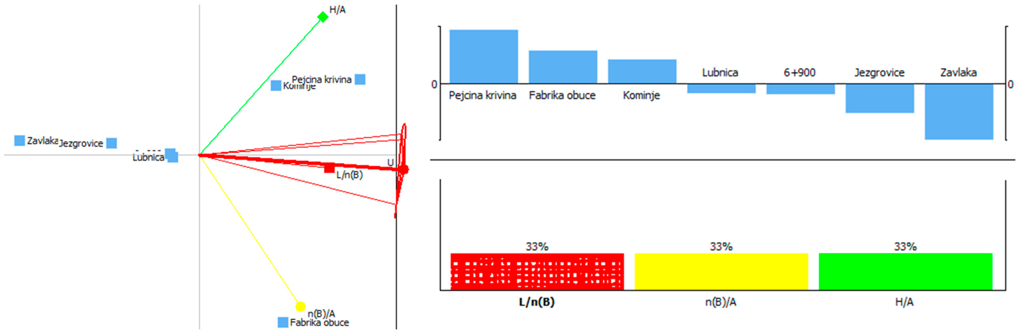
The optimization solutions for the selected number of scenarios are presented in the function of the flow rate
Φ(
a) of the complete ranking. Based on the PROMETHEE ranking, the activities and criteria are presented integrally at the GAIA level [
30]. Here, an agreement or conflict can be established between the criteria, degree of superiority or inferiority of one activity, in relation to other activities. The final solution, according to the GAIA level, is presented using a decision vector that has a defined direction, direction, and intensity and which clearly indicates the position of optimal activity and key criterion.
Optimization Consideration Activities—models of applied landslide remediation with additional soil erosion (7 cases from practice) are:
a1—“Kominje”,
a2—“Zavlaka”,
a3—“Jezgroviće”,
a4—“Footwear factory”,
a5—“6 + 900”,
a6—“Pejčina krivina”,
a7—“Lubnica”.
Optimization Consideration Criteria—The economic effects resulting from quantitative borehole analysis in the additional soil erosion (3 criteria) are [
31]:
C1—the ratio of the landslide length (along the road) and the number of wells L/n(B),
C2—the ratio of the number of wells and surface of the landslide n(B)/A,
C3—the ratio of the amount of drilling over the surface of the landslide H/A.
Scenarios in optimization considerations—basic and combined models of weight coefficient scenarios resulting from quantitative wells analysis in additional soil erosion (seven scenarios) are:
S1—minimization (for min. preference) of the ratio of the length of the landslide (by road) and the number of wells L/n(B),
S2—maximization (for min. preference) of the length of the landslide (by road) and the number of wells L/n(B),
S3—Maximization of (for preference max) ratio of the number of wells and the surface of the landslide n(B)/A,
S4—minimization of (for preference max) ratio of the number of wells and the surface of the landslide n(B)/A,
S5—Maximization of (for preference max) ratio of the quantity of drilling the surface of the landslide H/A,
S6—minimization (for preference max) ratio of the quantity of drilling the surface of the landslide H/A,
S7—combined scenario with equivalent weight coefficients.
The selection of activities was carried out on the basis of the defined landslide relief problem, while the selection of the criteria was based on the conducted economic analysis and the developed economic effects arising from the quantitative analysis of the wells in the additional soil erosion. The matrix relation of activity
a and criteria
c for optimization is shown in
Table 2.
The selection of scenarios, as basic and combined models of weight coefficient scenarios, was carried out in order to examine a wide spectrum of the effects of multi-criteria optimization, in the function of applied models, landscaping landslides and number of wells in additional soil erosion. The matrix of the scenario
S and weight coefficients
w for optimization is shown in
Table 3.
In the case of scenario
S1—the smallest number of wells (minimization (for min. Preference) of the relationship between the length of the landslide (by road) and the number of wells
L/
n(
B)) was realized for the slopes “Kominja” with
Φ = 0.279 (
Figure 9).
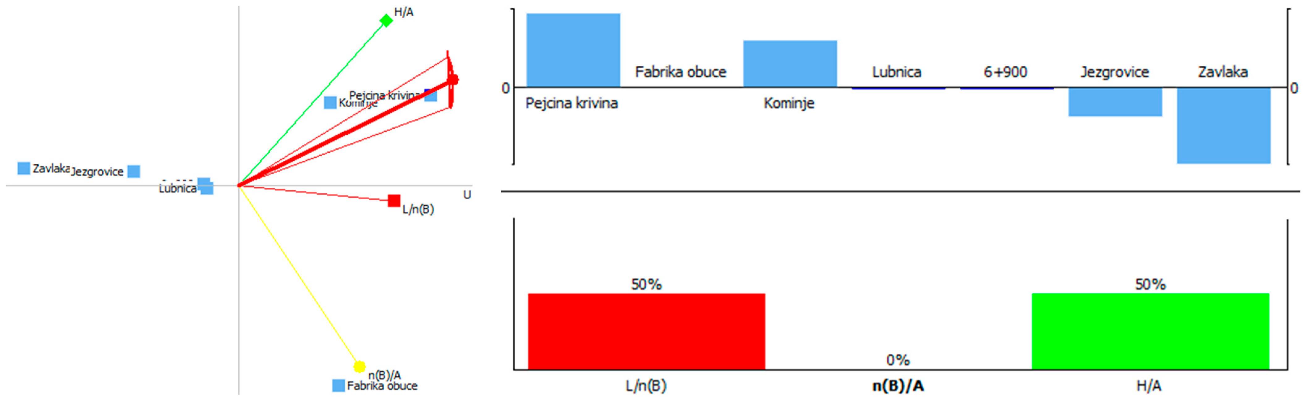
In the case of scenario
S2—maximization (for min. preference) of the length of the landslide (by road) and the number of wells
L/
n(
B) was realized for the slopes “Pejčina krivina” with
Φ = 0.545 (
Figure 10).
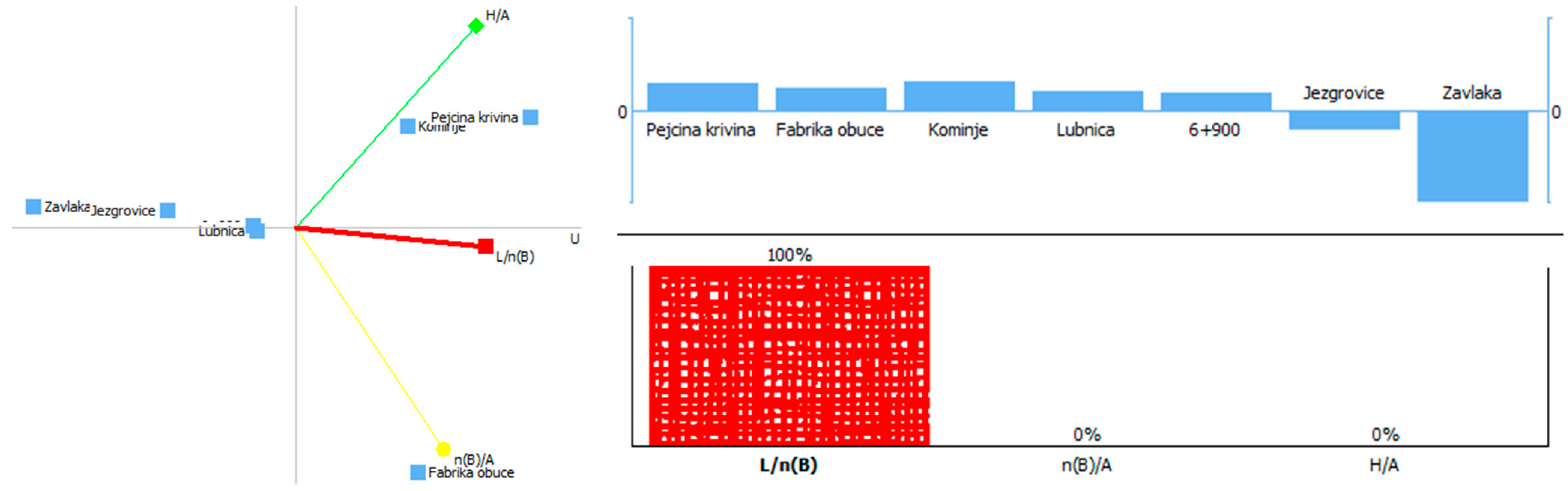
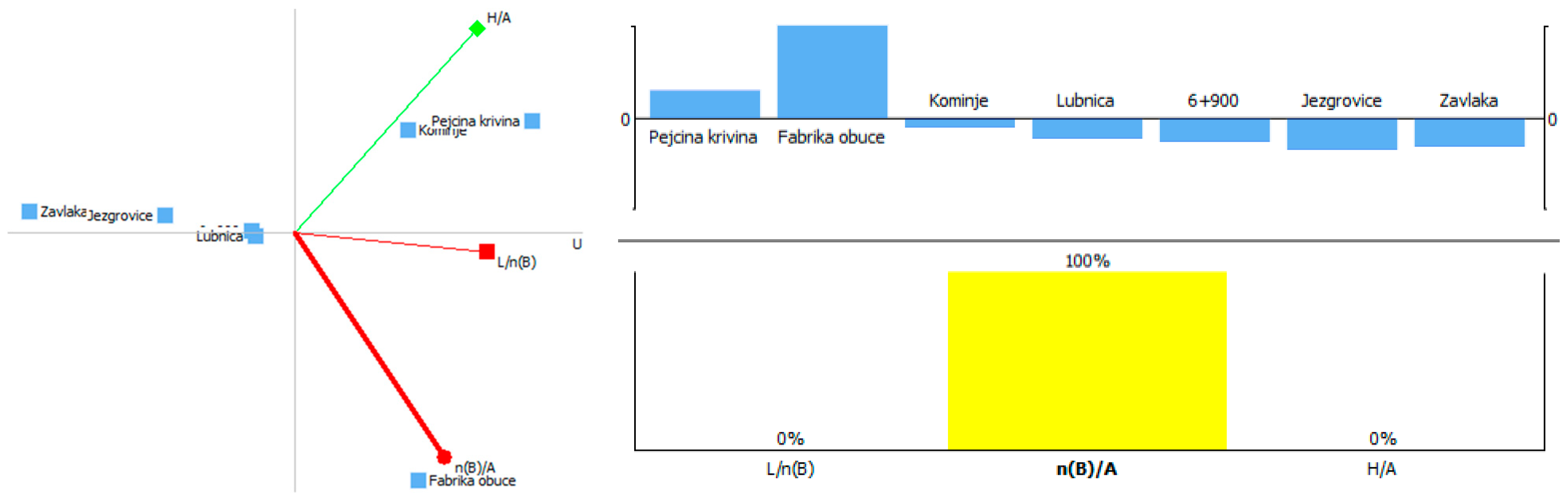
In the case of scenario
S3—Maximization of (for preference max) ratio of the number of wells and the surface of the landslide
n(
B)/
A was realized for the slopes “Footwear Factory”
Φ = 0.859 (
Figure 11).
In the case of scenario
S4—minimization of (for preference max) ratio of the number of wells and the surface of the landslide
n(
B)/
A was realized for the slopes “Pejčina krivina” with
Φ = 0.545 (
Figure 12).
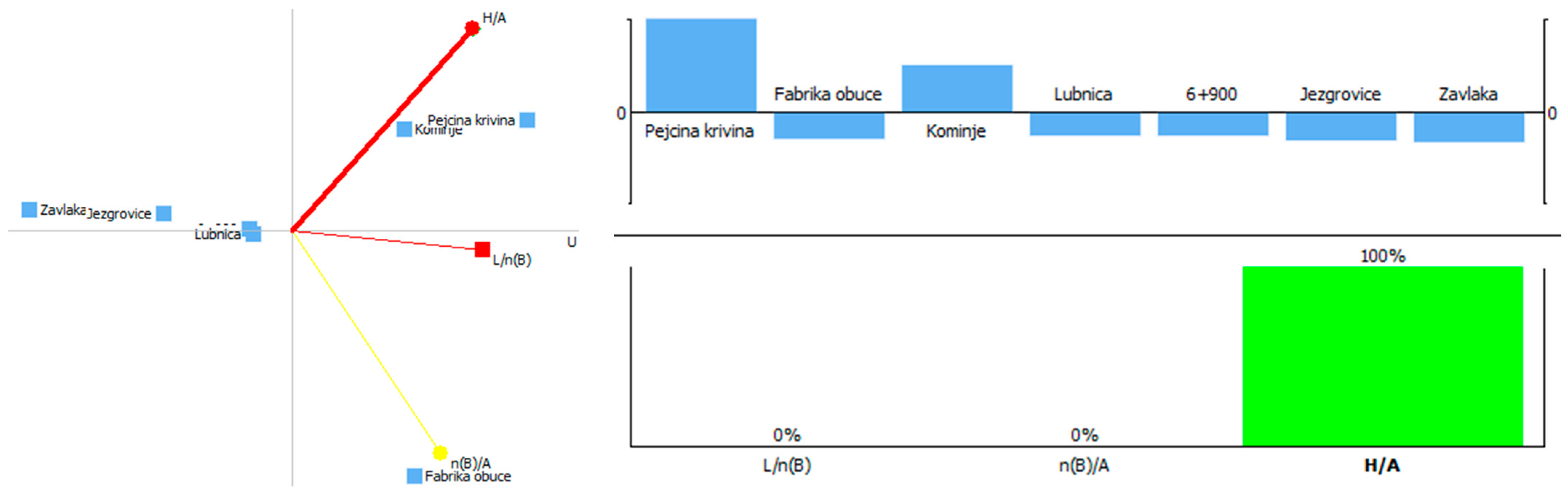
In the case of scenario
S5—Maximization of (for preference max) ratio of the quantity of drilling the surface of the landslide
H/
A was realized for the slopes “Pejčina krivina” with
Φ = 0.839 (
Figure 13).
In the case of scenario
S6—minimization (for preference max) ratio of the quantity of drilling the surface of the landslide
H/
A was realized for the slopes “Footwear factory” with
Φ = 0.535 (
Figure 14).
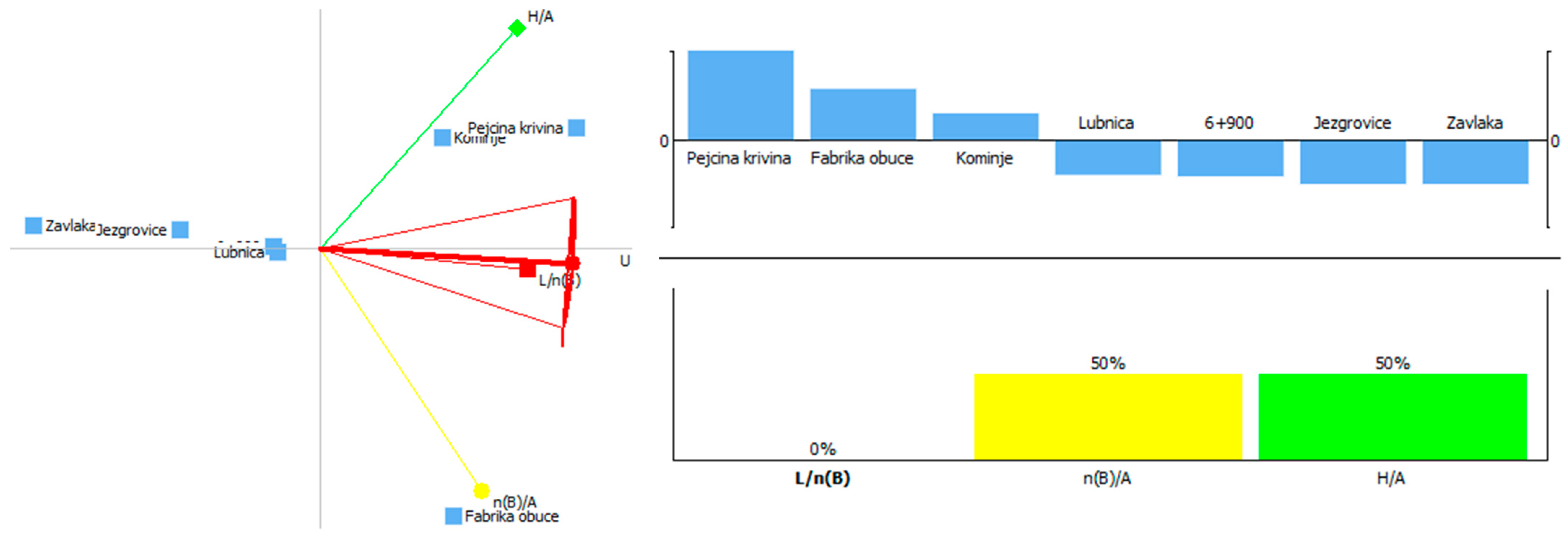
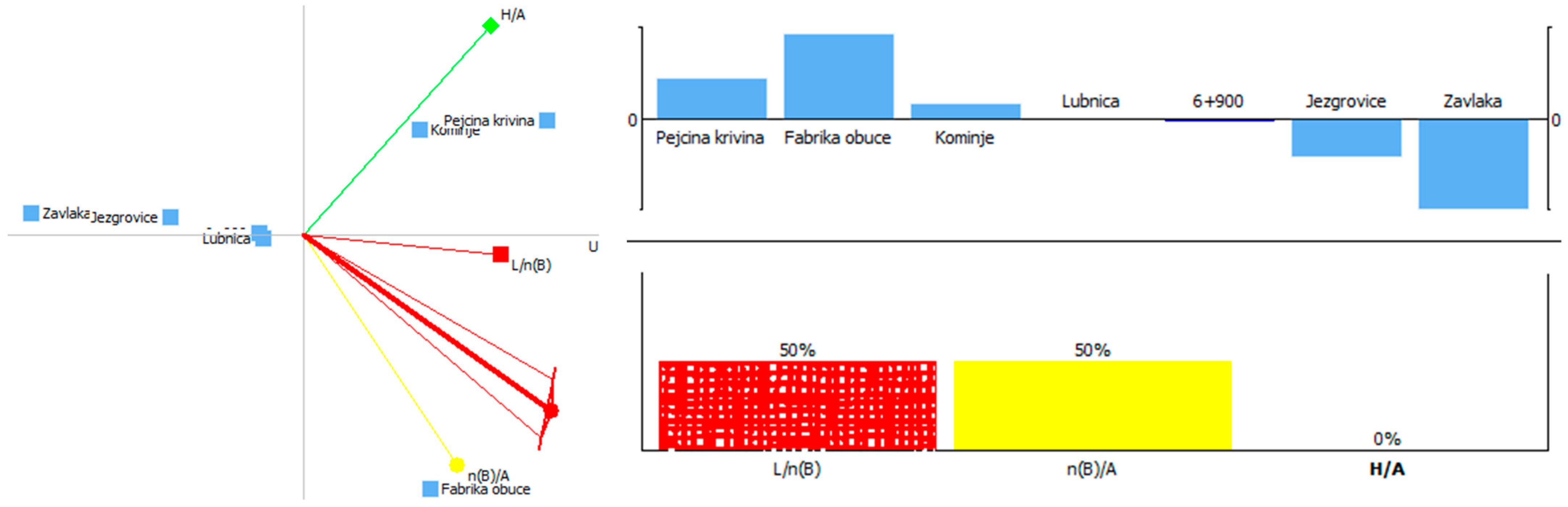
In the case of scenario
S7—combined scenario with equivalent weight coefficients was realized for the slopes “Pejčina krivina” with
Φ = 0.446 (
Figure 15).
For the scenario: S2 (maximization (for min. Preference) of the relationship between the length of the landslide (by road) and the number of wells L/n(B)) with Φ = 0.544, S4 (maximization of (for preference max) ratio of the number of wells and the surface of the landslide n(B)/A) with Φ = 0.545, S5 (maximization (for preference max) ratio of the quantity of drilling the surface of the landslide H/A) with Φ = 0.839 and S7 with an equivalent weight coefficients with Φ = 0.446 optimal solution is “Pajčina krivina”.
For scenarios: S3 (maximization (preference max) the ratio of the number of wells and surface of the landslide n(B)/A) with Φ = 0.859 and S6 (minimization (for preference max) the ratio of the amount of drilling over the surface of the landslide H/A) with Φ = 0.535 the optimal solution is “Footwear Factory”.
Based on the implemented optimization, it can be concluded that it forms a relationship:
the length of the landslide (by the way) and the number of wells L/n(B)—the minimum required number of wells is 3 (scenario S2),
number of wells and surface of landslide n(B)/A—the minimum required number of wells is 3 (scenario S3),
the amount of drilling on the surface of the landslide H/A—that the minimum required number of wells is 3 (scenario S5).
An identical solution was obtained for the combined scenario S7 with equivalent weight coefficients.
3.9. Sensitivity Analysis
Section 3.2 presents the results of optimization based on the given criteria
C1 (
L/
n(
B)),
C2 (
n(
B)
/A) and
C3 (
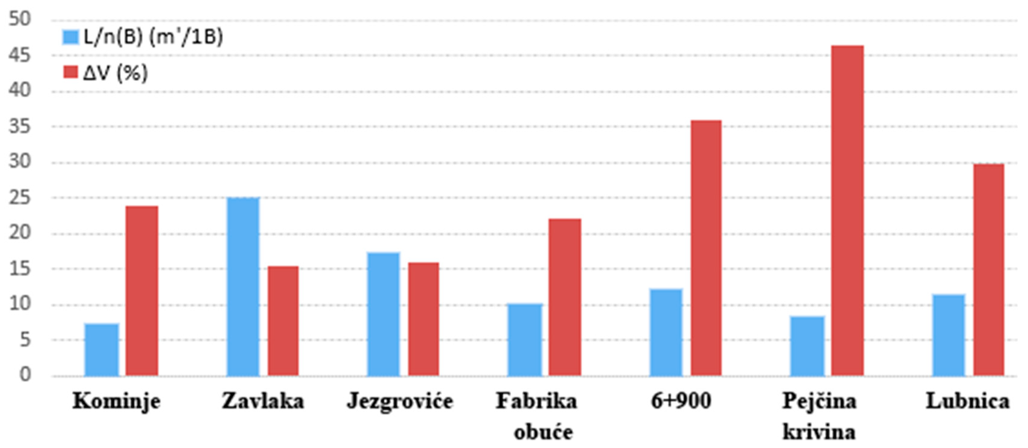
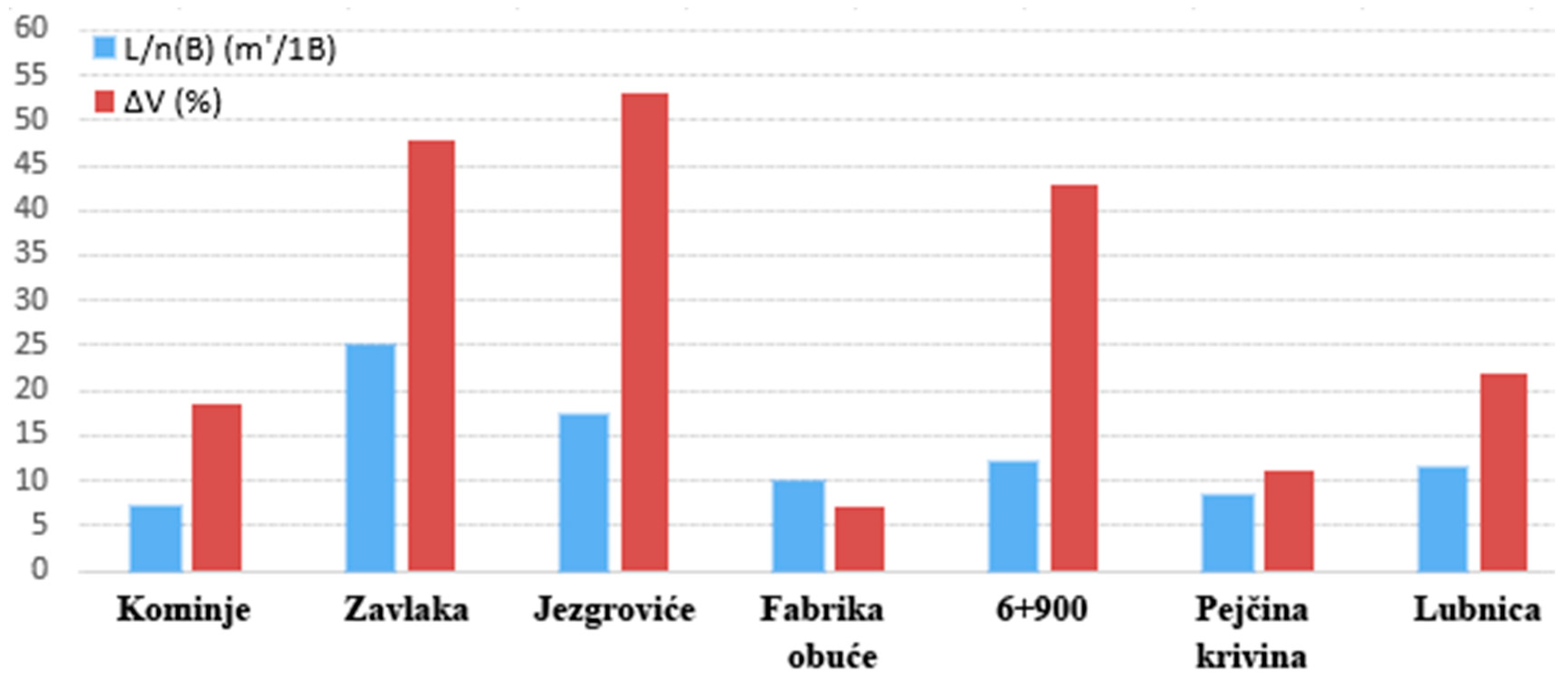
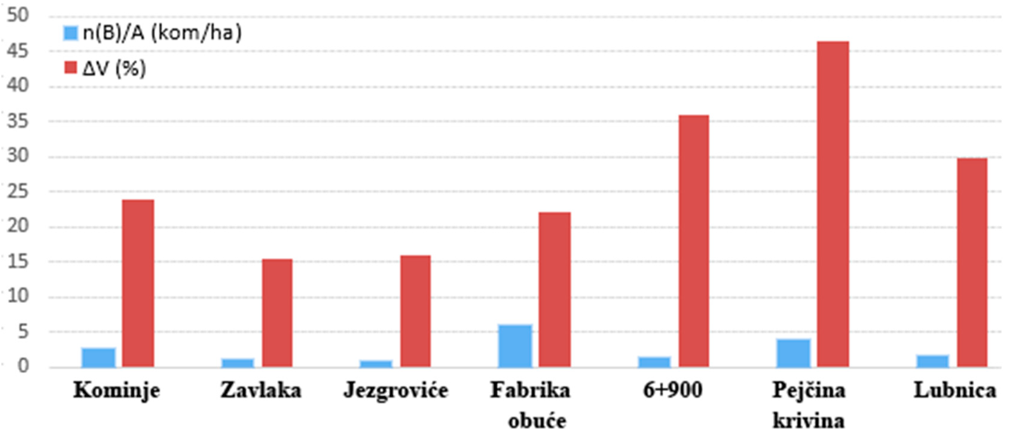
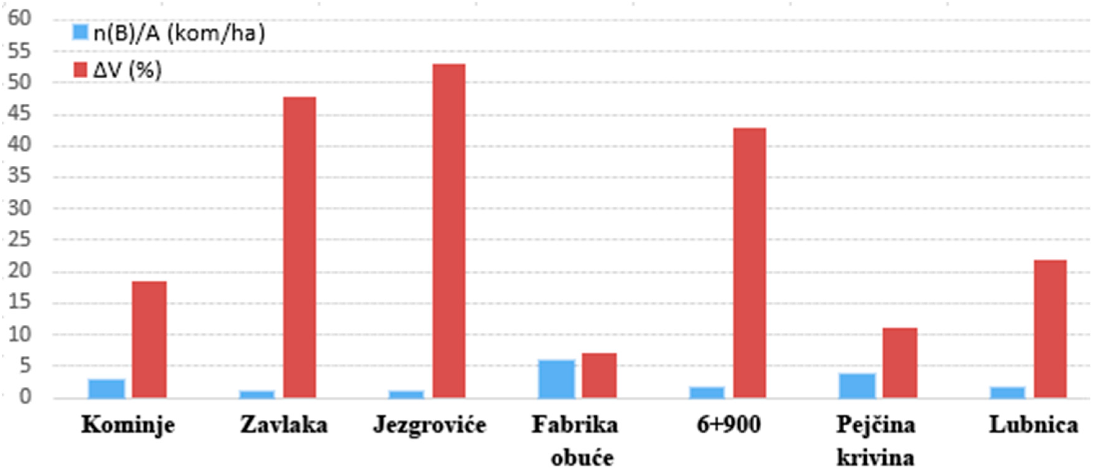
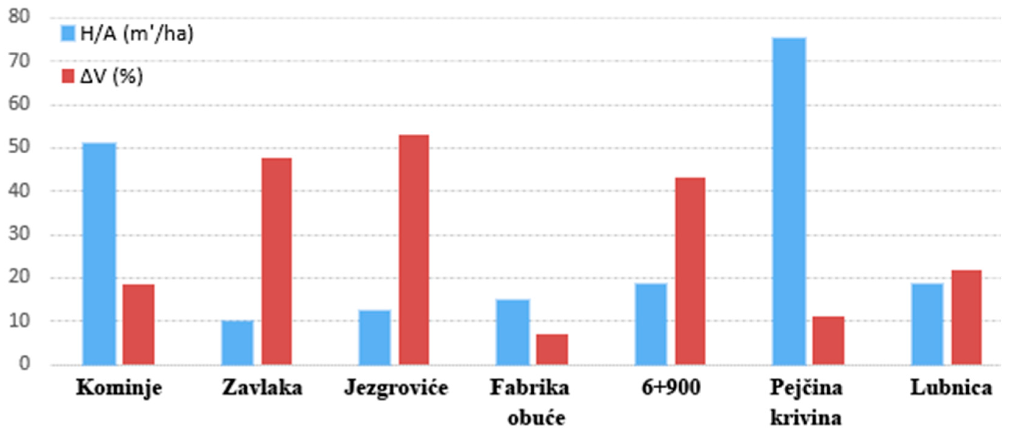
H/A). For the analysis of the sensitivity of the obtained results, in addition to these criteria, data on the increase in the amount of material ΔV of the performed state of landslide remediation Vi according to the amount of material of the project solution for landslide remediation were used.
Figure 16,
Figure 17,
Figure 18,
Figure 19,
Figure 20 and
Figure 21 shows the ratios of the increase in the amount of materials and works of the parameters of the third group (individual parameters) as a function of the considered remedied landslide. The units of measure are as follows: for the number of wells is
pcs (pieces), for the length of the landslide (along the road) m’, for the surface of the landslide ha (10,000 square meters = 10
4 m
2) and the amount of drilling m’.
Criterion C1 should have the lowest possible value, because, in that case, for the appropriate number of wells n(B), the engineering-geological profile of the terrain is better described. For criterion C1, and considering the parameter ΔV, a conditionally satisfactory solution for scenario S1 was obtained in the rehabilitation of the landslide “Zavlaka” and “Jezgrovići”, while a conditionally satisfactory solution for scenario S2 was obtained in the rehabilitation of the landslide “Footwear Factory”.
Criterion C2 should have the highest possible value, because, in that case, for the appropriate number of wells n(B), the engineering-geological profile of the terrain is better described. For criterion C2, and considering the parameter ΔV, no conditionally satisfactory solution was achieved for scenario S3 in landslide remediation, while conditionally satisfactory solution for scenario S4 was obtained in landslide remediation “Footwear Factory”.
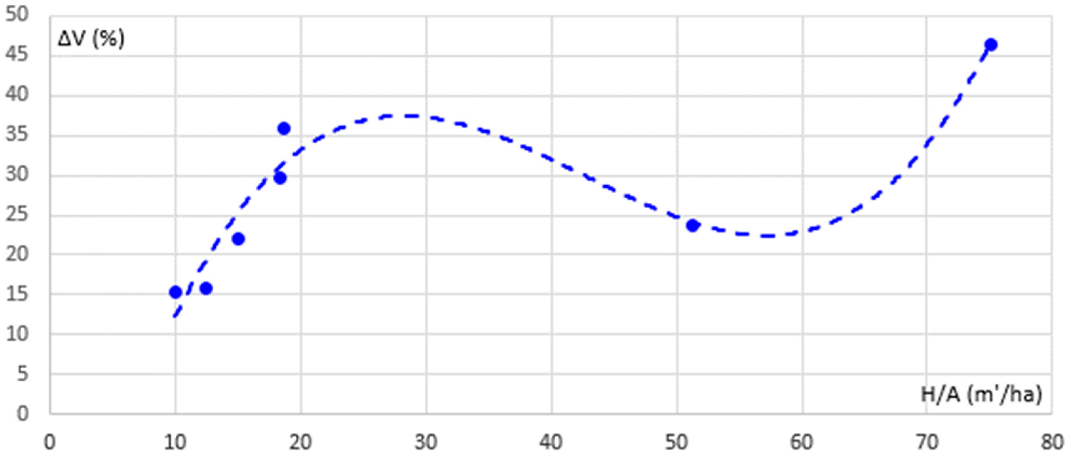
Criterion C3 should have the highest possible value, because, in that case, for the appropriate amount of drilling H, the engineering-geological profile of the terrain is better described.
With regards to this criterion, and considering the parameter ΔV, a conditionally satisfactory solution for scenario S5 was obtained in the rehabilitation of landslides “Zavlaka” and “Jezgrovići”, while a conditionally satisfactory solution for scenario S6 was obtained in the rehabilitation of landslide “Zavlaka”.
Additionally, the relations of previously presented parameters were considered and regression analysis was performed by searching for the optimal degree of polynomials for the selected function. Regression analysis (Reg), for the general case of the considered parameters, is represented by a polynomial function [
32]:
wherein
yReg considered the ordinate parameter according to regression analysis,
xReg considered the abscissa parameter according to regression analysis,
a1, …,
an unknown coefficients determined using the least squares method and matrix algebra. The general formula for least squares regression is:
where the other half of Expression (8) can be written as:
therefore, we obtain the following:
while in matrix form the previous expression reads:
By solving the matrix form (11) they are obtained:
where in:
Determination of unknown regression coefficients is carried out according to:
Since polynomials of higher degree are considered, the change in the value of the correlation coefficient is monitored:
wherein
xi and
yi are discrete values of abscissa and ordinate, respectively,
xm and
ym mean values.
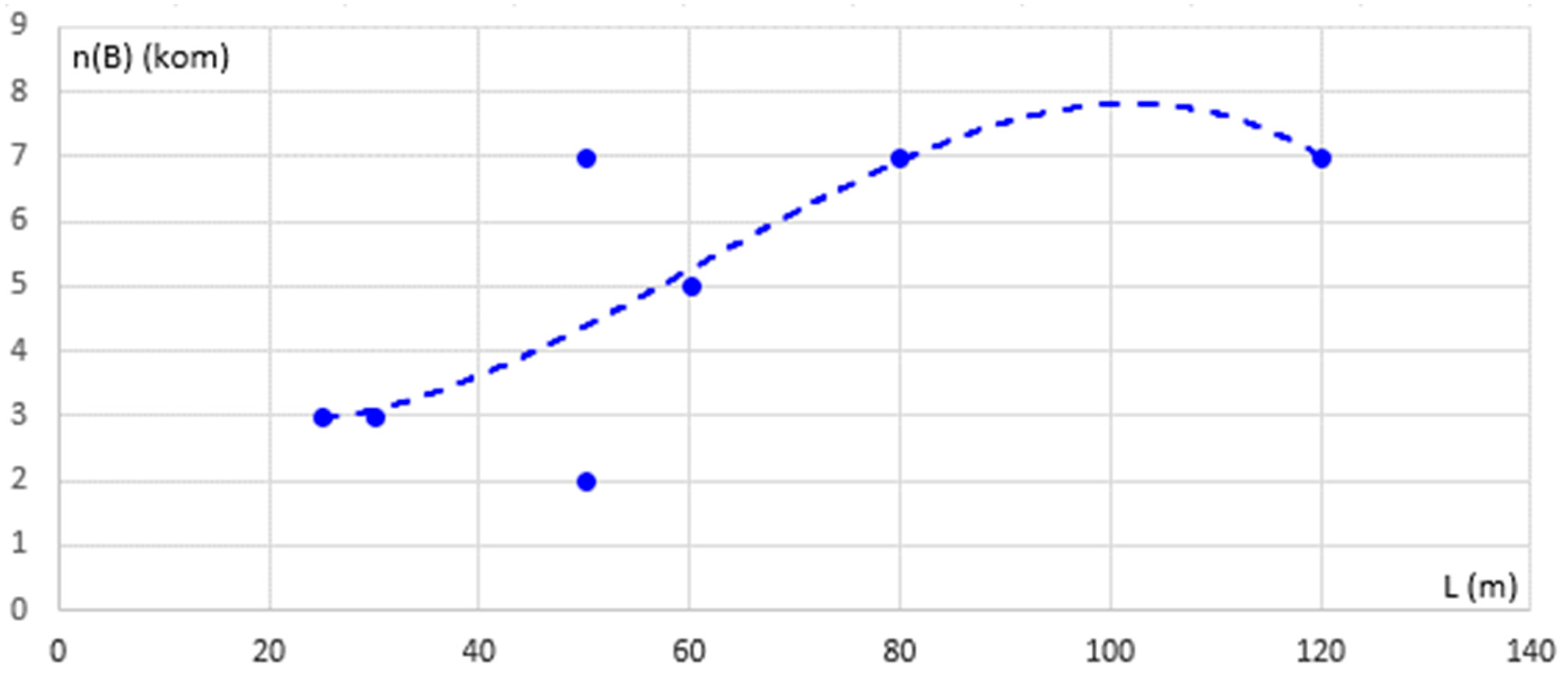
Both absolute and relative parameter values were considered in this group:
discrete values and regression analysis by polynomial function of landslide length (along the road) Li number of wells
n(
B) (
Figure 22):
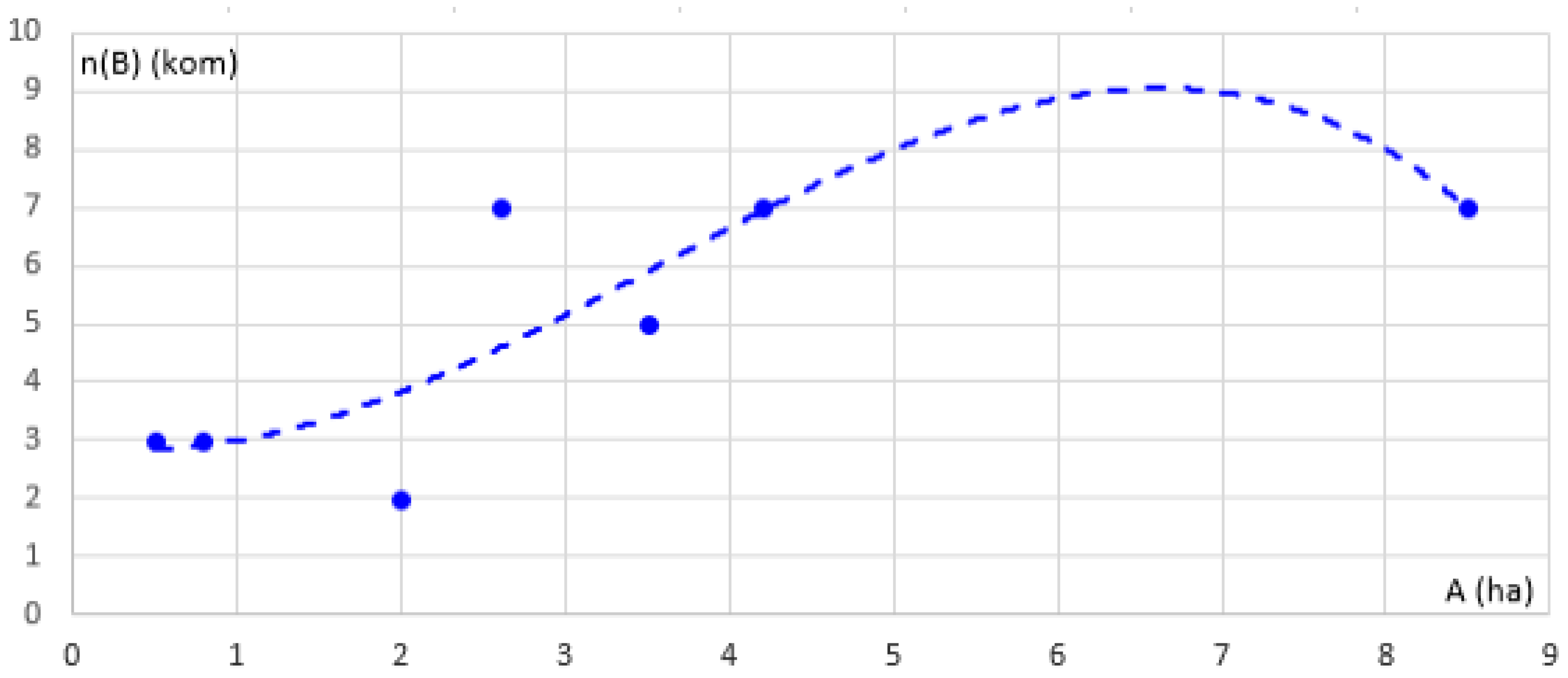
discrete values and regression analysis by polynomial function of landslide surface (along the road)
A and number of wells
n(
B) (
Figure 23):
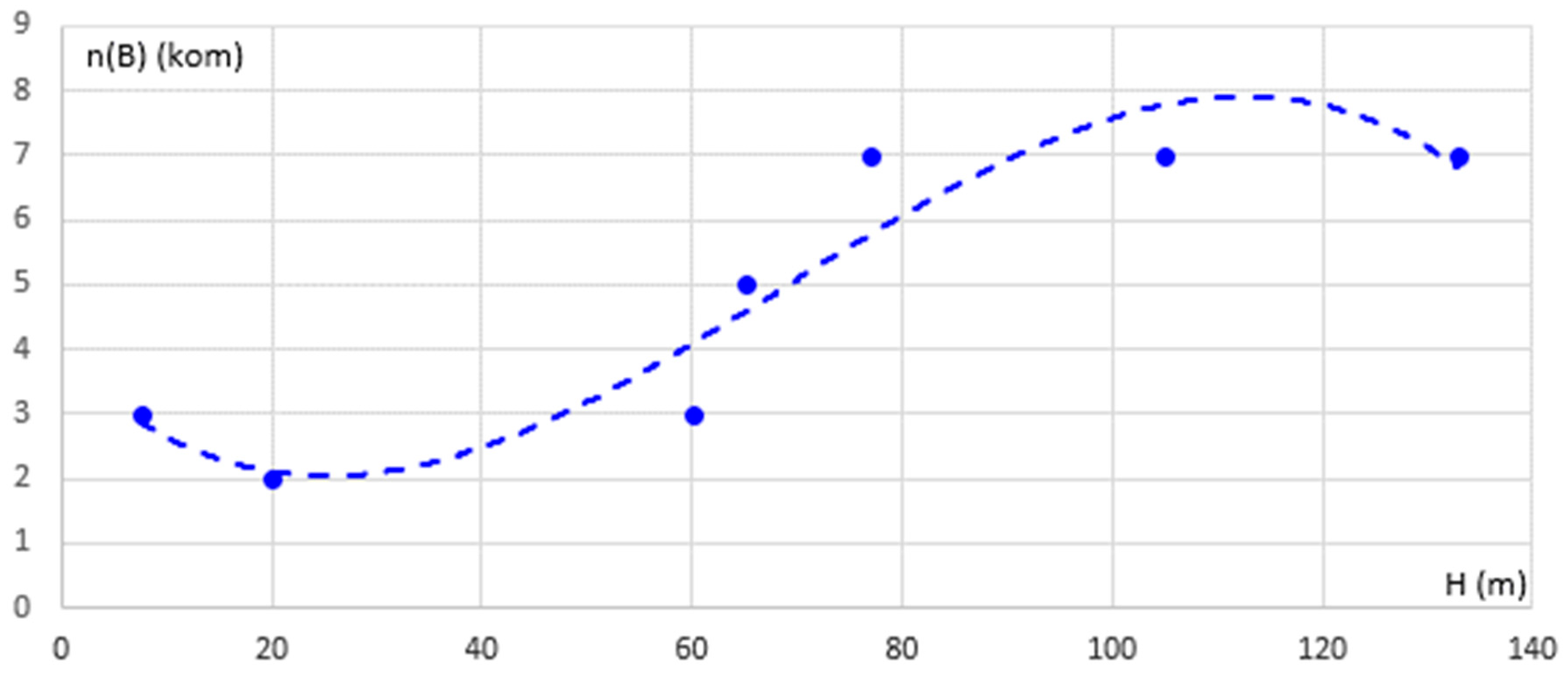
discrete values and regression analysis by polynomial function of the amount of drilling
H and the number of wells
n(
B) (
Figure 24):
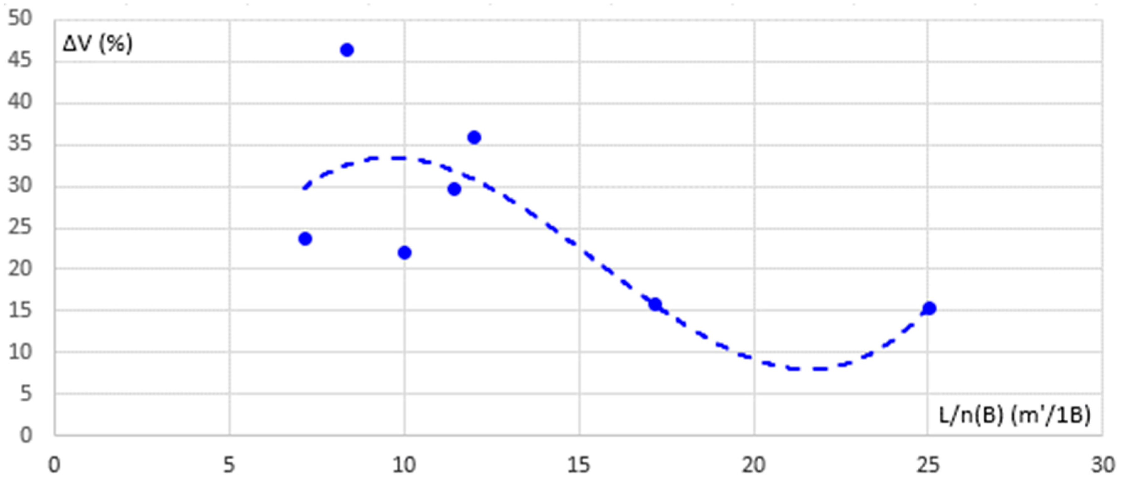
discrete values and regression analysis by polynomial function of the ratio of the length of the landslide (along the road) Li of the number of wells
n(
B) and the ratio of the increase in the amount of excavation (performed/projected excavation)) ΔV (
Figure 25):
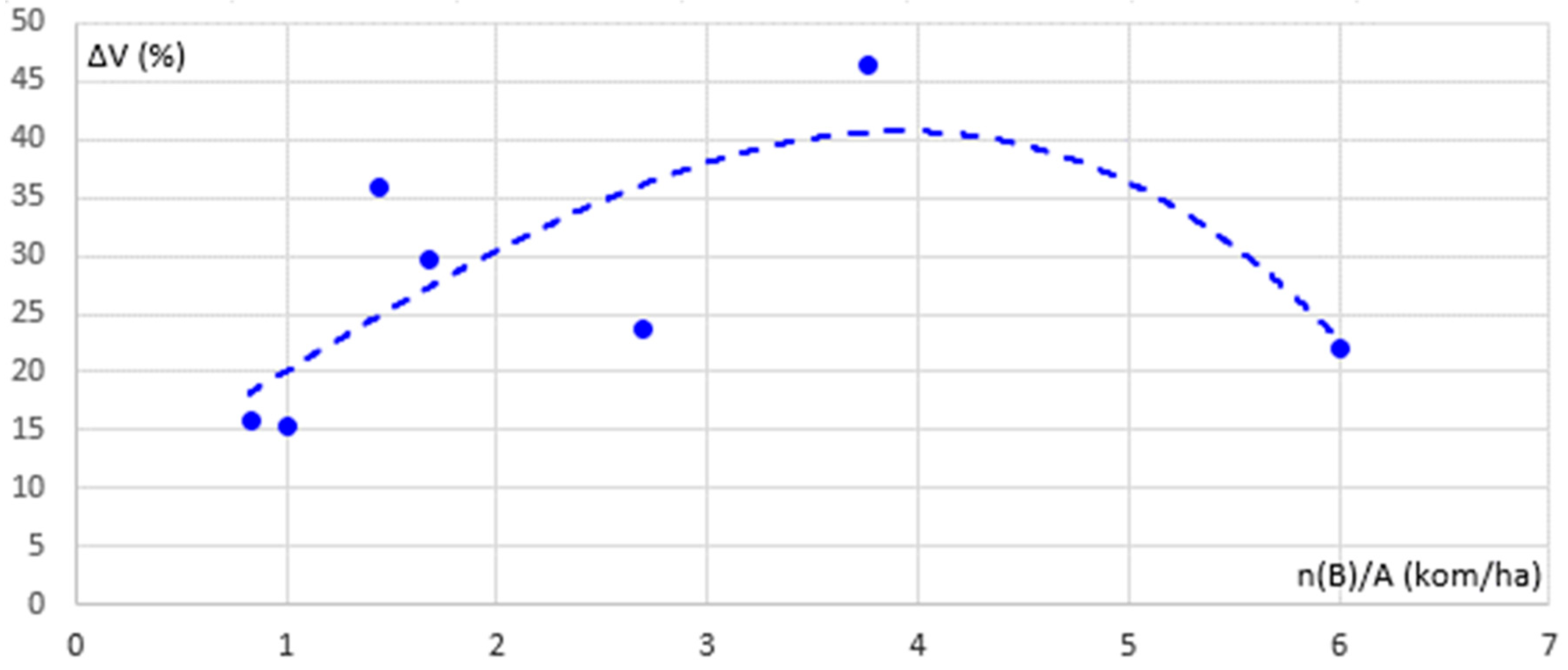
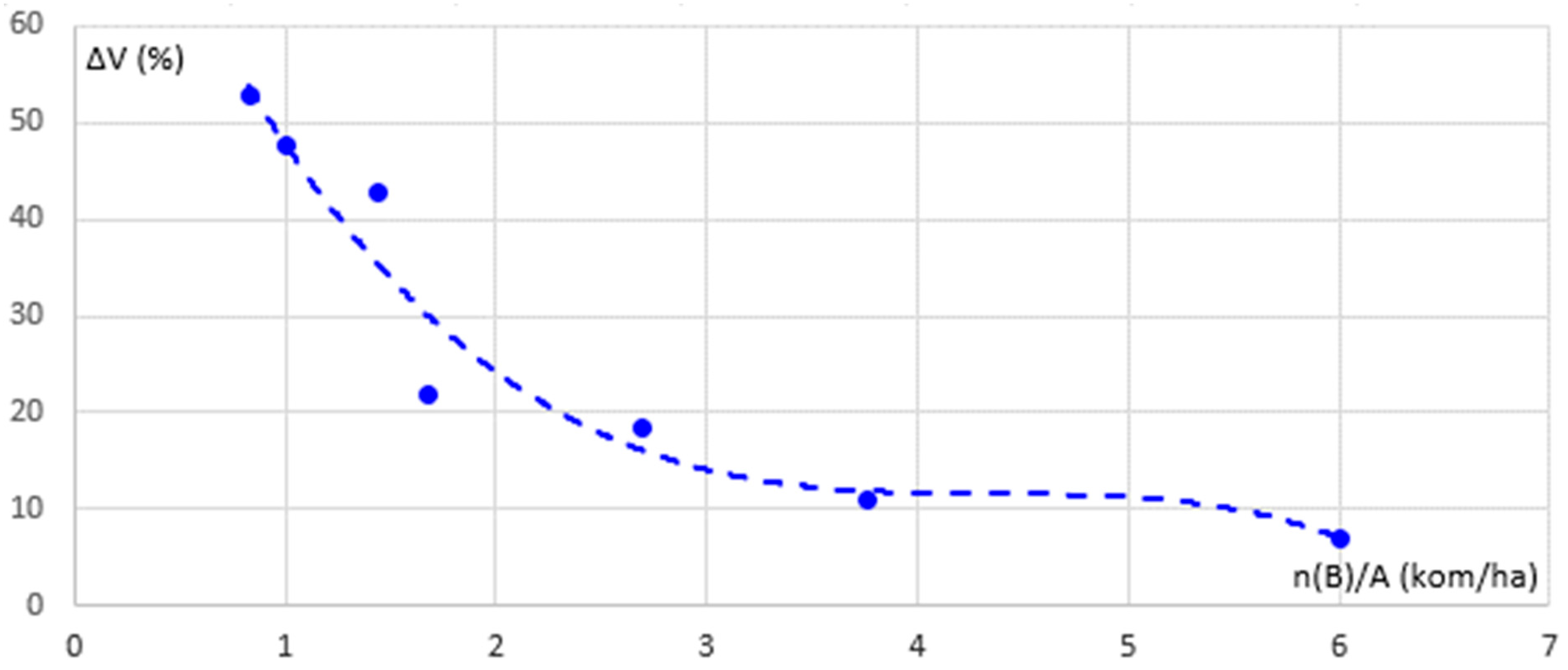
discrete values and regression analysis by polynomial function of the ratio of the number of wells
n(
B) and the landslide area
A and the ratio of the increase in the amount of excavation (performed/projected excavation) ΔV (
Figure 26):
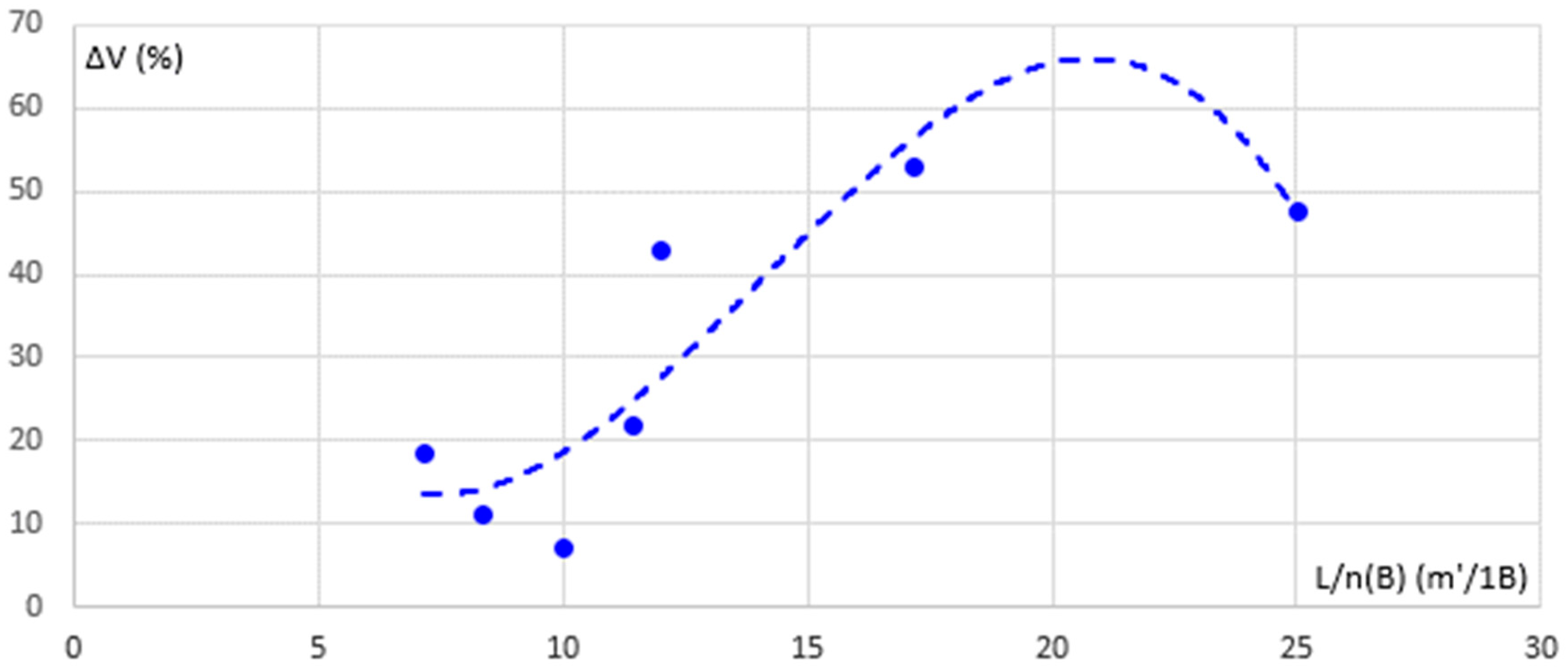
discrete values and regression analysis by polynomial function of the relationship between the length of the landslide (along the road)
L and the number of wells
n(
B) and the relationship between the increase in the amount of embankment (constructed/designed embankment)) ΔV (
Figure 27):
discrete values and regression analysis by polynomial function of the ratio of the number of wells
n(
B) and the landslide surface
A and the ratio of the increase in the amount of embankment (constructed/designed embankment)) ΔV (
Figure 28):
discrete values and regression analysis by polynomial function of the ratio of the amount of drilling
H and the surface of landslide
A and the ratio of increasing the amount of excavation (performed/projected excavation) ΔV (
Figure 29):
discrete values and regression analysis by polynomial function of the ratio of the amount of drilling
H and the surface of landslide
A and the ratio of increasing the amount of embankment (constructed/designed embankment) ΔV (
Figure 30):
Figure 22 shows the discrete values and regression analyzes by polynomial function of the third group (absolute and relative values) of parameters:
Derived expressions ((19)–(24)), from regression analyses by polynomial function can be used for practical purposes for analyzes of remediation of other landslides, taking into account the extreme values of the number of wells n(B) from this research.
4. Conclusions
The research conducted in this paper refers to the issue of multi-criteria optimization solutions for the repair of landslides. By optimizing the function of the number of wells in additional soil erosion through several scenarios, for selected preferences, solutions were obtained according to predefined scenarios and based on the ranking of the flow function. The research showed that it is from the ratio of the length of the landslide (along the road) and the number of wells L/n(B), the ratio of the number of wells and surface of the landslide n(B)/A and the ratio of the amount of drilling over the surface of the landslide H/A that the minimum required number of boreholes is 3. An identical solution was obtained for the combined scenario with equivalent weight coefficients. However, by expanding the population of the number of landslides using statistical distribution and stochastic modeling, and by considering the theory of probability, it was shown that the required number of boreholes a n(B) is significantly higher than 3.
As one of the most important examples of what should be done in order to improve the research, it is more accurate to determine the weight of certain criteria and a potential addition to the existing list of criteria, with the recommendation to use the so-called Delphi method. The Delphi method is based on collecting, analyzing, and harmonizing the answers from a large number of experts to certain questions in the field under research. By hiring a certain number of experts who provide answers to precisely designed and formulated questions through an anonymous survey, and which can usually have from 10 to 12 questions (in some cases much higher), we would obtain more precisely determined weights of certain criteria. The Delphi method could be implemented in two or three rounds. In the first round of the survey, experts would provide answers to the questions asked in the questionnaire. The obtained answers would then be analyzed and systematized, and based on them, another questionnaire is made. In the second round, the experts were informed about the results of the first round of the survey, through certain statistical indicators, and would again answer the questions asked. Sometimes the third round is conducted according to the procedure described for the second round of the survey.


 ,
, 


