Modification of the Logarithm Methodology of Additive Weights (LMAW) by a Triangular Fuzzy Number and Its Application in Multi-Criteria Decision Making

Abstract

The Logarithm Methodology of Additive Weights (LMAW) method is a very young method and in its basic form is defined for crisp values. In this paper, the LMAW method was improved by being modified with triangular fuzzy numbers. The modification significantly improved the capacity of the LMAW method to consider uncertainty in decision making. The special importance of the method is reflected in a relatively simple mathematical apparatus due to which it is possible to define, with high quality, weight coefficients of criteria and rank alternative solutions in uncertain environments. The method was tested in solving the problem of the location selection for a landing operations point (LOP) in combat operations of the army. The validation of the obtained results was performed: (1) by means of comparison with the Fuzzy Simple Additive Weighting (FSAW) Method, the Fuzzy Multi-Attributive Border Approximation area Comparison (FMABAC), the fuzzy Višekriterijumsko KOmpromisno Rangiranje (FVIKOR), the fuzzy COmpressed PRoportional ASsessment (FCOPRAS), and the fuzzy Multi Attributive Ideal-Real Comparative Analysis (FMAIRCA); (2) by means of sensitivity analysis by changing the weight coefficients of criteria; and (3) using simulation software. In comparison with other methods, the quality of the ranking of alternative solutions was confirmed, which highlighted the special importance of the fuzzy LMAW method relative to that of certain standard methods, respectively, the ones that are often used and confirmed in practice. On the other hand, the sensitivity analysis, including the changing of the weight coefficients of criteria, showed that the model could tolerate smaller errors in defining the weight coefficients of criteria, and it provided stable results. Finally, the validation of results achieved with the use of simulation software confirmed the obtained output results. The output results confirmed the quality of the modified method.

1. Introduction

Decision making is an important aspect of human life. It is present in everyday human activities, from making daily and individual decisions, to decisions that are important to a group of people or even to the wider community. The importance of decision making has conditioned the development of a large number of techniques—methods that support the decision-making process, such as by helping decision makers to perceive a problem more comprehensively and make a rational decision. Increasingly, the new methods of multicriteria decision making have appeared in contemporary literature. Some of them are widely used, while others remain almost unknown. Some methods are developed for the complete process, for defining weights of criteria and ranking alternatives, and when using some of them, weights of criteria can be defined or the alternatives can be ranked. The following methods can be singled out as frequently used: Simple Additive Weighting (SAW) [1], ELimination Et Choice Translating REality I (ELECTRE I) [2], ELECTRE II [3], ELECTRE III [4], ELECTRE IV [5], DEcision-MAking Trial and Evaluation Laboratory (DEMATEL) [6], Analytic Hierarchy Process (AHP) [7], Technique for Order of Preference by Similarity to Ideal Solution (TOPSIS) [8], Preference Ranking Organization METHod for Enrichment of Evaluations I (PROMETHEE I) [9], PROMETHEE II [10], TOmada de Decisao Interativa Multicriterio (TODIM) [11], CRiteria Importance Through Intercriteria Correlation (CRITIC) [12], COmpressed PRoportional ASsessment (COPRAS) [13], Measuring Attractiveness through a Categorical-Based Evaluation TecHnique MACBETH [14], Višekriterijumsko KOmpromisno Rangiranje (VIKOR) [15], PROMETHEE III [16], Data Envelopment Analysis (DEA) [17], Step-wise Weight Assessment Ratio Analysis (SWARA) [18], Best-Worst Method (BWM) [19], Characteristic Objects METhod COMET [20], COmbinative Distance-based ASsessment (CODAS) [21], etc.

One method from the set of newer methods is the Logarithm Methodology of Additive Weights—LMAW [22]. This method was developed in order to define weight coefficients and rank alternatives. So far, the LMAW method has been applied in a number of papers only to define weight coefficients of criteria, both in its basic and modified form [23,24,25]. In this paper, the LMAW method was modified using fuzzy numbers (FLMAW) and was used both for the calculation of weight coefficients of criteria and for the evaluation of alternative solutions.

2. Theoretical Background

The application of the FLMAW method in this paper is presented with the example of selecting a location for river crossing to illustrate an instance of decision-making in the army. The MCDM has taken a significant place in decision-making in the army, and it is especially important in decision-making in combat operations. When there is a river, lake or some other water obstacle in the zone of a combat operation, which needs to be crossed, specialized means are used for that purpose. A water barrier, which in most cases is a river, is crossed, including the application of specific procedures for that purpose, depending on whether or not the enemy is acting at the location where the river is crossed or forced crossed [26]. One of the hardest battle operations is forced river crossing, a situation when a river is crossed at the same time as enemy actions are applied on the units performing the river crossing. That is the reason why the procedure of river crossing is divided into three phases [26]. In the first phase, the river is conquered by using fast means (usually different types of boats and amphibious transporters), with the goal of conquering a part of the opposite bank and minimizing the action of the enemy. In the second phase, transport is organized with different types of scaffolding, when, in addition to humans, larger caliber weapons are also transported. In some situations, depending on the needs of the operation, bridges (usually made of pontoon material) are established, over which almost all means of war equipment can be transported to the opposite bank.

This paper deals with the selection of the location for river crossing in the most critical, first phase, namely the selection of the location of a landing operation point (LOP) over the water barrier in the Serbian Army using MCDM as a support for decision making. In this phase, there is a large number of uncertain, mutually contradictory factors that make the process of decision making at the location of the landing operation point more complex. Therefore, the application of the MCDM methods is indispensable in solving this problem.

The solving of military problems using the application of MCDM methods is becoming more and more present in the public literature. Jokić et al. [27] published research on the selection of the fire position of mortar units using the LBWA-Fuzzy MABAC model. Božanić et al. [28] used the neuro-fuzzy model for the selection of the course of action in defense operations. Radovanović et al. [29] made the selection of the most efficient procedure for rectification of the optical sight of the long-range rifle by applying the model of fuzzy AHP-VIKOR. By using the Decision expert (DEX) method, Jokić et al. [30] showed the selection of Rifle Caliber in the Rearming Process. Radovanović et al. [31] analysed the correctness and precision of the automatic rifle shooting by applying the AHP method. In the paper by Radovanović et al. [32] the analysis of anti-armor missile systems using the hybrid AHP-VIKOR method was presented. Goztepe et al. [33] used a multicriteria interval-valued intuitionistic fuzzy decision-making method for the location selection analysis approach for the maintenance facility for military armored vehicles. Goztepe [34] applied the ANFIS model for the selection of the best fire support plan on the battlefield. The ANFIS model is presented also during the selection of the construction machines for the needs of the engineering units of the Serbian Army [35]. Devetak and Terzić [36] (2011) used the AHP method in selecting an optimal tactic radio communication system. Deveci et al. [37] investigated various types of fuzzy sets that can be used in military problems under uncertainty. Sánchez-Lozano and Rodríguez [38] use the Fuzzy Reference Ideal Method (FRIM) for the selection of the best military advanced training aircraft in the Spanish Air Force. Sánchez-Lozano et al. [39] showed a combination of the MCDM methodology (the AHP and TOPSIS methods) with the geographic information systems (GIS) used to carry out prioritization of obsolete military coastal batteries with the aim of transforming them into touristic, scientific, and cultural places of interest. De Almeda et al. [40] used the Simple Aggregation of Preferences Expressed by Ordinal method Vectors—Multi Decision Makers (SAPEVO-M) and VIKOR methods to select the most suitable city as the headquarters of the Second Fleet of the Brazilian Navy. In the paper, Moreira et al. [41] showed the ranking of the attack helicopters of the Brazilian Navy using the PROMETHEE and SAPEVO-M1 methods. Problems related to river crossing are not discussed considerably. In the paper by Božanić and Pamučar [42], the selection of the locations for placing the pontoon bridge by applying the fuzzy logic system was discussed. Božanić et al. [43] used the fuzzy logic system for the risk assessment in river crossing. The selection of the location of the LOP is presented as an example in the paper by Pamučar et al. [44] in which interval-valued fuzzy-rough numbers and the MAIRCA method were used.

According to everything presented, this paper provides two basic novelties. The first is methodological because the fuzzification of a relatively new method is presented and the results obtained by the fuzzified method are evaluated. Another novelty is related to solving the case study of the LOP selection, where at the end of the research the results are confirmed by the use of a simulation software, which confirms the quality of the FLMAW method.

The next part of the paper is organized into three parts. The third part describes the FLMAW method. In the fourth part, the criteria on which the selection of the LOP location depends are presented and the FLMAW method is applied in specific examples and with a detailed calculation presented. In the fifth part, the validation of the obtained results is performed through three procedures: comparison of the obtained results with other MCDM methods, sensitivity analysis through changing the weight coefficients of the criteria and checking the results in the simulation software.

3. Description of the Methodology Applied

3.1. Model Description

The model described in this paper has the purpose of solving the LOP location issue. Solving such an issue is specific due to significant uncertainty. The first set of uncertain elements appears during the defining of the criteria for the LOP selection. In defining the weight coefficients of the criteria, a new set of uncertain elements appears. Finally, a similar situation occurs in the process of ranking alternatives. Therefore, in this model the problems are solved by using group (expert) decision making. Additionally, in order to reduce uncertainty in the process of decision making, fuzzy numbers and the LMAW method are used. In addition to solving a specific problem, the aim of the paper is to present in detail the FLMAW methods, in order to test this method with other issues.

The model of the LOP location selection is provided in Figure 1.

As can be seen from Figure 1, the model has two phases: the phase of application of the FLMAW method (definition of weight coefficients of criteria and ranking of alternatives), and the phase of validation of the obtained results. The applied methods are presented below.

3.2. Fuzzy Number

Fuzzy logic is an area that has developed significantly in recent years. The basic settings of fuzzy logic are set by Lotfi Zadeh [45,46,47], and those were enough to provide further development of the area of fuzzy logic causing its wider application in the practice.

In conventional sets, the membership of one element to a set is unambiguously defined, a certain element can or cannot belong to a set. In fuzzy sets, the membership of one element to a particular set is not precisely defined; the element can more or less form part of a set, which makes fuzzy logic closer to human perception compared with conventional logic. Such a feature allows fuzzy logic to quantify information that is considered imprecise in classic logic. The existence of seemingly inaccurate information, which is well processed by fuzzy logic, is a very common occurrence in the social sciences, and thus in decision-making processes.

The quantification of uncertainty has advanced significantly in modern science. Today, in addition to classic fuzzy numbers, a variety of other fuzzy approaches are used, such as: type-2 fuzzy numbers, intuitionistic fuzzy numbers, Pythagorean fuzzy numbers, etc. In addition, other approaches are used to quantify uncertainty, such as: rough numbers, gray numbers, D numbers, etc. In this paper, the fuzzification of the applied method was carried out with classic triangular fuzzy numbers. Checking the obtained results, it was found that classic triangular fuzzy numbers described quite well the uncertainty arising when solving the decision-making problems presented in this paper. Accordingly, the following part of the paper presents the most basic elements that are sufficient to understand the application of triangular fuzzy numbers.

Fuzzy set A is defined as a set of ordered pairs:

$$A=\left\{\left(x,{\mu }_A\left(x\right)\right)\left|x\in X,0\le {\mu }_A\left(x\right)\le 1\right.\right\},$$

(1)

where:

-

X—universal set or a set of considerations based on which is defined the fuzzy set A;

-

μA(x) membership function of the element x (x ∈ X) to the set A; membership function can have any value between 0 and 1, and as the value of the function is closer to one, the membership of the element x to the set A is higher, and vice versa.

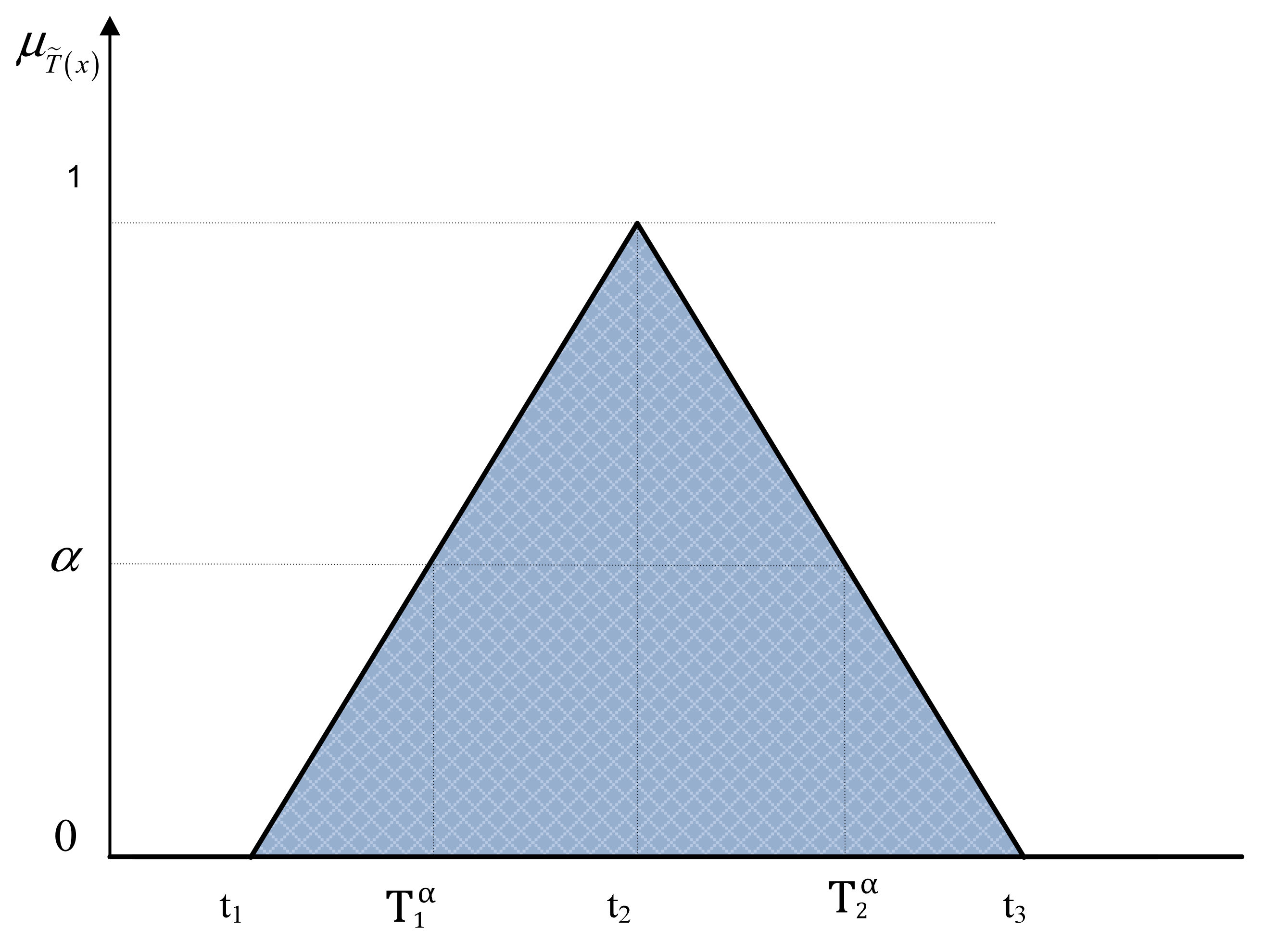
Triangular fuzzy number T = (t₁, t₂, t₃) is presented in Figure 2, where t₁ presents the left, and t₃ the right distribution of the confidence interval of the fuzzy number T and t₂, the point in which the membership function of the fuzzy number has its maximum value.

The concept based on which the fuzzy number is expressed using confidence intervals and relevant confidence degrees is suggested by Kaufmann and Gupta [48]. Considering Figure 2, the confidence interval presents a closed set [t₁, t₃]. Therefore, a fuzzy variable can have the values only from the confidence interval. Defining confidence interval of every fuzzy variable is the task of the planner, and the most natural and often used solution is to adopt a confidence interval so that it matches the physical limits of the variable [49]. If the variable has no physical origin, some of the standard ones are adopted or it is defined as an abstract confidence interval [42]. The degree of membership is the value related to the confidence interval. In Figure 2, the confidence interval with the membership degree α can be observed, marked as $\left[T_1^{\alpha },T_2^{\alpha }\right]$.

3.3. Fuzzy Logarithm Methodology of Additive Weights

In order to define the weight coefficients of the criteria and select the best alternative, modified Logarithm Methodology of Additive Weights (LMAW) is used. This method in its basic form (crisp version) was presented for the first time in the paper by Pamučar et al. [22]. In this paper, the modification (fuzzification) of the LMAW method is performed by applying triangular fuzzy numbers.

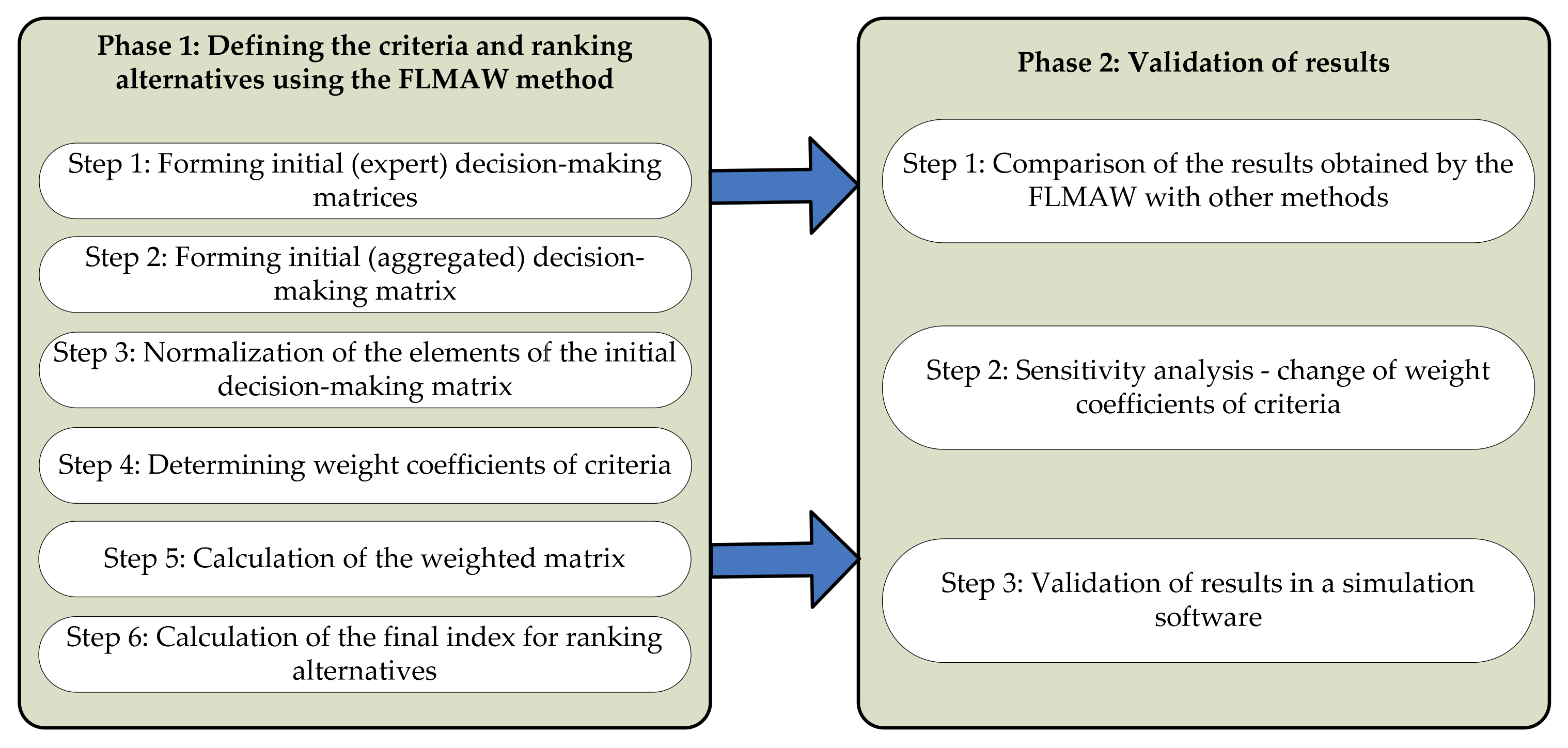
Further in the paper the steps of the fuzzy LMAW (FLMAW) are presented. The FLMAW method consists of six steps:

Step 1: Forming initial (expert) decision-making matrices (${\tilde{X}}^e$). In the first step, every expert ($e$) from the group of $k$ experts ($1\le e\le k$) defines one initial decision-making matrix, in which he performs the evaluation of $m$ alternatives $A=\left\{A_1,A_2,\dots ,\hspace{0.17em}{A}_m\right\}$ in relation to $n$ criteria $C=\left\{C_1,\hspace{0.17em}{C}_2,\dots ,\hspace{0.17em}{C}_n\right\}.$ Accordingly, for every expert the matrix ${\tilde{X}}^e={\left[{\tilde{\vartheta }}_{ij}^e\right]}_{m\times n}$ is obtained, where ${\tilde{\vartheta }}_{ij}^e$ presents fuzzy value based on which the expert $e$ evaluated $i$-th alternative by $j$-th criterion. The evaluation is made based on quantitative indicators or based on fuzzy linguistic descriptors, depending on the type of criterion.

Step 2: Forming initial (aggregated) decision-making matrix ($\tilde{X}$). Aggregation of initial (expert) matrices into one aggregate matrix is made by applying the Bonferroni aggregator, according to the Equation (2):

$$\begin{array}{l}{\tilde{\vartheta }}_{ij}=\left(\frac{1}{k(k-1)}{\displaystyle \sum _{\begin{array}{l}i,j=1\\ i\ne j\end{array}}^k{\tilde{\vartheta }}_i^{(e)p}{\tilde{\vartheta }}_j^{(e)q}}\right)=\\ \left\{{\left(\frac{1}{k(k-1)}{\displaystyle \sum _{\begin{array}{l}i,j=1\\ i\ne j\end{array}}^k{\vartheta }_i^{(l_e)p}{\vartheta }_j^{(l_e)q}}\right)}^{\frac{1}{p+q}},{\left(\frac{1}{k(k-1)}{\displaystyle \sum _{\begin{array}{l}i,j=1\\ i\ne j\end{array}}^k{\vartheta }_i^{(m_e)p}{\vartheta }_j^{(m_e)q}}\right)}^{\frac{1}{p+q}},{\left(\frac{1}{k(k-1)}{\displaystyle \sum _{\begin{array}{l}i,j=1\\ i\ne j\end{array}}^k{\vartheta }_i^{(r_e)p}{\vartheta }_j^{(r_e)q}}\right)}^{\frac{1}{p+q}}\right\}\end{array}$$

(2)

where ${\tilde{\vartheta }}_{ij}$ presents averaged values obtained by applying the Bonferroni aggregator; $p,q \ge 0$ present stabilization parameters of the Bonferroni aggregator, e presents the e-th expert $1\le e\le k$, l—the left distribution of a fuzzy number, r—the right distribution of a fuzzy number, and m—the value in which the membership function of a fuzzy number is equal to one. Before the aggregation, the quantification of linguistic criteria is performed.

Step 3: Normalization of the elements of the initial decision-making matrix. Applying the Equation (3), the normalized matrix $\tilde{\Upsilon }={\left[{\tilde{\vartheta }}_{ij}^{\prime }\right]}_{m\times n}$ is obtained:

$${{\tilde{\vartheta }}^{\prime }}_{ij}^{}=\left\{\begin{array}{l}1+\frac{{\tilde{\vartheta }}_{ij}^{}}{{\tilde{\vartheta }}_j^{(+)}}=\left(1+\frac{{\vartheta }_{ij}^{(l)}}{{\vartheta }_j^{(+)}},1+\frac{{\vartheta }_{ij}^{(m)}}{{\vartheta }_j^{(+)}},1+\frac{{\vartheta }_{ij}^{(r)}}{{\vartheta }_j^{(+)}}\right) if j\in B,\\ 1+\frac{{\tilde{\vartheta }}_j^{-}}{{\tilde{\vartheta }}_{ij}^{}}=\left(1+\frac{{\vartheta }_j^{-}}{{\vartheta }_{ij}^{(r)}},1+\frac{{\vartheta }_j^{-}}{{\vartheta }_{ij}^{(m)}},1+\frac{{\vartheta }_j^{-}}{{\vartheta }_{ij}^{(l)}}\right)if j\in C.\end{array}\right.$$

(3)

where ${{\tilde{\vartheta }}^{\prime }}_{ij}^{}$ presents normalized values of the initial decision-making matrix, while ${\vartheta }_j^{+}=\max ({\tilde{\vartheta }}_j^{(r)})$, and ${\vartheta }_j^{-}=\min ({\vartheta }_j^{(l)})$, and l presents the left distribution of a fuzzy number, r the right distribution of a fuzzy number, and m the value where the membership function of a fuzzy number is equal to one.

Step 4: Determining weight coefficients of criteria. In order to determine weight coefficients of the criteria, certain experts are supposed to be engaged $E=\left\{E_1,E_2,\dots ,E_k\right\}$.

Step 4.1: Prioritization of criteria. Based on the values from the predefined fuzzy linguistic scale the experts prioritize the criteria $C=\left\{C_1,\hspace{0.17em}{C}_2,\dots ,\hspace{0.17em}{C}_n\right\}$. To the criterion with higher significance is assigned the higher value from the fuzzy linguistic scale, and vice versa. This way the priority vectors ${\tilde{P}}^e=\left({\tilde{\gamma }}_{C1}^e,{\tilde{\gamma }}_{C2}^e,\dots ,{\tilde{\gamma }}_{Cn}^e\right)$ are defined, for every expert separately, where ${\tilde{\gamma }}_{Cn}^e$ presents the value from the fuzzy linguistic scale which the expert e ($1\le e\le k$) assigned to the criterion n.

Step 4.2: Defining the absolute fuzzy anti-ideal point (${\tilde{\gamma }}_{AIP}$). This value is defined by a decision maker, and it presents a fuzzy number which is smaller than the smallest value from the set of all priority vectors.

Step 4.3: Defining fuzzy relation vector (${\tilde{R}}^e$). Applying the Equation (4), the relation between the elements of the priority vector and the absolute anti-ideal point (${\gamma }_{AIP}$) is determined.

$${\tilde{\eta }}_{Cn}^e=\left(\frac{{\tilde{\gamma }}_{Cn}^e}{{\tilde{\gamma }}_{AIP}^{}}\right)=\left(\frac{{\gamma }_{Cn}^{(l)e}}{{\gamma }_{AIP}^{(r)}},\frac{{\gamma }_{Cn}^{(m)e}}{{\gamma }_{AIP}^{(m)}},\frac{{\gamma }_{Cn}^{(r)e}}{{\gamma }_{AIP}^{(l)}}\right)$$

(4)

Applying the Equation (4), the relations vector of the expert e ($1\le e\le k$): $R^e=\left({\tilde{\eta }}_{C1}^e,{\tilde{\eta }}_{C2}^e,\dots ,{\tilde{\eta }}_{Cn}^e\right)$ is obtained.

Step 4.4: Determining vectors of weight coefficients $w_j^e={\left({\tilde{w}}_{}^e{}_1,{\tilde{w}}_{}^e{}_2,\dots ,{\tilde{w}}_{}^e{}_n\right)}^T$, for every expert separately. Fuzzy values of the weight coefficients of criteria for the expert e ($1\le e\le k$) are obtained by applying the Equation (5):

$${\tilde{w}}_j^e=\left(\frac{\ln \left({\tilde{\eta }}_{Cn}^e\right)}{\ln \left({\displaystyle \prod _{j=1}^n{\tilde{\eta }}_{Cn}^e}\right)}\right)=\left(\frac{\ln \left({\eta }_{Cn}^{(l)e}\right)}{\ln \left({\displaystyle \prod _{j=1}^n{\eta }_{Cn}^{(r)e}}\right)},\frac{\ln \left({\eta }_{Cn}^{(m)e}\right)}{\ln \left({\displaystyle \prod _{j=1}^n{\eta }_{Cn}^{(m)e}}\right)},\frac{\ln \left({\eta }_{Cn}^{(r)e}\right)}{\ln \left({\displaystyle \prod _{j=1}^n{\eta }_{Cn}^{(l)e}}\right)}\right)$$

(5)

where ${\tilde{\eta }}_{Cn}^e$ presents the elements of the relation vector $R^e$, ${\eta }_{Cn}^{(l)e}$ the left distribution of the fuzzy priority vector, ${\eta }_{Cn}^{(r)e}$ the right distribution of the fuzzy priority vector, and ${\eta }_{Cn}^{(m)e}$m the value in which the membership function of the fuzzy priority vector is equal to one.

Step 4.5: Calculation of aggregated fuzzy vectors of weight coefficients $w_j={\left({\tilde{w}}_1,{\tilde{w}}_2,\dots ,{\tilde{w}}_n\right)}^T$. The aggregated fuzzy vectors of the weight coefficients $w_j={\left({\tilde{w}}_1,{\tilde{w}}_2,\dots ,{\tilde{w}}_n\right)}^T$ are obtained by applying the Bonferroni aggregator, according to the Equation (6):

$$\begin{array}{l}{\tilde{w}}_j={\left(\frac{1}{k(k-1)}{\displaystyle \sum _{\begin{array}{l}i,j=1\\ i\ne j\end{array}}^k{\tilde{w}}_i^{(e)p}{\tilde{w}}_j^{(e)q}}\right)}^{\frac{1}{p+q}}=\\ \left\{{\left(\frac{1}{k(k-1)}{\displaystyle \sum _{\begin{array}{l}i,j=1\\ i\ne j\end{array}}^k{w}_i^{(l_e)p}{w}_j^{(l_e)q}}\right)}^{\frac{1}{p+q}},{\left(\frac{1}{k(k-1)}{\displaystyle \sum _{\begin{array}{l}i,j=1\\ i\ne j\end{array}}^k{w}_i^{(m_e)p}{w}_j^{(m_e)q}}\right)}^{\frac{1}{p+q}},{\left(\frac{1}{k(k-1)}{\displaystyle \sum _{\begin{array}{l}i,j=1\\ i\ne j\end{array}}^k{w}_i^{(r_e)p}{w}_j^{(r_e)q}}\right)}^{\frac{1}{p+q}}\right\}\end{array}$$

(6)

where $p,q\ge 0$ present stabilization parameters of the Bonferroni aggregator, while ${\tilde{w}}_j^e$ presents the weight coefficients obtained based on the assessments of the e-th expert $1\le e\le k$, $w_j^{(l_e)}$ presents the left distribution of the fuzzy weight coefficient ${\tilde{w}}_j^e$, $w_j^{(r_e)}$ presents the right distribution of the fuzzy weight coefficient ${\tilde{w}}_j^e$, a $w_j^{(m_e)}$ presents the right value in which the function of the fuzzy weight coefficient ${\tilde{w}}_j^e$ is equal to one.

Step 4.6: Calculation of the final values of weight coefficients$w_j={\left(w_1,w_2,\dots ,w_n\right)}^T$. The calculation of the final values of weight coefficients of criteria is obtained by defuzzification, according to the Equation (7):

$$w_j=\frac{l+4m+r}{6}$$

(7)

Step 5: Calculation of the weighted matrix ($N$). The elements of the weighted matrix $N={\left[{\tilde{\xi }}_{ij}\right]}_{m\times n}$ are obtained by applying the Equation (8):

$$\begin{array}{l}{\tilde{\xi }}_{ij}=\frac{2{\tilde{\phi }}_{ij}^{w_j}}{{\left(2-{\tilde{\phi }}_{ij}\right)}^{w_j}+{\tilde{\phi }}_{ij}^{w_j}}=\\ \left(\frac{2{\phi }_j^{{(l)}^{w_j}}}{{\left(2-{\phi }_j^{(r)}\right)}^{w_j}+{\phi }_j^{(r)w_j}},\frac{2{\phi }_j^{{(m)}^{w_j}}}{{\left(2-{\phi }_j^{(m)}\right)}^{w_j}+{\phi }_j^{{(m)}^{w_j}}},\frac{2{\phi }_j^{{(r)}^{w_j}}}{{\left(2-{\phi }_j^{(l)}\right)}^{w_j}+{\phi }_j^{{(l)}^{w_j}}}\right)\end{array}$$

(8)

where

$${\tilde{\phi }}_{ij}=\frac{\ln \left({{\tilde{\vartheta }}^{\prime }}_{ij}\right)}{\ln \left({\displaystyle \prod _{i=1}^m{{\tilde{\vartheta }}^{\prime }}_{ij}}\right)}=\left(\frac{\ln \left({{\vartheta }^{\prime }}_{ij}^{(l)}\right)}{\ln \left({\displaystyle \prod _{i=1}^m{{\vartheta }^{\prime }}_{ij}^{(r)}}\right)},\frac{\ln \left({{\vartheta }^{\prime }}_{ij}^{(m)}\right)}{\ln \left({\displaystyle \prod _{i=1}^m{{\vartheta }^{\prime }}_{ij}^{(m)}}\right)},\frac{\ln \left({{\vartheta }^{\prime }}_{ij}^{(r)}\right)}{\ln \left({\displaystyle \prod _{i=1}^m{{\vartheta }^{\prime }}_{ij}^{(l)}}\right)}\right)$$

(9)

while ${\tilde{\vartheta }}^{\prime }{}_{ij}$ presents the elements of normalized matrix $\tilde{\Upsilon }={\left[{\tilde{\vartheta }}_{ij}\right]}_{m\times n}$, while $w_j$ presents the weight elements of the criteria, l—the left distribution of a fuzzy number, r—the right distribution of a fuzzy number, and m the value in which the membership function of a fuzzy number is equal to one.

Step 6: Calculation of the final index for ranking alternatives ($Q_i$). The final rank of the alternatives is defined based on the value of $Q_i$, where the better ranked alternative is the one with the higher value of the $Q_i$. The value of $Q_i$ is obtained by defuzzification of the value ${\tilde{Q}}_i$, according to the Equation (7). The value ${\tilde{Q}}_i$ is calculated by applying the Equation (10):

$${\tilde{Q}}_i={\displaystyle \sum _{j=1}^n{\tilde{\xi }}_{ij}}=\left({\displaystyle \sum _{j=1}^n{\xi }_{ij}^{(l)},{\displaystyle \sum _{j=1}^n{\xi }_{ij}^{(m)},}{\displaystyle \sum _{j=1}^n{\xi }_{ij}^{(r)}}}\right)$$

(10)

where ${\tilde{\xi }}_{ij}$ presents the elements of the weighted matrix $\tilde{N}={\left[{\tilde{\xi }}_{ij}\right]}_{m\times n}$, l—the left distribution of a fuzzy number, r—the right distribution of a fuzzy number, and m the value in which the membership value of a fuzzy number is equal to one.

4. Application of the FMLAW Method

The application of the method presented is presented in two phases, by defining the evaluation criteria and the application of the FLMAW method.

4.1. Defining of the Evaluation Criteria

In order to define the evaluation criteria a special group of experts is engaged. The group consisted of 16 persons who had been engaged in the tasks including river crossing during battle activities or exercises in their professional career. After several round of surveys and interviews, six evaluation criteria are defined [44]:

Criterion 1 (C1): Relation of powers. By this criterion, the relations of our own and the enemy units’ powers are estimated, which are directly engaged in forced river crossing.

Criterion 2 (C2): Firepower preparation of the forced river crossing. By this criterion the firepower of our units which can be achieved against enemy units during the preparation for forced river crossing is determined.

Criterion 3 (C3): Confidentiality of the preparations is the criterion by which the degree of confidentiality of the preparations for forced river crossing is evaluated.

Criterion 4 (C4): Level of exposure to enemy fire is the criterion by which the degree of exposure of our units to the firepower of the enemy is estimated.

Criterion 5 (C5): Characteristics of the opposite bank. By this criterion, it is determined how much the characteristics of the opposite bank (natural and artificial obstacles, vegetation, soil composition, slope and bank height, etc.) affect the realization of the forced river crossing in positive or negative sense.

Criterion 6 (C6): Characteristics of the own bank. By this criterion, it is determined how much the characteristics of the own bank affect the realization of the forced river crossing.

The defined criteria are of different types. The criterion C4 is a cost-type criterion (lower value is more desirable), while other criteria are benefit-type criteria (higher value is more desirable). Additionally, the criterion C1 is of a numerical character, while the other criteria are of a linguistic character. Fuzzy linguistic descriptors were used to describe the linguistic criteria, as in

Table 1. Description of fuzzy linguistic descriptors.

	Criteria	Fuzzy Linguistic Descriptors
Fuzzy number	All linguistic criteria	(1,1,2)	(1,2,3)	(2,3,4)	(3,4,5)	(4,4,5)
Linguistic description	C2, C3, C4	Very small (VS)	Small (S)	Middle (M)	High (H)	Very high (VH)
	C5, C6	Very unfavorable (VU)	Unfavorable (U)	Middle (M)	Favorable (F)	Very favorable (VF)

.

4.2. Selection of the Best Alternative Using the FLMAW Method

Testing of the FLMAW method was performed on a set of seven alternatives, which were defined on the basis of developed scenarios, in which all the elements of combat operations were precisely defined. Four experts (E1, E2, E3, E4) were engaged to evaluate the alternatives, according to the criteria.

Step 1: In the first step, the experts evaluated the alternatives by the criteria, as in

Table 2. Evaluation of alternatives by E1.

	C1	C2	C3	C4	C5	C6
A1	(8,9,9)	S	S	S	M	VU
A2	(5,6,7)	H	VS	VS	M	VU
A3	(4,5,6)	M	VS	S	VU	M
A4	(4,6,7)	M	H	M	VF	VF
A5	(3,4,6)	VH	VH	M	F	F
A6	(6,7,8)	VS	S	H	VU	U
A7	(5,6,8)	M	VS	VH	U	M

,

Table 3. Evaluation of alternatives by E2.

	C1	C2	C3	C4	C5	C6
A1	(6,7,8)	S	VS	M	M	U
A2	(5,6,7)	VH	S	VS	M	U
A3	(5,5,6)	H	VS	S	M	M
A4	(4,5,6)	H	VH	M	F	VF
A5	(3,4,5)	H	VH	H	VF	VF
A6	(5,6,7)	S	H	M	U	U
A7	(7,7,8)	M	S	VH	VU	U

,

Table 4. Evaluation of alternatives by E3.

	C1	C2	C3	C4	C5	C6
A1	(8,8,9)	S	S	M	M	M
A2	(4,5,6)	VH	S	S	U	M
A3	(4,5,6)	H	S	S	M	M
A4	(6,7,8)	M	VH	H	VF	F
A5	(3,3,6)	VH	VH	H	F	VF
A6	(5,7,8)	S	H	H	U	M
A7	(3,4,5)	H	S	H	VU	U

and

Table 5. Evaluation of alternatives by E4.

	C1	C2	C3	C4	C5	C6
A1	(9,9,9)	M	VS	VS	M	U
A2	(6,6,7)	H	S	S	U	VU
A3	(3,4,5)	M	VS	S	U	M
A4	(5,6,7)	S	H	M	VF	F
A5	(2,5,6)	H	H	H	VF	F
A6	(4,5,7)	VS	M	H	VU	U
A7	(6,7,8)	H	VS	VH	VU	U

.

Step 2: In the second steps, the initial (aggregated) decision-making matrix ($\tilde{X}$) is formed, by applying the Bonferroni aggregator, as in Equation (2). Furthermore, the example of the calculation of aggregation for the evaluation of the alternative A1 is provided by the criterion C1:

$$\begin{array}{l}{\tilde{\vartheta }}_{11}=\left\{\begin{array}{l}{\left(\frac{1}{4(4-1)}\times \left(8\times 6+8\times 8+8\times 9+6\times 8+6\times 8+6\times 9+8\times 8+8\times 6+8\times 9+9\times 8+9\times 6+9\times 8\right)\right)}^{\frac{1}{1+1}},\\ {\left(\frac{1}{4(4-1)}\times (9\times 7+9\times 8+9\times 9+7\times 9+7\times 8+7\times 9+8\times 9+8\times 7+8\times 9+9\times 9+9\times 7+9\times 8)\right)}^{\frac{1}{1+1}},\\ {\left(\frac{1}{4(4-1)}\times (9\times 9+9\times 8+9\times 9+8\times 9+8\times 9+8\times 9+9\times 9+9\times 8+9\times 9+9\times 9+9\times 8+9\times 9)\right)}^{\frac{1}{1+1}}\end{array}\right\}\\ {\tilde{\vartheta }}_{11}=(7.72,8.24,8.75)\end{array}$$

Other results are presented in

Table 6. Initial (aggregated) decision-making matrix $\tilde{X}$.

	C1	C2	C3	C4	C5	C6
A1	(7.72,8.24,8.75)	(1.22,2.24,3.24)	(1,1.47,2.48)	(1.47,2.2,3.21)	(2,3,4)	(1.22,1.96,2.97)
A2	(4.98,5.74,6.74)	(3.49,4.49,5)	(1,1.73,2.74)	(1,1.47,2.48)	(1.47,2.48,3.49)	(1.22,1.68,2.71)
A3	(3.98,4.74,5.74)	(2.48,3.49,4.49)	(1,1.22,2.24)	(1,2,3)	(1.47,2.2,3.21)	(2,3,4)
A4	(4.73,5.98,6.99)	(1.96,2.97,3.98)	(3.49,4.49,5)	(2.24,3.24,4.24)	(3.74,4.74,5)	(3.49,4.49,5)
A5	(2.74,3.98,5.74)	(3.49,4.49,5)	(3.74,4.74,5)	(2.74,3.74,4.74)	(3.49,4.49,5)	(3.49,4.49,5)
A6	(4.98,6.23,7.49)	(1,1.47,2.48)	(2.2,3.21,4.22)	(2.74,3.74,4.74)	(1,1.47,2.48)	(1.22,2.24,3.24)
A7	(5.18,5.95,7.21)	(2.48,3.49,4.49)	(1,1.47,2.48)	(3.74,4.74,5)	(1,1.22,2.24)	(1.22,2.24,3.24)

.

Step 3: In the third step, normalization of the elements of the initial (aggregated) decision-making matrix, by applying Equation (3) is performed. The calculation of normalized value (${{\tilde{\vartheta }}^{\prime }}_{11}^{}$) for the alternative A1 by the criterion C1 is provided below:

$${{\tilde{\vartheta }}^{\prime }}_{11}^{}=\left(1+\frac{7.72}{8.75},1+\frac{8.24}{8.75},1+\frac{8.75}{8.75}\right)=(1.88,1.94,2.00)$$

Other elements of normalized matrix are calculated in a similar way. The values of other elements of normalized matrix are provided in

Table 7. Normalized decision-making matrix.

	C1	C2	C3	C4	C5	C6
A1	(1.88,1.94,2)	(1.24,1.45,1.65)	(1.2,1.29,1.5)	(1.31,1.45,1.68)	(1.4,1.6,1.8)	(1.24,1.39,1.59)
A2	(1.57,1.66,1.77)	(1.7,1.9,2)	(1.2,1.35,1.55)	(1.40,1.68,2)	(1.29,1.5,1.7)	(1.24,1.34,1.542)
A3	(1.45,1.54,1.66)	(1.5,1.7,1.9)	(1.2,1.24,1.45)	(1.33,1.5,2)	(1.29,1.44,1.64)	(1.4,1.6,1.8)
A4	(1.54,1.68,1.8)	(1.39,1.59,1.8)	(1.7,1.9,2)	(1.24,1.31,1.447)	(1.75,1.95,2)	(1.7,1.9,2)
A5	(1.31,1.45,1.65)	(1.7,1.9,2)	(1.75,1.95,2)	(1.21,1.27,1.36)	(1.7,1.9,2)	(1.7,1.9,2)
A6	(1.57,1.71,1.86)	(1.2,1.29,1.5)	(1.44,1.64,1.84)	(1.21,1.27,1.36)	(1.2,1.29,1.5)	(1.24,1.45,1.65)
A7	(1.59,1.68,1.82)	(1.5,1.7,1.9)	(1.2,1.29,1.5)	(1.2,1.21,1.27)	(1.2,1.25,1.45)	(1.24,1.45,1.65)

.

Step 4: In this step, the calculation of weight coefficients of the criteria is performed.

Step 4.1: Prioritization of the criteria is carried out by four experts. For this purpose, a fuzzy linguistic scale is used, as in

Table 8. Fuzzy scale for criteria prioritization.

The Name of the Fuzzy Linguistic Descriptor	Abbreviation	Fuzzy Number
Absolutely low	AL	(1,1,1)
Very low	VL	(1,1.5,2)
Low	L	(1.5,2,2.5)
Medium	M	(2,2.5,3)
Equal	E	(2.5,3,3.5)
Medium high	MH	(3,3.5,4)
High	H	(3.5,4,4.5)
Very high	VH	(4,4.5,5)
Absolutely high	AH	(4.5,5,5)

.

The experts defined the following priority vectors:

$$\begin{array}{l}{\tilde{P}}^1=\left(\mathrm{AH},\mathrm{L},\mathrm{VL},\mathrm{E},\mathrm{VL},\mathrm{VL}\right),\\ {\tilde{P}}^2=\left(\mathrm{AH},\mathrm{ML},\mathrm{AL},\mathrm{H},\mathrm{AL},\mathrm{VL}\right),\\ {\tilde{P}}^3=\left(\mathrm{AH},\mathrm{ML},\mathrm{AL},\mathrm{MH},\mathrm{VL},\mathrm{L}\right),\\ {\tilde{P}}^4=\left(\mathrm{AH},\mathrm{E},\mathrm{AL},\mathrm{EH},\mathrm{AL},\mathrm{AL}\right).\end{array}$$

Step 4.2: The value of the absolute fuzzy anti-ideal point is defined as ${\tilde{\gamma }}_{AIP}=(0.5,0.5,0.5)$.

Step 4.3: By applying Equation (4) fuzzy relation vectors are determined. The example of the calculation of fuzzy vectors for expert 1 is further provided.

$$\begin{array}{l}{\tilde{\eta }}_{C1}^1=\left(\frac{4.5}{0.5},\frac{5}{0.5},\frac{5}{0.5}\right)=(9,10,10),{\tilde{\eta }}_{C2}^1=\left(\frac{1.5}{0.5},\frac{2}{0.5},\frac{2.5}{0.5}\right)=(3,4,5),{\tilde{\eta }}_{C3}^1=\left(\frac{1}{0.5},\frac{1.5}{0.5},\frac{2}{0.5}\right)=(2,3,4),\\ {\tilde{\eta }}_{C4}^1=\left(\frac{2.5}{0.5},\frac{3}{0.5},\frac{3.5}{0.5}\right)=(5,6,7),{\tilde{\eta }}_{C5}^1=\left(\frac{1}{0.5},\frac{1.5}{0.5},\frac{2}{0.5}\right)=(2,3,4),{\tilde{\eta }}_{C6}^1=\left(\frac{1}{0.5},\frac{1.5}{0.5},\frac{2}{0.5}\right)=(2,3,4)\end{array}$$

For other experts the calculation is made in a similar way. The calculated fuzzy relation vectors are the following:

$$\begin{array}{l}{\tilde{R}}^1=\left\{(9,10,10),(3,4,5),(2,3,4),(5,6,7),(2,3,4),(2,3,4)\right\}\\ {\tilde{R}}^2=\left\{(9,10,10),(4,5,6),(2,2,2),(7,8,9),(2,2,2),(2,3,4)\right\},\\ {\tilde{R}}^3=\left\{(9,10,10),(4,5,6),(2,2,2),(6,7,8),(2,3,4),(3,4,5)\right\},\\ {\tilde{R}}^4=\left\{(9,10,10),(5,6,7),(2,2,2),(8,9,10),(2,2,2),(2,2,2)\right\}.\end{array}$$

Step 4.4: Determining the weight coefficients vector is made by applying the Equation (5). The example of the calculation of the weight coefficient vector for expert 1 by the first criterion is provided below:

$${\tilde{w}}_1^1=\left(\frac{\ln \left(9\right)}{\ln \left(10\times 5\times 4\times 7\times 4+4\right)},\frac{\ln \left(10\right)}{\ln \left(10\times 4\times 3\times 6\times 3\times 2\right)},\frac{\ln (10)}{\ln \left(9\times 3\times 2\times 5\times 2\times 2\right)}\right)=(0.22,0.26,0.33)$$

Other values of the weight coefficients of criteria by experts are calculated in a similar way. The calculated values of the weight coefficients of criteria by experts are given below:

$$\begin{array}{l}{\tilde{w}}_j^1=\left((0.22,0.26,0.33),(0.11,0.16,0.23),(0.07,0.13,0.2),(0.16,0.2,0.28),(0.07,0.13,0.20),(0.07,0.13,0.2\right),\\ {\tilde{w}}_j^2=\left((0.24,0.27,0.3),(0.15,0.19,0.24),(0.08,0.08,0.09),(0.21,0.25,0.29),(0.08,0.08,0.09),(0.08,0.13,0.18)\right),\\ {\tilde{w}}_j^3=\left(0.22,0.25,0.29),(0.14,0.18,0.23),(0.07,0.08,0.09),(0.18,0.22,0.26),(0.07,0.12,0.18),(0.11,0.15,0.2)\right),\\ {\tilde{w}}_j^4=\left((0.25,0.28,0.29),(0.19,0.21,0.24),(0.08,0.08,0.09),(0.24,0.26,0.29),(0.08,0.08,0.09),(0.08,0.08,0.09)\right).\end{array}$$

Step 4.5: Calculation of aggregated fuzzy vectors of the weight coefficients is made by applying the Equation (6). The example of the aggregation of the vector of the weight coefficient for the criterion C1 is provided below:

$$\begin{array}{l}{\tilde{w}}_1^{}=\left\{\begin{array}{l}{\left(\frac{1}{4(4-1)}\times \left(\begin{array}{l}0.22\times 0.24+0.22\times 0.22+0.22\times 0.25+0.24\times 0.22+0.24\times 0.22+0.24\times 0.25+\\ 0.22\times 0.22+0.22\times 0.24+0.22\times 0.25+0.25\times 0.22+0.25\times 0.24+0.25\times 0.22\end{array}\right)\right)}^{\frac{1}{1+1}},\\ {\left(\begin{array}{l}\frac{1}{4(4-1)}\times (0.26\times 0.27+0.26\times 0.25+0.26\times 0.28+0.27\times 0.26+0.27\times 0.25+0.27\times 0.28+\\ 0.25\times 0.26+0.25\times 0.27+0.25\times 0.28+0.28\times 0.26+0.28\times 0.27+0.28\times 0.25)\end{array}\right)}^{\frac{1}{1+1}},\\ {\left(\begin{array}{l}\frac{1}{4(4-1)}\times (0.33\times 0.3+0.33\times 0.29+0.33\times 0.29+0.3\times 0.33+0.3\times 0.29+0.3\times 0.29+\\ 0.29\times 0.33+0.29\times 0.3+0.29\times 0.29+0.29\times 0.33+0.29\times 0.3+0.29\times 0.29)\end{array}\right)}^{\frac{1}{1+1}}\end{array}\right\}\\ {\tilde{w}}_1^{}=(0.235,0.266,0.303)\end{array}$$

Other values are calculated in a similar way. Aggregated fuzzy weight coefficient vectors are the following:

$${\tilde{w}}_1^{}=\left(\begin{array}{l}(0.235,0.266,0.303),(0.147,0.185,0.235),(0.074,0.091,0.113),\\ (0.199,0.231,0.28),(0.074,0.102,0.135),(0.084,0.122,0.166)\end{array}\right)$$

Step 4.6: The final values of the weight coefficients are obtained by defuzzification, according to the Equation (7). The example of the calculation of the weight coefficient for the criterion C1 is provided below:

$$w_1=\frac{0.235+4\times 0.266+0.303}{6}=0.267$$

Other values are calculated in a similar way. The final values of the weight coefficients amount to:

$$w_j=(0.267,0.186,0.091,0.233,0.102,0.121)$$

Step 5: Within the fifth step the weighted matrix is calculated ($N$) by applying the expressions (8) and (9). The example of the calculation of the value of the alternative A1 by the criterion C1 is provided below:

$${\tilde{\phi }}_{11}=\left(\begin{array}{l}\frac{\ln \left(1.88\right)}{\ln \left(2\times 1.77\times 1.66\times 1.8\times 1.66\times 1.86\times 1.82\right)},\\ \frac{\ln \left(1.94\right)}{\ln \left(1.94\times 1.66\times 1.54\times 1.68\times 1.45\times 1.71\times 1.68\right)},\\ \frac{\ln \left(2\right)}{\ln \left(1.88\times 1.57\times 1.45\times 1.54\times 1.31\times 1.57\times 1.59\right)}\end{array}\right)=(0.16,0.19,0.23)$$

$${\tilde{\xi }}_{11}=\left(\frac{2\times {0.16}^{0.267}}{{\left(2-0.23\right)}^{0.267}+{0.23}^{0.267}},\frac{2\times {0.19}^{0.267}}{{\left(2-0.19\right)}^{0.267}+{0.19}^{0.267}},\frac{2\times {0.23}^{0.267}}{{\left(2-0.16\right)}^{0.267}+{0.16}^{0.267}}\right)=(0.66,0.71,0.75)$$

Other obtained values for the weighted matrix are presented in

Table 9. Weighted decision-making matrix.

	C1	C2	C3	C4	C5	C6
A1	(0.66,0.71,0.75)	(0.62,0.74,0.86)	(0.8,0.86,0.94)	(0.6,0.73,0.88)	(0.81,0.87,0.94)	(0.74,0.83,0.92)
A2	(0.61,0.67,0.73)	(0.72,0.79,0.87)	(0.79,0.87,0.95)	(0.62,0.77,0.93)	(0.79,0.87,0.94)	(0.75,0.82,0.91)
A3	(0.59,0.65,0.72)	(0.69,0.77,0.87)	(0.8,0.85,0.93)	(0.59,0.74,0.94)	(0.79,0.86,0.93)	(0.78,0.85,0.93)
A4	(0.61,0.67,0.74)	(0.67,0.76,0.86)	(0.86,0.91,0.95)	(0.58,0.69,0.83)	(0.85,0.89,0.94)	(0.81,0.87,0.93)
A5	(0.54,0.63,0.74)	(0.72,0.79,0.87)	(0.87,0.91,0.95)	(0.57,0.68,0.8)	(0.84,0.89,0.94)	(0.81,0.87,0.93)
A6	(0.61,0.68,0.75)	(0.61,0.71,0.84)	(0.84,0.89,0.95)	(0.57,0.68,0.8)	(0.77,0.84,0.93)	(0.74,0.83,0.93)
A7	(0.62,0.67,0.74)	(0.69,0.77,0.87)	(0.8,0.86,0.94)	(0.58,0.65,0.75)	(0.78,0.83,0.92)	(0.74,0.83,0.93)

:

Step 6: By applying the expressions (10) and (7) it is calculated the final index for ranking alternatives ($Q_i$). The example of the calculation of the final index for the alternative A1 is provided below:

$${\tilde{Q}}_1=\left(\begin{array}{l}0.66+0.62+0.8+0.6+0.81+0.74,0.71+0.74+0.86+0.73+0.87+0.83,\\ 0.75+0.86+0.94+0.88+0.94+0.92\end{array}\right)=\left(4.235,4.738,5.296\right)$$

$$Q_1=\frac{4.235+4\times 4.738+5.296}{6}=4.747$$

Other obtained values of the final index for ranking alternatives and the rank of alternatives are provided in

Table 10. Rank of alternatives.

	${\tilde{\mathit{Q}}}_{\mathit{i}}$	${\mathit{Q}}_{\mathit{i}}$	Rank
A1	(4.235,4.738,5.296)	4.747	4
A2	(4.285,4.784,5.329)	4.792	2
A3	(4.242,4.726,5.323)	4.745	5
A4	(4.374,4.796,5.249)	4.801	1
A5	(4.357,4.77,5.219)	4.776	3
A6	(4.143,4.632,5.195)	4.644	7
A7	(4.195,4.63,5.153)	4.645	6

.

Based on the obtained final index Qi the ranking of alternatives was performed, where the alternative A4 proved to be the best. Bearing in mind that decision-makers will usually select two to three alternatives, the alternatives A4, A2 and A5 stand out.

5. Validation of Results

The validation of the results obtained by the FLMAW method was performed in this section. It was made in three phases: comparison of the obtained results with other methods, sensitivity analysis of the FLMAW model by changing weight coefficients and verification of the results in the software simulation.

5.1. Comparison of the Results Obtained by the FLMAW with Other Methods

In this section, a comparison is made of the results obtained by applying the FLMAW approach with the methods that are broadly used when it comes to multi-criteria decision making. Since the input results in the FLMAW method are defined as triangular fuzzy numbers, fuzzified traditional methods of multicriteria decision making are used in the comparison. For the purpose of the comparison are selected the multi-criteria decision making methods which are fuzzified in the same way as the FLMAW method, respectively, by using triangular fuzzy numbers. Additionally, the methods which have been used in modern research are selected. This ensured the same input data for all methods. The comparison was performed using five methods: FSAW [50], FMABAC [51] (Bobar et al., 2020), FVIKOR [52], FCOPRAS [53], and FMAIRCA [54].

In Figure 3, the rank of alternatives by applying different methods is presented.

Figure 3 shows that the ranks of alternatives obtained by other methods are very similar. When it comes to the alternatives that are ranked first, second and third (A4, A2 and A5), all methods confirmed their ranking. The methods ranked fourth (A1) and fifth (A3) also confirm the rank obtained by the FLMAW method, except for the FCOPRAS method where the rank of alternatives A1 and A3 was reversed. There are differences between the two methods ranked sixth and seventh when the FMAIRCA, FVIKOR and FMABAC methods are used.

Although it was obvious that the deviations were not significant, the results were verified by applying Spearman’s correlation coefficient (SCC):

$$SCC=1-\frac{6{\displaystyle \sum _{i=1}^n{D}_i^2}}{n(n^2-1)}$$

(11)

where D_i presents the difference between the rank of a given element in the vector w and the rank of the corresponding element in the reference vector and n presents the number of ranked elements.

Identical ranks of the elements define the value of Spearman’s coefficient 1 (“ideal positive correlation”). The value of Spearman’s coefficient −1, means that the ranks are absolutely opposite (“ideal negative correlation”), and when the value of Spearman’s coefficient is 0, the ranks are uncorrelated.

The SCC values are given in

Table 11. SCC values for alternative ranks obtained by different MCDM methods.

	FLMAW	FMAIRCA	FVIKOR	FMABAC	FCOPRAS	FSAW
FLMAW	1	0.964	0.964	0.964	0.964	1
FMAIRCA		1.000	1.000	1.000	0.929	0.964
FVIKOR			1	1	0.929	0.964
FMABAC				1	0.929	0.964
FCOPRAS					1	0.964
FSAW						1

.

As can be seen from Table 11, the SCC values range from 0.929 to 1. This presents a very high rank correlation value. Accordingly, it can be concluded that the results of the LMAW method are satisfactory, respectively, the robustness of the presented method has been proven.

5.2. Change of Weight Coefficients of Criteria

In the second step, the sensitivity analysis of the FLMAW method to the change of the weight coefficient of the most influential criterion (C1) was performed. This manner of sensitivity analysis is shown in a large number of papers, such as [27,55,56,57,58]. For this purpose, 20 scenarios (Sc) were developed, where in the first step the value of the weight coefficient of the criterion was reduced by 4%, and in all the following ones by 5%. The value of the reduced part of the criterion C1 is evenly added to the values of the weight coefficients of the other criteria. This ensured that the sum of the weight coefficients of the criteria in each scenario was equal to one. The overview of the weight coefficients of the criteria according to the scenarios is given in Figure 4.

The obtained ranks of alternatives using 20 different scenarios are given in

Table 12. Ranks of alternatives using different scenarios.

	Initial Scenario	Scenarios 1–7	Scenarios 8–12	Scenarios 13–20
A1	4	5	5	5
A2	2	2	3	3
A3	5	4	4	4
A4	1	1	1	2
A5	3	3	2	1
A6	7	7	7	7
A7	6	6	6	6

.

As can be seen from Table 12, in the application of the first scenario there is already a change in the ranking of alternatives, where the fourth-ranked and fifth-ranked alternative swap places. This ranking is maintained until the seventh scenario. From the eighth to twelfth scenario, the second-ranked and third-ranked alternatives swap places. From the thirteenth to the twentieth scenarios, there is a change in the first-ranked alternative, in which as the first-ranked alternative appears A5, which was initially the third-ranked. In general, the three top-ranked alternatives changed their places, always having a high rank, while the last two from the FLMAW method were the last in all scenarios, and the alternatives, which were initially fourth-ranked and fifth-ranked, interchanged. Due to the mentioned differences, the calculation of the SCC ranks was performed, which was very high and ranged from 0.857 to 0.964. From all the above, it can be concluded that the model is sufficiently sensitive, as well as that there is room for possible minor errors in defining the weight coefficients of the criteria.

5.3. Validation of Results in a Simulation Software

The results obtained using the FLMAW method were verified in the simulation software. Having conducted the simulations, the ranking of alternatives was performed. Figure 5 shows the initial situation for the scenario 1, that is, the alternative A1.

All the alternatives were successful in terms of river crossing. The ranking of alternatives was performed on the basis of two key indicators: the percentage of soldiers who were thrown out of the battle—wounded and killed (v), and the percentage of equipment that was prevented from being used in further combat operations (t). The obtained results are presented in

Table 13. Ranks of alternatives when using simulation software.

	v (%)	Rank	t (%)	Rank
A1	6.477	4	7.12	5
A2	3.001	2	3.015	2
A3	9.055	6	6.893	4
A4	1.613	1	2.97	1
A5	4.462	3	4.103	3
A6	12.442	7	9.123	6
A7	8.041	5	9.498	7

.

From Table 13 it can be observed that the smallest losses are in the alternatives A4, A2 and A5, which are the three first-ranked alternatives using the FLMAW method. When the value v is observed, the difference in ranks is noticeable only in the fifth-ranked and sixth-ranked alternative. If the value t is observed, the difference in relation to the rank obtained by applying the FLMAW method is in the change of place of the sixth-ranked and seventh-ranked alternative, respectively, the fourth-ranked and fifth-ranked alternative. The SCC is very high in the relation of the FLMAW and the value v and it is 0.964, while in the relation of the FLMAW and the value of t it is 0.929. Both values indicate a high correlation of ranks. Therefore, it can be said that the FLMAW model provides good and stable results.

6. Conclusions

In the presented paper, the fuzzification of the LMAW method was successfully performed using triangular fuzzy numbers. After the introduction and the analysis of the literature, the applied method was elaborated in detail. Basic settings related to fuzzy numbers were explained and the FLMAW method was described step by step, respectively, with the equities defining the presented methods. Testing of the method was carried out by solving specific problems related to the LOP selection—the selection of the best alternative from the seven offered alternatives. Through testing, the examples of calculation for each step of the FLMAW method were provided. Testing for a specific problem confirmed the quality of the FLMAW method, and the verification of the output results was achieved through three phases. In the first phase, the obtained results were compared with other methods whose quality had already been confirmed in research. In the second phase, the sensitivity analysis of the method was performed by changing the weight coefficients of the criteria. In the third phase, the output results were checked in the simulation software. The quality of the output results of the FLMAW method was confirmed through all three verification phases. Additionally, in the research a model for solving the specific problem of selecting the LOP location is defined.

The main feature supporting this model is the stability of results in the process of applying group decision making. In addition, the application of triangular fuzzy numbers allows certain uncertainty regarding the input results, which is most often present in realistic situations. Despite significant benefits, the models described has its own disadvantages. One of the basic ones is that the methodology presented was used only for solving a case study in this paper. It is certainly necessary in the future to investigate the application of the presented model to other problems including higher number of criteria and alternative solutions. Additionally, in the model it is possible to use other types of aggregators which will provide a clearer picture of the quality of the FLMAW method. In addition, it still cannot be said that the uncertainty following decision making is removed; it still exists, but it is significantly reduced.

Finally, the basic advantage of this study should be emphasized, which is the testing of the results in a simulation software. A significant part of the studies related to multi-criteria decision making does not compare the results obtained by applying the model with the results obtained in practice. In this study, the authors tested the results obtained by applying the method in a simulation software, which can be considered a kind of practice since simulation programs are used in almost all armies over the world for the preparation of combat operations, and so far have been considered to be very useful.

Further research should address new issues and modify the LMAW method by combining it with other areas that treat uncertainty well, in order to confirm the quality of this method.