Mathematical Modeling of the Limiting Current Density from Diffusion-Reaction Systems

Abstract

The limiting current density is one of to the most important indicators in electroplating for the maximal current density from which a metal can be deposited effectively from an electrolyte. Hence, it is an indicator of the maximal deposition speed and the homogeneity of the thickness of the deposited metal layer. For these reasons, a major interest in the limiting current density is given in practical applications. Usually, the limiting current density is determined via measurements. In this article, a simple model to compute the limiting current density is presented, basing on a system of diffusion–reaction equations in one spatial dimension. Although the model formulations need many assumptions, it is of special interest for screenings, as well as for comparative work, and could easily be adjusted to measurements.

1. Introduction

In electrochemisty and chemical engineering, the limiting current density indicates the state at which the maximum metal deposition can take place in a galvanic deposition, see [1,2]. For this reason in practical applications, the limiting current density is often used as an indicator for the maximal deposition speed during electroplating. Additionally, note that due to Faraday’s laws, see [1,2,3,4], the deposited mass of metal is proportional to the applied current on the cathode surface, which differs on complex geometries, see [5]. With the limiting current density as an indicator of the upper bound for the localized metal deposition speed, it is an indicator for the attainable homogeneity of the deposited metal layer as well.

The limiting current density of an electrolyte is most commonly determined with electrochemical measurements, such as current–potential curves, see, for example, [1,3]. With these means, electrolyte design via the limiting current density can be very time consuming and expensive in terms of needed material, especially if screenings are taken into account. For this reason, a model is needed, which can be used as an additional tool to support the screening and hence needs to be relatively efficient to evaluate.

In the literature, both globalized models, see [1,3,5,6], considering the processes in a galvanic bath with descriptions of static electric fields at their core, and localized models, considering the processes directly at the electrodes concentrating on diffusion–reaction formulations, see [2,3,7,8,9,10,11], exist and could give hints for the limiting current density. State-of-the-art approaches to model the limiting current density, as discussed in [12], use the assumption of thermodynamic equilibrium in the bath and use the corresponding species distributions. However, those approaches omit the processes in the diffusion boundary layer. Hence in the following work, a model to compute the limiting current density by combining the idea description of the species concentrations by diffusion reaction equations with the idea from [12] and a model adaption from the model in [13], assuming thermodynamic equilibrium in the bath.

In Section 2, the mathematical model for the limiting current density will be derived, basing on a three-component system of diffusion–reaction equations describing the species concentrations in the diffusion boundary layer and will be treated with the numerical methodology described in [14]. A method to evaluate the thermodynamic equilibria is stated in [15].

In Section 3, the model will be applied to a Cu–${\mathrm{CO}}_3$ electrolyte and demonstrates the applicability of the methodology, which is described in [14,15], to a real-life problem and will be compared to a well-known model with no reactions in the diffusion boundary layer, described in [13].

Lastly, in Section 4, the results of the article will be summarized and discussed. Additionally, an outlook for future works will be given.

2. Mathematical Modeling of the Limiting Current Density

This section is devoted to the mathematical modeling of the limiting current density. This model strongly relies on the description of the localized species concentration distributions in the diffusion boundary layer at the cathode. The description starts with the general setup of the physical experiments.

Assume that there are a cathode and an anode positioned in an aqueous electrolyte consisting of a metal M, a ligand L and complexes $K_{\kappa }$, for $1\le \kappa \le R\in \mathbb{N}$, produced from the following reactions

$$\begin{array}{c}\hfill l_{\kappa }L+m_{\kappa }M+h_{\kappa }\mathrm{H}+o_{\kappa }\mathrm{OH}\rightleftharpoons L^{l_{\kappa }}{M}^{m_{\kappa }}{\mathrm{H}}^{h_{\kappa }}{\mathrm{OH}}^{o_{\kappa }}=:K_{\kappa },\end{array}$$

(1)

where $l_{\kappa }$ is the stoichiometric index of the ligand L, $m_{\kappa }$ is the stoichiometric index of the metal M, $h_{\kappa }$ is the stoichiometric index of the protons ${\mathrm{H}}^{+}$ and $o_{\kappa }$ is the stoichiometric index of the hydroxide-ions ${\mathrm{OH}}^{-}$. Additionally, assume that in the bath, except for the diffusion boundary layers at the electrodes, the species-concentrations $c_{S,\mathrm{eq}}$, for $S\in \{M,L,K_1,\dots ,K_R\}$ are in thermodynamic equilibrium. For further discussion, note that numbers and functions are commonly indexed with corresponding species. To shorten the notation, where it is useful, in this article species are replaced by the index S and a list of species that can be inserted as S.

As discussed in [15,16], the concentrations in thermodynamic equilibrium fulfill the following mass conservation laws

$$\begin{array}{cc}\hfill c_{L,\mathrm{eq}}+\sum _{\kappa =1}^R{l}_{\kappa }{c}_{K_{\kappa },\mathrm{eq}}=& m_L,\hfill \end{array}$$

(2a)

$$\begin{array}{cc}\hfill c_{M,\mathrm{eq}}+\sum _{\kappa =1}^R{l}_{\kappa }{c}_{K_{\kappa },\mathrm{eq}}=& m_M,\hfill \end{array}$$

(2b)

$$\begin{array}{cc}\hfill c_{\mathrm{H},\mathrm{eq}}+\sum _{\kappa =1}^R{l}_{\kappa }{c}_{K_{\kappa },\mathrm{eq}}=& m_{\mathrm{H}},\hfill \end{array}$$

(2c)

$$\begin{array}{cc}\hfill c_{\mathrm{OH},\mathrm{eq}}+\sum _{\kappa =1}^R{l}_{\kappa }{c}_{K_{\kappa },\mathrm{eq}}=& m_{\mathrm{OH}},\hfill \end{array}$$

(2d)

where $m_S$, for $S\in \{L,M,\mathrm{OH},\mathrm{H}\}$, denotes the total masses of the species S in the bath. To complete the mathematical system describing the thermodynamic equilibrium, as in [15], the definition of the complex-formation constant $0<{\beta }_{\kappa }$ of the $\kappa$-th reaction in (1), see [16], is used:

$$\begin{array}{c}\hfill c_{K_{\kappa },\mathrm{eq}}={\beta }_{\kappa }{c}_{M,\mathrm{eq}}^{m_{\kappa }}{c}_{L,\mathrm{eq}}^{l_{\kappa }}{c}_{\mathrm{H},\mathrm{eq}}^{h_{\kappa }}{c}_{\mathrm{OH},\mathrm{eq}}^{o_{\kappa }}\end{array}$$

(2e)

As discussed in [15], the Equations (2a)–(2e) describe a model for the concentrations in thermodynamic equilibrium in the bath and are uniquely solvable for non-doubling definitions of complexes.

To describe the cathodic processes it is assumed, as in [7,8], that, locally, at the cathode in the diffusion boundary layer of the width ${\delta }_X$, the species distributions are not determined by thermodynamic equilibrium but by diffusion and the following single reaction:

$$\begin{array}{c}\hfill L+M\stackrel{k_1}{\underset{k_2}{\rightleftharpoons }}K\end{array}$$

(3)

Additionally, assume that the only geometrical property due to which the concentration $c_S$, with $S\in \{M,L,K\}$, changes is the distance to the cathode. Without loss of generality, assume that the cathode surface is positioned at $x=0$, hence the domain in which the discussion takes place is $\mathsf{\Omega }=]0,{\delta }_X[$. As defined in [1], the limiting current density is the maximal current density at which the deposition of the metal M can take place. Hence when applying the limiting current density, maximal consumption of the metal M takes place. Thus, the metal-concentration at the cathode vanishes in the kinetic equilibrium. Hence, it suffices to consider static diffusion–reaction laws to compute the limiting current density and set $c_M\left(0\right)=0$ as boundary condition. Additionally, suppose that no species transport of the species L or K takes place over the cathode surface, i.e., $\frac{\mathrm{d}}{\mathrm{d}x}{c}_S\left(0\right)=0$, for $S\in \{L,K\}$. With the discussion and assumptions above the concentrations $c_L$, $c_M$ and $c_K$ the species M, L resp. K can be described by the following boundary-value problem, see [2]:

$$\begin{array}{cc}\hfill 0=& D_L\frac{{\mathrm{d}}^2}{\mathrm{d}{x}^2}{c}_L+k_2{c}_K-k_1{c}_L{c}_M,\mathrm{in}\mathsf{\Omega }\hfill \end{array}$$

(4a)

$$\begin{array}{cc}\hfill 0=& D_M\frac{{\mathrm{d}}^2}{\mathrm{d}{x}^2}{c}_M+k_2{c}_K-k_1{c}_L{c}_M,\mathrm{in}\mathsf{\Omega }\hfill \end{array}$$

(4b)

$$\begin{array}{cc}\hfill 0=& D_K\frac{{\mathrm{d}}^2}{\mathrm{d}{x}^2}{c}_K-k_2{c}_K+k_1{c}_L{c}_M,\mathrm{in}\mathsf{\Omega }\hfill \end{array}$$

(4c)

$$\begin{array}{cc}\hfill 0=& c_M\left(0\right),c_{M,\mathrm{eq}}=c_M\left({\delta }_X\right),c_{L,\mathrm{eq}}=c_L\left({\delta }_X\right),c_{K,\mathrm{eq}}=c_K\left({\delta }_X\right)\hfill \end{array}$$

(4d)

$$\begin{array}{cc}\hfill 0=& \frac{\mathrm{d}}{\mathrm{d}x}{c}_L\left(0\right),0=\frac{\mathrm{d}}{\mathrm{d}x}{c}_K\left(0\right)\hfill \end{array}$$

(4e)

Note that the problem formulation (4a)–(4e) does not include the positivity of the species concentration, which will lead to negative species distributions, as discussed in [14]. A common strategy to include the positivity of the concentrations into a model formulation is the usage of restrained minimization problems, see [17]. A reformulation of (4a)–(4e) was undertaken in [14] and relies on the introduction of new variables $p_S=\frac{\mathrm{d}}{\mathrm{d}x}{u}_S$, for all $S\in \{M,L,K\}$. The introduction of the new variables yields the following mathematical problem.

Find ${\left(u_S,p_S\right)}_{S\in \{L,M,K\}}\in H^1{\left(\mathsf{\Omega }\right)}^{\times 6}$ such that the following equations hold true:

$$\begin{array}{cc}\hfill 0=& D_L\frac{\mathrm{d}}{\mathrm{d}x}{p}_L+k_2{c}_K-k_1{c}_L{c}_M,\mathrm{in}\mathsf{\Omega }\hfill \end{array}$$

(5a)

$$\begin{array}{cc}\hfill 0=& D_M\frac{\mathrm{d}}{\mathrm{d}x}{p}_M+k_2{c}_K-k_1{c}_L{c}_M,\mathrm{in}\mathsf{\Omega }\hfill \end{array}$$

(5b)

$$\begin{array}{cc}\hfill 0=& D_K\frac{\mathrm{d}}{\mathrm{d}x}{p}_K-k_2{c}_K+k_1{c}_L{c}_M,\mathrm{in}\mathsf{\Omega }\hfill \end{array}$$

(5c)

$$\begin{array}{cc}\hfill 0=& p_S-c_S\hfill \end{array}$$

(5d)

$$\begin{array}{cc}\hfill 0=& c_M\left(0\right),c_{M,\mathrm{eq}}=c_M\left({\delta }_X\right),c_{L,\mathrm{eq}}=c_L\left({\delta }_X\right),c_{K,\mathrm{eq}}=c_K\left({\delta }_X\right)\hfill \end{array}$$

(5e)

$$\begin{array}{cc}\hfill 0=& \frac{\mathrm{d}}{\mathrm{d}x}{c}_L\left(0\right),0=\frac{\mathrm{d}}{\mathrm{d}x}{c}_K\left(0\right)\hfill \end{array}$$

(5f)

Note that with $H^1\left(\mathsf{\Omega }\right)$ the vector space of once weakly differentiable $L^2$ functions is denoted, cf. [18,19], i.e., the functions for which partial integration is well defined.

Assuming the mathematical problem (5a)–(5f) is uniquely solvable it is equivalent to the following least-squares problem:

Find $x\in X=H^1{\left(\mathsf{\Omega }\right)}^{\times 6}$ such that the following equation holds true:

$$\begin{array}{cc}\hfill x=& \underset{y\in X}{\mathrm{argmin}}LS\left(y\right)\hfill \end{array}$$

(6)

where the nonlinear least-squares functional $LS:X\to \mathbb{R}$ for all $y={(v_S,q_S)}_{S\in \{M,L,K\}}\in X$ is given by

$$\begin{array}{cc}\hfill LS\left(y\right):=& {∥D_L\frac{\mathrm{d}}{\mathrm{d}x}{q}_L+k_2{v}_K-k_1{v}_L{v}_M∥}_{L^2\left(\mathsf{\Omega }\right)}^2+{∥D_M\frac{\mathrm{d}}{\mathrm{d}x}{q}_M+k_2{v}_K-k_1{v}_L{v}_M∥}_{L^2\left(\mathsf{\Omega }\right)}^2\hfill \\ \hfill & +{∥D_K\frac{\mathrm{d}}{\mathrm{d}x}{q}_K-k_2{v}_K+k_1{v}_L{v}_M∥}_{L^2\left(\mathsf{\Omega }\right)}^2+\sum _{S\in \{L,M,K\}}{∥q_S-\frac{\mathrm{d}}{\mathrm{d}x}{v}_S∥}_{L^2\left(\mathsf{\Omega }\right)}^2\hfill \\ \hfill & +{\left|\frac{\mathrm{d}}{\mathrm{d}x}{v}_L\left(0\right)\right|}^2+{\left|\frac{\mathrm{d}}{\mathrm{d}x}{v}_K\left(0\right)\right|}^2+|v_M\left(0\right){|}^2+\sum _{S\in \{M,L,K\}}|v_S\left({\delta }_X\right)-c_{S,\mathrm{eq}}{|}^2\hfill \end{array}$$

and is obtained by taking the squares of the $L^2\left(\mathsf{\Omega }\right)$ norm of the Equations (5a)–(5d) and taking the absolute norms of the Equations (5e)–(5f). Summing the terms, one obtains the corresponding least-squares functional and sees that a unique minimizer, (6), is also a solution of (5a)–(5f).

The solution of (6) allows, in general, negative species concentrations $0<c_S$. This makes a model adaption necessary; the model adaption is the reformulation of (6) into an obstacle problem as done in [17]. This is generally done by restraining the set of functions, over which one wishes to minimize.

The resulting problem formulation reads as follows: Find $x\in X=H^1{\left(\mathsf{\Omega }\right)}^{\times 6}$ such that the following equation holds true:

$$\begin{array}{c}\hfill \begin{array}{cc}\hfill x=& \underset{y\in X}{\mathrm{argmin}}LS\left(y\right)\hfill \\ \hfill \mathbf{s}.\mathbf{t}.:& 0\le c_L,c_M,c_K\hfill \end{array}\end{array}$$

(7)

From Faraday’s law, see [1,2]; it follows that the limiting current density $j_{\lim }$ is given by:

$$\begin{array}{c}\hfill j_{\lim }=D_M\frac{\mathrm{d}}{\mathrm{d}x}{c}_M\left(0\right)zF,\end{array}$$

(8)

where F is the Faraday’s constant and z is the valence of the metal M and $(c_S,p_S)\in X$ is the solution to (7). With the representation (8) of the limiting current density $j_{\lim }$.

At the end of this section some remarks must be made.

Remark 1. 

Note the following remarks:

(i) 

First note that the systems of ordinary differential Equations (4c)–(4e) and (5c)–(5f) is due to the theorem of Picard–Lindelölf—see [20]–which is uniquely solvable.

(ii) 

A robust and efficient methodology to compute approximations of (7) is described in [14], which is based on a combination of augmented Lagrangian methods, conforming adaptive FEM, quasi-Newtonian methods and homotopy methods. Although the methodology is quite expensive in terms of CPU time, it is efficient in comparison to other state-of-the-art methodologies, cf. [14].

(iii) 

For known RHS $m_L$, $m_M$, $m_{\mathrm{H}}$, and $m_{\mathrm{OH}}$, the model Equations (2c)–(2e) are uniquely solvable and a stable and robust methodology is described in [15].

(iv) 

The model equations for the species distribution in the diffusion boundary layer (4a)–(4e) can easily be extended, in theory, to more reactions with analogous boundary conditions, with concentrations in thermodynamic equilibrium at the bath-end of the boundary layer and no material transport over the cathode surface for the species except the free metal concentration. Additionally the definition (8) stays basically the same. The theoretical work in this article reduces to the one major reaction with the biggest effect, since, as known to the authors, no effective algorithm for the numerical treatment of the positivity of the respective species is given.

(v) 

Note that the thickness ${\delta }_X$, which is an estimated value in many cases, has a strong influence on the calculated value $j_{\lim }$, due to its influence on the solution of (7).

(vi) 

Assuming that no reaction takes place in the diffusion boundary layer and the only process which takes place is diffusion of the metal species M. Assuming the same boundary conditions for $c_M$ as in (4d) for the diffusion law

$$\begin{array}{c}\hfill \frac{{\mathrm{d}}^2}{\mathrm{d}{x}^2}{c}_M=0\end{array}$$

(9)

directly implies, with the unique solvabillity of (9) and the assumed boundary conditions, the following representation of $c_M:]0,{\delta }_X[\to \mathbb{R}$:

$$\begin{array}{c}\hfill c_M\left(x\right)=\frac{c_{M,\mathrm{eq}}}{{\delta }_X}x.\end{array}$$

(10)

In this case, the limiting current density reduces to

$$\begin{array}{c}\hfill j_{\lim }=D_M\frac{c_{M,\mathrm{eq}}}{{\delta }_X}zF.\end{array}$$

(11)

This formula coincides with the formula given in [13].

(vii) 

The exact representation (11) yields a first formula for the calibration of ${\delta }_X$, which is needed, see (iv). Assuming that a measured limiting current density $j_{\lim ,M}$ is given, then ${\delta }_X$ can be approximated via

$$\begin{array}{c}\hfill {\delta }_X=D_M\frac{c_{M,\mathrm{eq}}}{j_{\lim ,M}}zF.\end{array}$$

(12)

3. Application to the Cu Deposition from a Cu–${\mathrm{CO}}_3$ Electrolyte

In this section, some practical examples to the computation of the limiting current density will be discussed. The necessary parameters, i.e., reactions, diffusion coefficients, rate coefficients and stability constants, for the Cu–${\mathrm{CO}}_3$ electrolyte discussed in this section can be found in [10]. Additionally, a discussion of the limiting current density over the pH value is discussed.

In Table 1, the species, reactions and, complex formation constants to describe the thermodynamic equilibrium in the bath, see Equations (2a)–(2e), are given. Additionally, the diffusion coefficients and rate constants for the corresponding species and reactions in aqueous media are given. In the following, assume that, in the diffusion boundary layer, only the reaction

$$\begin{array}{c}\hfill \mathrm{Cu}+{\mathrm{CO}}_3\stackrel{k_1}{\underset{k_2}{\rightleftharpoons }}\mathrm{Cu}{\mathrm{CO}}_3\end{array}$$

(13)

takes place. In [10] the thickness of the diffusion boundary layer $0<{\delta }_X$ is considered to have the length ${\delta }_X$ = 21 $\mathsf{\mu }$m and a valence of $z=2$ for the Cu ions is assumed.

The methodology used for the simulation of the corresponding diffusion–reaction laws (see problem (7)) is described in [14]. The numerical methodology described in [14] includes a combination of augmented Lagrangian methods, a conforming lowest order discretization, adaptive mesh refinement, homotopy methods and quasi-Newtonian methods. The estimator is given by the evaluation of the corresponding least-squares functional in the discrete approximation $x_h\in X_h$.

Table 1. System of parameters of the Cu–${\mathrm{CO}}_3$ electrolyte, as found in [10].

Complex	${\mathit{D}}_{\mathit{S}}$	${\mathit{k}}_1$	${\mathit{k}}_2$	${\log }_{10}{\mathit{\beta }}_{\mathit{\kappa }}$
	$\frac{{\mathbf{dm}}^2}{\mathbf{s}}$	$\frac{{\mathbf{dm}}^3}{\mathbf{mol}\mathbf{s}}$	$\frac{1}{\mathit{s}}$	$\frac{\mathbf{mol}}{{\mathbf{dm}}^3}$
Cu	$7.14\times {10}^{-8}$	-	-	-
OH	$5.27\times {10}^{-8}$	-	-	-
${\mathrm{CO}}_3$	$9.2\times {10}^{-7}$	-	-	-
$\mathrm{Cu}\mathrm{OH}$	$7.14\times {10}^{-8}$	$4.98\times {10}^9$	$1.98\times {10}^{14}$	$4.6$
$\mathrm{Cu}{\left(\mathrm{OH}\right)}_2$	$7.14\times {10}^{-8}$	$4.15\times {10}^9$	$1.81\times {10}^{24}$	$11.64$
$\mathrm{Cu}{\mathrm{CO}}_3$	$7.14\times {10}^{-8}$	$2.31\times {10}^{10}$	$4.11\times {10}^3$	$-6.75$
$\mathrm{Cu}{\left({\mathrm{CO}}_3\right)}_2$	$7.14\times {10}^{-8}$	$1.93\times {10}^{10}$	$1.6$	$-13.1$

Table 1. System of parameters of the Cu–${\mathrm{CO}}_3$ electrolyte, as found in [10].

Complex	${\mathit{D}}_{\mathit{S}}$	${\mathit{k}}_1$	${\mathit{k}}_2$	${\log }_{10}{\mathit{\beta }}_{\mathit{\kappa }}$
	$\frac{{\mathbf{dm}}^2}{\mathbf{s}}$	$\frac{{\mathbf{dm}}^3}{\mathbf{mol}\mathbf{s}}$	$\frac{1}{\mathit{s}}$	$\frac{\mathbf{mol}}{{\mathbf{dm}}^3}$
Cu	$7.14\times {10}^{-8}$	-	-	-
OH	$5.27\times {10}^{-8}$	-	-	-
${\mathrm{CO}}_3$	$9.2\times {10}^{-7}$	-	-	-
$\mathrm{Cu}\mathrm{OH}$	$7.14\times {10}^{-8}$	$4.98\times {10}^9$	$1.98\times {10}^{14}$	$4.6$
$\mathrm{Cu}{\left(\mathrm{OH}\right)}_2$	$7.14\times {10}^{-8}$	$4.15\times {10}^9$	$1.81\times {10}^{24}$	$11.64$
$\mathrm{Cu}{\mathrm{CO}}_3$	$7.14\times {10}^{-8}$	$2.31\times {10}^{10}$	$4.11\times {10}^3$	$-6.75$
$\mathrm{Cu}{\left({\mathrm{CO}}_3\right)}_2$	$7.14\times {10}^{-8}$	$1.93\times {10}^{10}$	$1.6$	$-13.1$

In this section, four sets of numerical experiments will be discussed. The numerical examples are defined by fixing $m_{\mathrm{Cu}}$ as $m_{\mathrm{Cu}}=0.5\frac{\mathrm{mol}}{\mathrm{l}}$ for all numerical experiments, and a definition a simple variation of the total masses $m_{{\mathrm{CO}}_3}=0.5\frac{\mathrm{mol}}{\mathrm{l}}$, $m_{{\mathrm{CO}}_3}=0.75\frac{\mathrm{mol}}{\mathrm{l}}$ and a variation of the thickness of the diffusion boundary layer ${\delta }_X=21\mathsf{\mu }\mathrm{m}$, ${\delta }_X=31\mathsf{\mu }\mathrm{m}$. Additionally, the total masses $m_{\mathrm{H}}$ and $m_{\mathrm{OH}}$ were chosen such that a pH interval $[2,12]$ is covered for the discussion of the limiting current density.

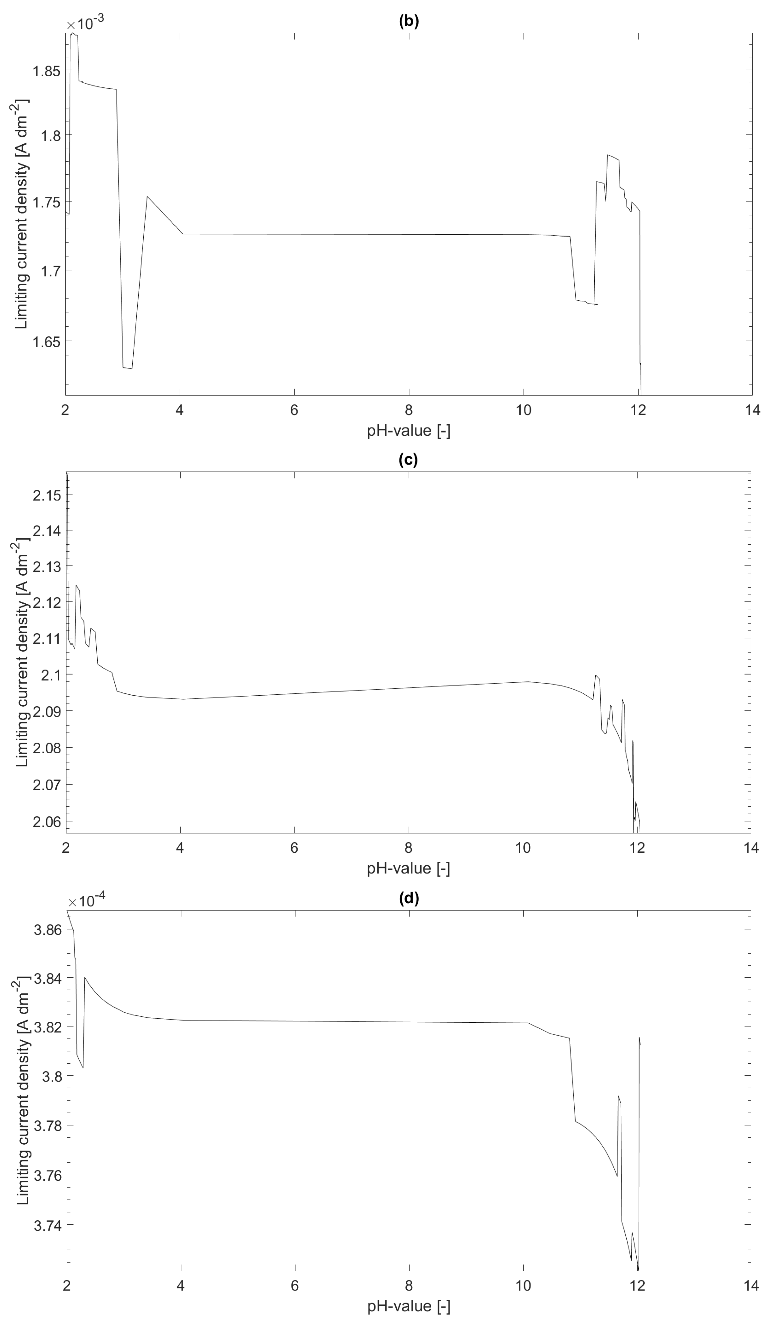
In Figure 1, the limiting current density distributions over the pH value for ${\delta }_X=21\mathsf{\mu }\mathrm{m}$ and $m_{{\mathrm{CO}}_3}=0.5\frac{\mathrm{mol}}{\mathrm{l}}$ (a) and for ${\delta }_X=21\mathsf{\mu }\mathrm{m}$ and $m_{{\mathrm{CO}}_3}=0.75\frac{\mathrm{mol}}{\mathrm{l}}$ (b) are shown. The limiting current density for ${\delta }_X=31\mathsf{\mu }\mathrm{m}$ and $m_{{\mathrm{CO}}_3}=0.5\frac{\mathrm{mol}}{\mathrm{l}}$ (c) and for ${\delta }_X=31\mathsf{\mu }\mathrm{m}$ and $m_{{\mathrm{CO}}_3}=0.75\frac{\mathrm{mol}}{\mathrm{l}}$ (d) are shown as well. As it can be seen in the figure, the current-density distributions for $m_{{\mathrm{CO}}_3}=0.75\frac{\mathrm{mol}}{\mathrm{l}}$ are lower than for $m_{{\mathrm{CO}}_3}=0.5\frac{\mathrm{mol}}{\mathrm{l}}$. This can be expected, since the more ${\mathrm{CO}}_3$ is in the system the higher is the mass of metal ions bound to the $\mathrm{Cu}{\mathrm{CO}}_3$ complex and, hence, the free metal concentration $c_{\mathrm{Cu}}$ is lower. A second observation is that the current–density distribution is strongly dependent on the assumed thickness ${\delta }_X$ of the diffusion boundary layer. The last observation is that the limiting current density seems to decrease as the pH value increases. This observation corresponds with the expectations since the free metal concentration in thermodynamic equilibrium decreases as the pH value increases.

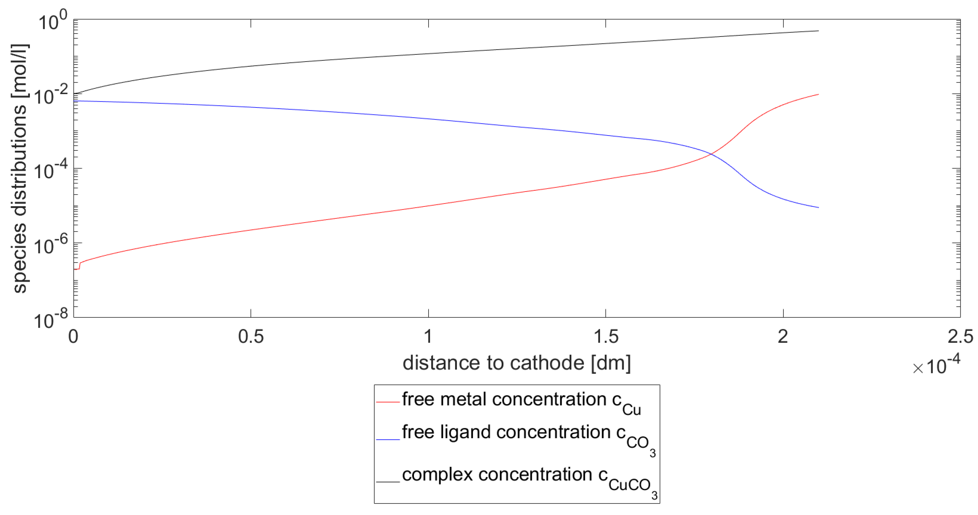
In Figure 2, the species concentrations for the Cu species, ${\mathrm{CO}}_3$ species and the ${\mathrm{CuCO}}_3$ species for $m_{{\mathrm{CO}}_3}=0.5\frac{\mathrm{mol}}{\mathrm{l}}$ and ${\delta }_X=21\mathsf{\mu }\mathrm{m}$ at a pH value of 2 are shown. As can be seen in the figure, the Cu concentration decreases with the distance to the cathode. The same behavior can be seen for the complex concentration $c_{{\mathrm{CuCO}}_3}$. This behavior can immediately be explained by the reaction kinetics, i.e., the mass of free Cu ions decreases by the deposition at the cathode. This effects the mass of free Cu ions that can be bound in the complex as well. As a consequence, the ligand concentration increases as the distance to the cathode decreases.

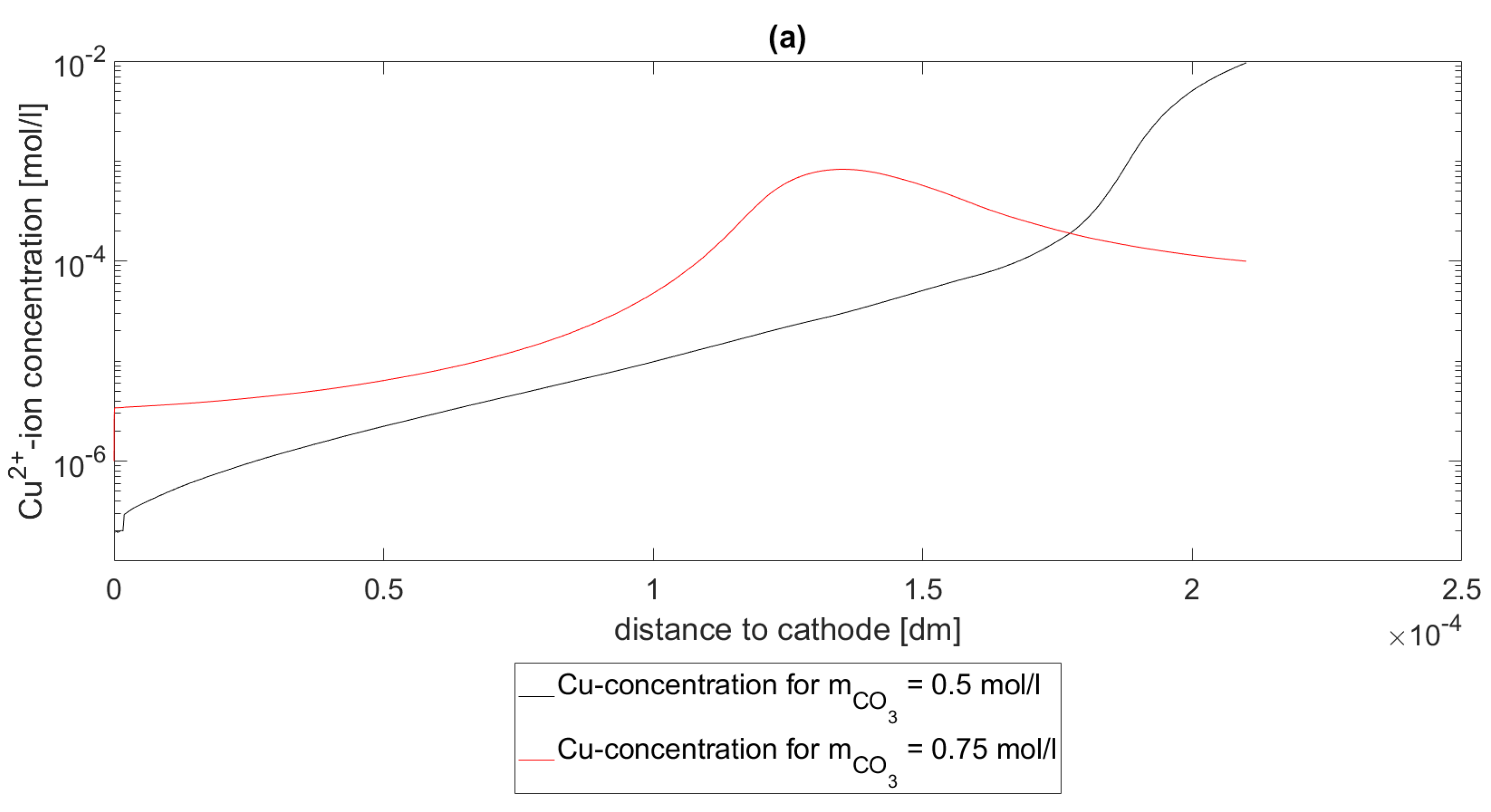
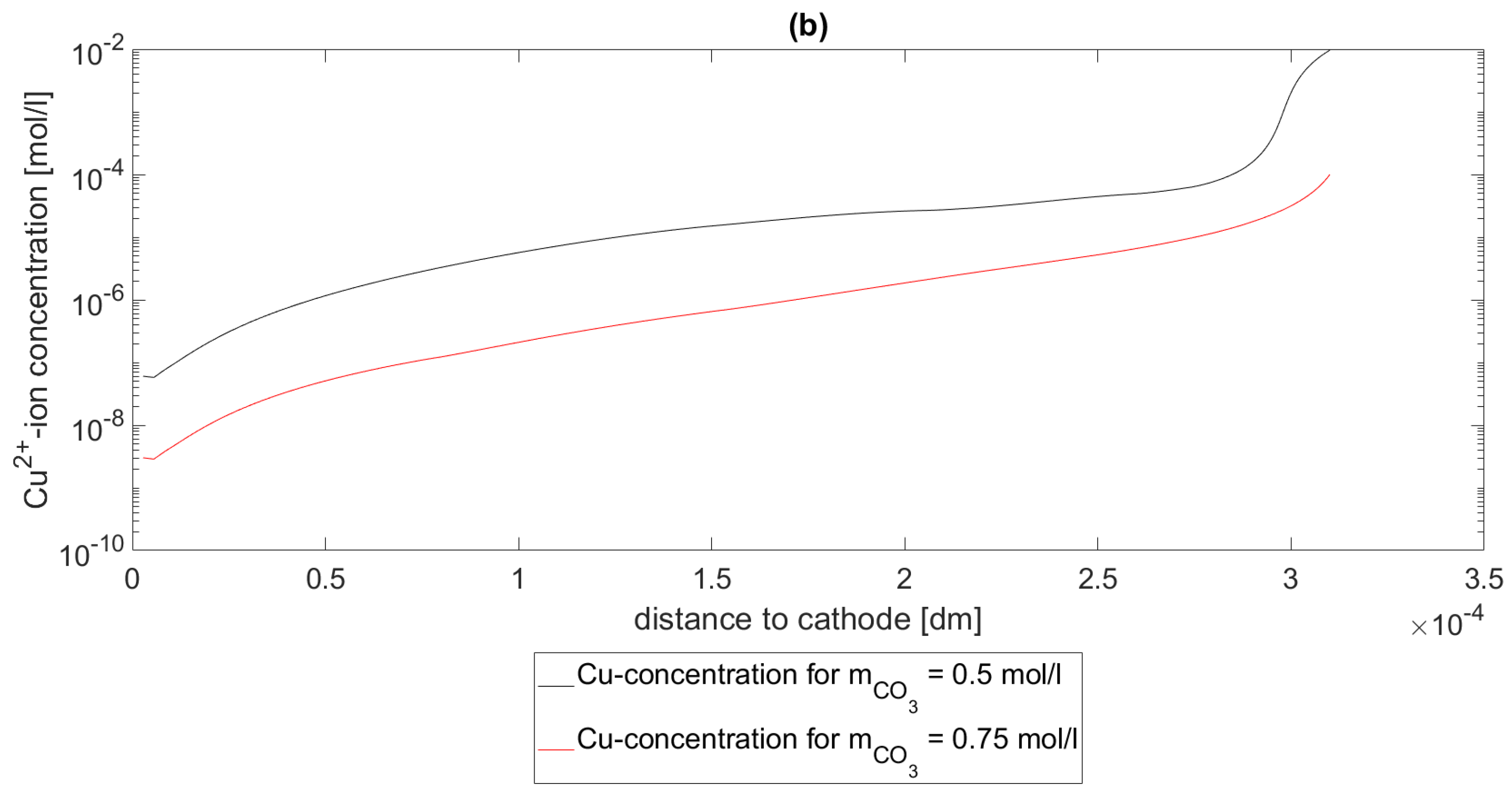
In Figure 3, the Cu concentrations $c_{\mathrm{Cu}}$ are depicted at a pH value of 2. In subfigure (a), the concentration profiles $c_{\mathrm{Cu}}$ of the Cu species for $m_{{\mathrm{CO}}_3}=0.5\frac{\mathrm{mol}}{\mathrm{l}}$, $0.75\frac{\mathrm{mol}}{\mathrm{l}}$ and ${\delta }_X=21\mathsf{\mu }\mathrm{m}$ are shown. In subfigure (b), the concentration profiles $c_{\mathrm{Cu}}$ of the Cu-specie for $m_{{\mathrm{CO}}_3}=0.5\frac{\mathrm{mol}}{\mathrm{l}}$, $0.75\frac{\mathrm{mol}}{\mathrm{l}}$ and ${\delta }_X=31\mathsf{\mu }\mathrm{m}$ are shown. As seen in both subfigures, the concentrations decrease as $m_{{\mathrm{CO}}_3}$ increases. In this setting, this means that the more ${\mathrm{CO}}_3$ is in the system the more Cu is bound in the complex $\mathrm{Cu}{\mathrm{CO}}_3$, which makes this result expected.

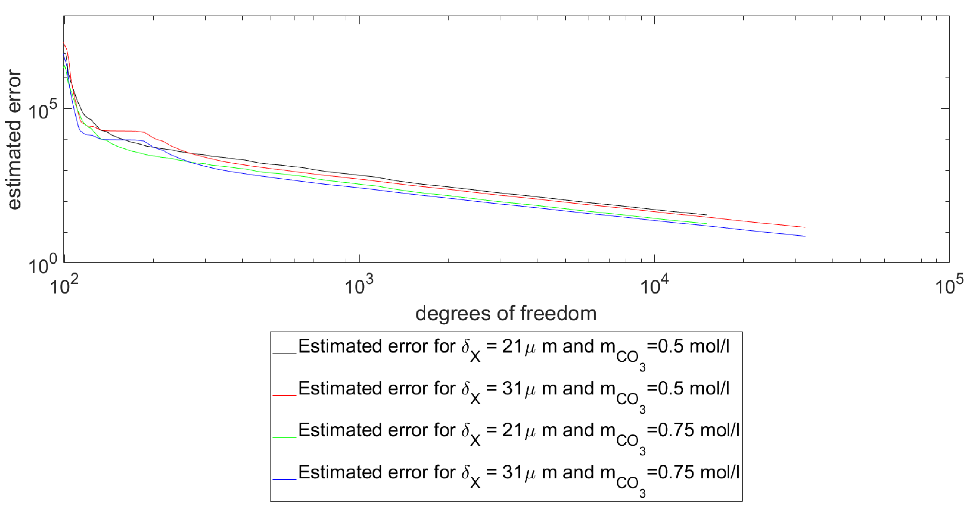
In Figure 4, the estimated error of the approximate solutions $x_h$ are shown. In this context, the error was estimated by the evaluation of the least-squares functional $LS\left(x_h\right)$. As it can be seen in Figure 4, the evaluation of the error estimator experimental setups and pH values. As can be seen directly, the simulations used for the experimental evaluations are in the convergent part of the graphs and have, in comparison to the initial errors, sufficient low evaluations of the error estimator such that the simulations can be considered reliable.

In

Table 2. List of computed limiting current densities (LCD) on the basis of the model described in [13] and the manuscript described in Section 2.

pH-Value	${\mathit{m}}_{{\mathbf{CO}}_3}$	${\mathit{\delta }}_{\mathit{X}}$	LCD from the Literature Model	LCD from the New Model
	$\frac{\mathbf{mol}}{\mathbf{l}}$	$\mathsf{\mu }\mathbf{m}$	$\frac{\mathbf{A}}{{\mathbf{dm}}^2}$	$\frac{\mathbf{A}}{{\mathbf{dm}}^2}$
2	21	0.5	655.1869 × 10${}^{-6}$	296.8710 × 10${}^{-3}$
2	31	0.5	443.8363 × 10${}^{-6}$	1.7425 × 10${}^{-3}$
2	21	0.75	62.9720 × 10${}^{-3}$	2.1565
2	31	0.75	42.6585 × 10${}^{-3}$	386.7841 × 10${}^{-6}$
4	21	0.5	648.7977 × 10${}^{-6}$	330.0978 × 10${}^{-3}$
4	31	0.5	439.5081 × 10${}^{-6}$	1.7261 × 10${}^{-3}$
4	21	0.75	62.3550 × 10${}^{-3}$	2.0931
4	31	0.75	42.2404 × 10${}^{-3}$	382.2545 × 10${}^{-6}$
10	21	0.5	648.6060 × 10${}^{-6}$	330.0053 × 10${}^{-3}$
10	21	0.5	439.3783 × 10${}^{-6}$	1.7257 × 10${}^{-3}$
10	21	0.75	62.3364 × 10${}^{-3}$	2.0979
10	31	0.75	42.2279 × 10${}^{-3}$	382.1442 × 10${}^{-6}$
12	21	0.5	637.8666 × 10${}^{-6}$	295.7975 × 10${}^{-3}$
12	31	0.5	432.1032 × 10${}^{-6}$	1.7447 × 10${}^{-3}$
12	21	0.75	61.2992 × 10${}^{-3}$	2.0636
12	31	0.75	41.5253 × 10${}^{-3}$	372.5681 × 10${}^{-6}$

a comparison of evaluations of the limiting current density (LCD) w.r.t. the model described in [13] and derived in this paper is undertaken. The evaluations vary over pH values, the discussed mass differences of ${\mathrm{CO}}_3$$m_{{\mathrm{CO}}_3}=0.5\frac{\mathrm{mol}}{\mathrm{l}}$ and $m_{{\mathrm{CO}}_3}=0.75\frac{\mathrm{mol}}{\mathrm{l}}$ and the thickness ${\delta }_X$ of the Nernst diffusion layer ${\delta }_X=21\mathsf{\mu }\mathrm{m}$ and ${\delta }_X=31\mathsf{\mu }\mathrm{m}$. As seen in the table the following observations can be made. Both models predict, in each case, a decrease of the limiting current density as the pH value increases. Furthermore it can be seen that, in both models, the limiting current densities for ${\delta }_X=21\mathsf{\mu }\mathrm{m}$ tend to be higher than for ${\delta }_X=31\mathsf{\mu }\mathrm{m}$. Additionally it can be seen that, as expected, the limiting current density is in both models higher, when considering higher ligand masses.

Comparing the values for the new model and the model described in [13] in Table 2, one sees that the computed values of the LCD from the new model are a factor of ${10}^3$ higher than the LCD from the old model. Exceptions from this rule are the values for ${\delta }_X=31\mathsf{\mu }\mathrm{m}$ and $m_{{\mathrm{CO}}_3}=0.75\frac{\mathrm{mol}}{\mathrm{l}}$, where the limiting current density from the old model is at the factor ${10}^3$ over the new model. To explain this asymmetric behavior, note that the formula for the LCD in the old model (see [13] and (11)) is derived from an exact and linear solution to the second Fickian law representing the species distribution $c_M$, which implies a linear dependency of the LCD of $\frac{1}{{\delta }_X}$ and $c_{M,\mathrm{eq}}$. In contrast to that the species distribution, $c_M$ is highly nonlinear and, thus, the distribution of the limiting current density over the pH value can be expected to be nonlinear. This can and will explain the asymmetry addressed.

While both models are dependent on the pH value, the total mass of the ligand $m_{{\mathrm{CO}}_3}$ and the thickness of the boundary layer ${\delta }_X$, the variance of the values with the new model seems to be higher and to underly a more complex nonlinear law than described in [13]. Additionally, it can be seen that, in most cases, the predicted limiting current density from the new model is higher than the respective value from the model described in [13].

In total, the new model behaves as expected. Although a strong dependency of the limiting current density of the thickness ${\delta }_X$ of the diffusion boundary layer is shown, the experiments also show that the model can be used to study the pH dependencies of the limiting current density of an electrolyte and the recipe of the electrolyte can be studied as well. Furthermore, the model can be applied to determine possible alternatives for toxic ligands.

4. Discussion and Conclusions

In this paper, namely in Section 2, an abstract model for the limiting current density was derived. The model described in Section 2 assumes thermodynamic equilibrium of a broad system of reactions in the bath (1), described by the Equations (2a)–(2e). Additionally, it is assumed that, in the diffusion boundary layer at the cathode, only one reaction, namely (3), takes place. Additionally it is assumed that the species concentrations w.r.t. the metal M, the ligand L and the complex K obey the diffusion in the boundary layer. The corresponding physical behavior was described by a stationary system of diffusion and reaction–diffusion equations. Through a convenient definition of the boundary conditions and a reformulation of the arising problem into an obstacle problem to treat possible negative species concentrations, it was possible to compute the limiting current density $j_{\lim }$ from the metal concentration $c_M$ through (8).

In Section 3, an electrolyte was numerically studied. As a result of the numerical experiments, it can be seen directly that the limiting current density is strongly dependent on the mass input $m_L$ and $m_M$ as well as the assumed thickness ${\delta }_X$ of the corresponding boundary layer.

Although the model formulation for the limiting current density is relatively simple, especially only using the language of ODEs (ordinary differential equations), it is strongly biased. For instance, the system of reactions in the bath, which is assumed to be in thermodynamic equilibrium, may and will be much larger than the single reaction assumed to take place in the diffusion boundary layer, but can be expected to be more precise than the model described in [13], since first the thermodynamic equilibrium at the boundary of the Nernst diffusion layer is introduced and a reaction is introduced in the layer domain; hence, missing reactions are respected.

As discussed in Section 3, the computed value of the limiting current density strongly depends on the assumed thickness of the diffusion boundary layer ${\delta }_X$. Similar results, concerning the dependency on ${\delta }_X$, are presented in [8]. Besides the formula given in Remark 1 there are approaches to computing the thickness, as in [10], relying on the currents in the layer but having its own biases. A convenient way to determine the thickness of the diffusion layer would be a direct measurement of the boundary layer. A method to measure it is described in [21], which relies on the measurement of the changes in pH value under the change in time. Further measurements for laminar and turbulent flows of electrolyte are described in [22].

Another bias, which it is necessary to discuss, is the assumption of the thermodynamic equilibrium in the bath. As discussed in [1,4,5,23], the transport processes in the bulk electrolyte are dominated by diffusion, migration, convection and reactions. Assuming, as in [7,8,11,12], that the concentration gradients are low, a concentration gradient will normally exist and, hence, thermodynamic equilibrium will not be fulfilled. Additionally, as it is commonly known, see [24,25,26], the transport processes are strongly geometry-dependent and hence, gradients of the species distributions are also geometry-dependent. In particular, it is typically assumed that the diffusion boundary layer lies within a laminar boundary layer, the thickness of which will differ along the corresponding cathode surface, which will bound the thickness of the diffusion boundary layer due to the geometry dependence of the mechanical flow of the electrolyte (see [26]).

Beyond the biases discussed above, the model has various advantages. For instance the model is relatively easy, and it can be evaluated with a relatively small numerical cost. Even though deviations between the experiment and the model prediction are expected, the model can be used for a more general, qualitative comparison. For example, as discussed in Section 3, electrolytes can be studied within a variation of the pH value. Additionally, the software can be used to compare electrolyte mixtures wherein the ratio of $m_L$ to $m_M$ is varied. Additionally, the model can be used to determine possible substitutes for toxic ligands. The last point is of considerable importance in designing, for example, REACH-compliant electrolytes. In those cases, the model will be sufficient.

In summary, a model was introduced, which, on the one hand, is highly biased, and has, on the other great value in the comparative development of electrolytes. For the formulation of a quantitative, more precise model, more research is needed. The simplest approach to defining such a model is to extend the model to a geometrically and specifically known setup, such as the description of the complete cell, only considering the distance from anode and cathode as the important geometrical feature. This geometrical adjustment needs the inclusion of migration and further reactions assumed to be not in thermodynamic equilibrium.